| Issue |
A&A
Volume 591, July 2016
|
|
|---|---|---|
| Article Number | A61 | |
| Number of page(s) | 11 | |
| Section | Extragalactic astronomy | |
| DOI | https://doi.org/10.1051/0004-6361/201527448 | |
| Published online | 13 June 2016 | |
Dominance of outflowing electric currents on decaparsec to kiloparsec scales in extragalactic jets
1 Dept. of Mathematical Sciences, University of Massachusetts Lowell, Lowell 01854, USA
e-mail: This email address is being protected from spambots. You need JavaScript enabled to view it.
2 Dept. of Physics, University College Cork, Cork, Ireland
3 Research Center for Astronomy and Applied Mathematics, Academy of Athens, 11527 Athens, Greece
4 National Research Nuclear University, 31 Kashirskoe highway, 115409 Moscow, Russia
5 NASA/GSFC, Code 663, Greenbelt, MD 20771, USA
6 Dublin Institute for Advanced Studies, Astronomy and Astrophysics Section, 31 Fitzwilliam Place, Dublin 2, Ireland
Received: 25 September 2015
Accepted: 31 March 2016
Abstract
Context. Helical magnetic fields embedded in the jets of active galactic nuclei (AGNs) are required by the broad range of theoretical models that advocate for electromagnetic launching of the jets. In most models, the direction of the magnetic field is random, but if the axial field is generated by a Cosmic Battery generated by current in the direction of rotation in the accretion disk, there is a correlation between the directions of the spin of the AGN accretion disk and of the axial field, which leads to a specific direction for the axial electric current, azimuthal magnetic field, and the resulting observed transverse Faraday–rotation (FR) gradient across the jet, due to the systematic change in the line-of-sight magnetic field.
Aims. We consider new observational evidence for the presence of a nested helical magnetic-field structure such as would be brought about by the operation of the Cosmic Battery, and make predictions about the expected behavior of transverse FR gradients observed on decaparsec and kiloparsec scales.
Methods. We have jointly considered 27 detections of transverse FR gradients on parsec scales, four reports of reversals in the directions of observed transverse FR gradients observed on parsec–decaparsec scales, and five detections of transverse FR gradients on decaparsec–kiloparsec scales, one reported here for the first time. We also consider seven tentative additional examples of transverse FR gradients on kiloparsec scales, based on an initial visual inspection of published Very Large Array FR maps of 85 extragalactic radio sources, for three of which we have carried out quantitative analyses in order to quantitatively estimate the significances of the gradients.
Results. The data considered indicate a predominance of transverse FR gradients in the clockwise direction on the sky (i.e., net axial current flowing inward in the jet) on parsec scales and in the counter-clockwise direction on the sky (i.e., net axial current flowing outward) on scales greater than about 10 pc, consistent with the expectations for the Cosmic Battery. The predominance of counter-clockwise FR gradients on larger scales has been established at the 3σ confidence level.
Conclusions. The collected results provide evidence for a reversal in the direction of the net azimuthal magnetic field determining the ordered component of the observed FR images, with distance from the jet base. This can be understood if the dominant azimuthal field on parsec scales corresponds to an axial electric current flowing inward along the jet, whereas the (weaker) dominant azimuthal field on kiloparsec scales corresponds to a outward-flowing current in the outer sheath of the jet and/or an extended disk wind. This is precisely the current/magnetic field structure that should be generated by the Cosmic Battery.
Key words: accretion, accretion disks / galaxies: active / galaxies: jets / galaxies: magnetic fields / magnetic fields
© ESO, 2016
1. Introduction
1.1. Faraday rotation in radio sources
There are two ways of probing the geometry of magnetic fields in astrophysical plasmas: (i) the intrinsic orientation of the polarization angle of synchrotron radiation provides information about the projection of the synchotron magnetic field onto the plane of the sky and (ii) Faraday rotation (FR) – the wavelength-dependent rotation of the intrinsic polarization angle of linearly polarized radiation as it traverses a magnetized plasma – provides information about the line-of-sight component of the magnetic field in the region of Faraday rotation. Because Faraday rotation provides information only about the line-of-sight magnetic field, the full three-dimensional (3D) structure of the field cannot be deciphered uniquely solely from direct or synthesized FR observations. This drawback can, in principle, be overcome by modeling the polarized emission regions and the embedded magnetic field and projecting model Faraday rotation-measure (RM) maps onto the observer’s sky to enable direct comparisons (Murgia et al. 2004; Laing et al. 2006; 2008; Guidetti et al. 2010; Govoni et al. 2010; Bonafede et al. 2010). Model RM maps constructed in this way use a minimal set of assumptions to avoid imposing preconceived notions about the plasma and the magnetic field and their interactions with the surrounding intergalactic environment. This type of modeling for galaxy clusters implies mean inter-cluster magnetic-field strengths of a few to several tens of μG and the presence of a random component on scales of ~1 kpc in radio galaxies that are members of large clusters and small groups (Laing et al. 2006; 2008; Guidetti et al. 2010; Bonafede et al. 2010).
The polarization structure observed in the jets of extragalactic radio sources can be used to construct models for the structure of the underlying magnetic field in the jets. Such models of the magnetic field and the FR of the radiation emitted by the jets and the lobes of extragalactic radio sources have been broadened in scope by including physical assumptions about the 3D structure of the field, the kinematics and emissivity of the jet outflow, and the presence of cavities around the jets (Laing et al. 2006; 2008).
1.2. Magnetic fields in jets
It is now well understood that an active galactic nucleus (AGN) consists of two components: a rotating supermassive (~ 108 M⊙) black hole with its event horizon extending out to ~1 AU, and a surrounding rotating accretion disk extending out to ~1 pc. It is widely believed that the physical mechanism that drives these systems is magnetohydrodynamical: the rotating accretion disk is threaded by a magnetic field that is wound up by the differential rotation of the disk plasma (i.e., the field becomes helical), driving a collimated outflow (jet) above and below the symmetry plane of the disk. The asymptotic velocity attained by the jet material is of the same order as the rotational velocity at the base of the jet. The jets are also expected to include two components: an inner, relativistic, axial jet and an outer, nonrelativistic, extended disk wind (Pelletier et al. 1988; Ferreira et al. 2006). The theoretical details of the jet launching mechanism have been well-studied in the literature (Blandford & Payne 1982; Contopoulos & Lovelace 1994; Contopoulos 1995; see also the review by Spruit 2010, and references therein). It is expected that the magnetic field is efficiently wound up only beyond the Alfvén distance, which is ~10 times the radial extent of the outflow at its base. Thus, these theoretical models suggest that the magnetic fields of the inner jet and the outer extended wind will develop significant toroidal components on distances beyond ~10 AU and ~10 pc, respectively, from the base of the jet (see Fig. 1).
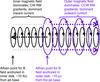 |
Fig. 1 Schematic of the key transition points along the jet axis (not to scale): the Alfven point for the inner field, which lies roughly 10 AU from the jet base, and the Alfven point for the outer field, which lies roughly 10 pc from the jet base. The jet base is located further to the left. Ellipses representing the azimuthal component of the inner field are shown in black, and ellipses representing the azimuthal component of the outer field in blue. In each case, the orientation of the field is shown by corresponding arrows. The associated currents are shown by the dashed lines. CW RM gradients and inward currents dominate on parsec scales, while CCW RM gradients and outward currents dominate on decaparsec–kiloparsec scales. |
The old idea that loops of weak field can be generated randomly by the Biermann (1950) battery in the accretion disks, where they are amplified by turbulent dynamos, so that their tangled fields are embedded in the outflows, has not been successful in explaining the observations. Recent radio observations indicate the presence of magnetic fields organized on scales of at least ~10–30 kpc in AGN (e.g., Carilli & Taylor 2002; Widrow 2002; Eilek 2003; Kronberg 2005; 2010). Furthermore, the inefficacy of this mechanism has been recognized in various theoretical studies (e.g., Vainshtein & Rosner 1991; Subramanian 2008; Kulsrud & Zweibel 2008). Despite these problems, the Biermann battery continues to be adopted as the physical basis in investigations of magnetic-field generation in AGN, because of the perceived lack of an alternative mechanism.
1.3. The Cosmic Battery
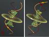 |
Fig. 2 Schematic of the helical-field structure of an AGN for arbitrary observer orientation as predicted by the Cosmic Battery. The central black hole is represented by the gray sphere, the surrounding accretion disk by the flattened yellow disk, and the axis of the system by the gray line. The white arrow indicates the direction of the disk/black hole rotation. Inner field lines threading the black hole are yellow and green. Outer field lines threading the disk are orange and red. The Cosmic Battery predicts that the axial direction of the inner/outer field is along/opposite to ω, respectively (Eq. (1)). This corresponds to an axial electric current flowing inward along the jet axis and outward farther out where the outer field lines are drawn. Field lines are wound by the black hole/disk rotation. An observer will see the transverse RMs increasing on the sky CW/CCW relative to the jet base for the inner/outer azimuthal field. |
In the past few years, a promising alternative to the Biermann battery has been found, which seems capable of generating strong, ordered, large-scale magnetic fields in AGN accretion disks and of providing the physical background needed to understand some of the most prominent features observed in magnetized jets. This alternative mechanism relies on the Poynting-Robertson drag on plasma electrons to generate large-scale azimuthal currents in the inner disks of AGN (Contopoulos & Kazanas 1998; Contopoulos et al. 2006; 2015; Christodoulou et al. 2008; Lynden-Bell 2013; Koutsantoniou & Contopoulos 2014). Its most important element is that it supports and maintains a large-scale poloidal magnetic field whose direction is inextricably tied to the rotation of the disk (see also Lynden-Bell 2013). In the vicinity of a 108 M⊙ black hole, this mechanism can generate a field corresponding to equipartition between the magnetic and relativistic-particle energies on timescales of the order of one billion years (Contopoulos & Kazanas 1998; Contopoulos et al. 2015). We call this mechanism the Cosmic Battery (hereafter CB).
According to the CB, the Poynting-Robertson drag force on the electrons at the inner edge of the accretion disk around an AGN’s supermassive black hole1 generates a toroidal electric current which gives rise to poloidal magnetic field loops around the inner edge of the disk with a magnetic moment μB. The outer footpoint of each loop resides well inside the accretion disk and diffuses outward on the disk’s local diffusion timescale, provided that this is at least about a factor of two shorter than the local accretion timescale. The inner footpoint is dragged inward by the accretion flow and eventually ends up near the black hole. Under these conditions, the magnetic flux that accumulates in the vicinity of the black hole due to the continuous (secular) growth of the inner field always points in the same direction as the angular velocity vector ω of the accretion disk:  (1)The footpoints of each poloidal loop also participate in the rotation of the disk, thus they are both dragged along the direction of rotation. The resulting wound-up field configuration corresponds to a large-scale axial electric current ℐinner that flows toward the disk along the symmetry axis of the inner (core) jet, i.e.,
  (2)and a large-scale axial electric current ℐouter that outflows from the disk and into the outer wind, i.e.,
  (3)(see Fig. 1). The central jet current closes along the interface between the core jet and the outer wind, whereas the outer wind electric current closes farther out (not along the inner core jet). This universal configuration of the axial electric current circuit in extragalactic jets, predicted by Contopoulos et al. (2009, hereafter CCKG), is unique to the CB mechanism and it was confirmed numerically by the simulations of Christodoulou et al. (2008) and Contopoulos et al. (2015).
1.4. Observational signatures of the Cosmic Battery
The most obvious diagnostic tool of the above magnetic-field configuration is the observation of characteristically oriented transverse Faraday RM gradients across the jets and the lobes of at least some radio sources that are not too disturbed by interactions with their environment or other internal factors. As depicted in Figs. 1 and 2, when the observed RMs increase in the clockwise (CW) direction on the sky relative to the base of the jet outflow, the electric current flows inward opposite to the jet direction, whereas if the RMs increase in the counterclockwise (CCW) direction on the sky relative to the jet base, the electric current flows outward along the jet direction. In summary:  These results are independent of observer location (see Fig. 2 and CCKG for more details). Now, as was pointed out above (see Fig. 1), the inner field should be efficiently wound up only outside the corresponding Alfvén point, meaning at distances greater than about 10 AU from the jet base; in terms of observed transverse Faraday RM gradients due to the systematic change in the line-of-sight component of the azimuthal field, we expect the inner azimuthal field and ℐinner to give rise to significant transverse Faraday RM gradients only at distances greater than about 10 AU from the jet base. Analogously, the outer field should be efficiently wound up only at distances greater than about 10 pc from the jet base; accordingly, we expect the outer azimuthal field and ℐouter to begin making significant contributions to the Faraday RM gradients only at distances greater than about 10 pc from the jet base. This suggests that the net Faraday rotation due to both the inner and outer azimuthal fields (i.e., the net transverse RM gradient), should be dominated by the inner azimuthal field at distances out to about 10 pc from the jet base, then by the outer azimuthal field starting at distances of about 10 pc or more (see Fig. 1). There could also be a region at distances of a few tens of pc where no clear transverse RM gradients are observed, because the contributions from the inner and outer azimuthal fields are comparable.
CCKG looked for precisely this effect using published RM maps for roughly 30 AGNs whose parsec-scale jets mapped with very long baseline interferometry (VLBI) seemed to show reasonably clear transverse RM gradients. CCKG reported evidence for a predominance of CW transverse RM gradients within ≃ 20 pc of the center, whereas CCW transverse RM gradients were found in some of these sources at larger distances. These results were disputed by Taylor & Zavala (2010), who claimed that, in the vast majority of cases, the VLBI jets were too poorly resolved to make the observed transverse RM gradients reliable. However, the Monte Carlo simulations of Hovatta et al. (2012) and Mahmud et al. (2013) subsequently demonstrated that transverse RM gradients could be detected even when the intrinsic jet width was much narrower than the beam width for the VLBI array used, removing the doubts cast by Taylor & Zavala (2010). Previously firm results, recently reported new results and reanalyses of a number of previously published RM images applying the improved error estimation approach developed by Hovatta et al. (2012) have now brought the list of reliable (monotonic, with significances > 3σ) parsec-scale transverse RM gradients to 27, of which 20 are CW and 7 are CCW on the sky, relative to their jet bases (Gomez et al. 2008; Kharb et al. 2009; Hovatta et al. 2012; Gabuzda et al. 2014a,b, 2015a); a simple binomial probability distribution analysis indicates that the probability of at least 20 out of 27 of the observed transverse RM gradients having the same orientation (CW) by chance is about 0.95%, supporting the reports of CCKG of a predominance of CW transverse RM gradients on parsec scales. In the sizeable minority of parsec-scale jets displaying CCW transverse RM gradients (7 out of 27), the gradients may be present at distances from the cores that are greater than the transition distance of about 20 pc; a more detailed analysis of this question will be considered by Gabuzda et al. (in prep.). In addition, it is always possible that the battery mechanism is not efficient in some jet-disk systems. Work is ongoing to try to add to the list of AGN jets with reliable transverse RM gradients on parsec scales (Gabuzda et al., in prep.). A precise demarkation line between the distances at which the inner and outer azimuthal magnetic fields dominate the observed transverse RM gradients cannot be determined with certainty from the available VLBI data, but the outer (return) field with its CCW RM gradients appears to dominate at distances larger than about 20 pc (Fig. 2 in CCKG), at least in those objects in which the RM gradients are resolved and are not obscured by substantial random RM components.
1.5. Outline of the paper
With the above theoretical considerations in mind, we set out to examine the available information about transverse RM gradients on larger scales extending out to kiloparsecs, exceeding the expected distance of the Alfvén point for the outer azimuthal magnetic field from the jet base. The purpose of this study is essentially twofold: (i) to establish whether or not transverse RM gradients reasonably interpreted as reflecting the presence of helical jet magnetic fields are present on scales of tens to thousands of parsec and, if present; (ii) to establish whether such RM gradients show any evidence for a preferred direction.
In Sect. 2, we describe observations for three sources we have analyzed for this paper. In Sect. 3, we consider three previous firm reports of transverse RM gradients on scales exceeding about 20 parsec, for which quantative analyses have already been carried out in previous publications, to which we add our new detection of a 3.0σ transverse RM gradient in A2142A. We also consider four reliable cases of reversals in the direction of the observed RM gradients with distance from the jet base. Finally, we consider an additional seven transverse RM gradients that are visible in previously published RM maps, and present the results of quantitative analyses of the RM results for three of these sources. All seven of these transverse RM gradients must be considered tentative, due to insufficiently high significance of the gradients (< 3σ), lack of information about the uncertainties in the observed RM values, and/or uncertainty in the orientation of the gradients relative to the local jet direction. In Sect. 4, we discuss the implications of these collected results both in general and in the context of the CB mechanism. Finally, we conclude in Sect. 5 with a summary of our results and some remarks about related ongoing research of the large-scale magnetic fields in AGNs and in our own Galaxy.
2. Observations and reduction
2.1. VLA data
A. Bonafede and F. Govoni kindly provided the calibrated visibility data that had been used to make the published RM maps for A2142A (Govoni et al. 2010) and 5C4.152 (Bonafede et al. 2010). Data are available for 5C4.152 at 4.635, 4.835 and 8.275 GHz, and for A2142A at 4.535, 4.835, 8.085, and 8.465 GHz. The observations and data calibration and reduction methods used in the initial analyses carried out for these objects are given by Bonafede et al. (2010) and Govoni et al. (2010).
We could not use the RM maps published by Bonafede et al. (2010) and Govoni et al. (2010) directly, because the associated error maps did not take into account the finding of Hovatta et al. (2012) that the uncertainties in the Stokes Q and U fluxes in individual pixels on-source are somewhat higher than the off-source rms fluctuations, potentially increasing the resulting RM uncertainties.
To address this, we imported the final, fully self-calibrated visibility data into theAIPS package, then used these data to make naturally weighted I, Q and U maps at all wavelengths, with matching image sizes, cell sizes and beam parameters specified by hand in theAIPS taskIMAGR. These images were all convolved with a circular Gaussian beam having a full-width at half-maximum of 3′′. We obtained maps of the polarization angle,  , and used these to construct corresponding RM maps in theAIPS and CASA packages. The uncertainties in the polarization angles used to obtain the RM fits were calculated from the uncertainties in Q and U, which were estimated using the approach of Hovatta et al. (2012). In all cases, satisfactory RM fits were obtained without applying nπ rotations of the observed polarization angles.
2.2. VLBA data
We also analyzed the RM distribution of 3C 120, constructed using data obtained with the Very Long Baseline Array (VLBA) at 1.358, 1.430, 1.493 and 1.665 GHz. This RM map was originally published by Coughlan et al. (2010); again, we were not able to use the previously published RM map directly because the associated error maps did not take into account the improved method of Hovatta et al. (2012) for estimating the on-source Q and U uncertainties in individual pixels.
We addressed this by using the Q and U maps used by Coughlan et al. (2010) to produce new RM maps in bothAIPS andCASA, assigning Q and U uncertainties in accordance with the approach of Hovatta et al. (2012).
In all cases, when differences in RM values across the jet were obtained, the uncertainties of the RM values did not include the effect of uncertainty in the polarization angle calibration, since this cannot introduce spurious RM gradients (Mahmud et al. 2009; Hovatta et al. 2012). The uncertainty of the difference between the RM values at the two ends of a slice was estimated by adding the uncertainties for the two RM values in quadrature.
3. Transverse RM gradients on scales exceeding ≃20 pc
3.1. Previously published firm gradients
Virtually all the work done on transverse RM gradients has been carried out for high-resolution data obtained on the VLBA at wavelengths between 15 and 5 GHz; most of the RM gradients detected cross their jets at projected distances from the jet base of no more than a few milliarcseconds (less than about 20−30 pc). Very few studies probing larger scales have been carried out, and we will now consider the few results available here. In all cases, the statistical significances of the transverse RM gradients have been reliably estimated, and found to be at least 3σ. When we refer to a transverse RM gradient being CW or CCW, we mean that its orientation is clockwise or counter-clockwise on the sky, relative to its own jet base.
-
1.
1652+398 (Mrk 501). The RM map of thisAGN based on VLBA data at frequencies between 1.6 and8.4 GHz published by Croke et al.(2010) shows a very clear transverse RM gradient throughout theextended jet before it turns sharply about 30 mas(about 20 pc projected distance) from the core,oriented CCW. Croke et al. (2010) present a quan-tative analysis of this gradient. Even taking into account the factthat the RM uncertainties indicated by Croke et al.(2010) were not obtained using the improved method of Hovattaet al. (2012), and therefore could be up to abouta factor of two too small, the significance of this gradient is far inexcess of 3σ.
-
2.
3C 380. The RM map of this AGN based on VLBA data at wavelengths between 1.4 and 5.0 GHz published by Gabuzda et al. (2014a) shows a transverse RM gradient oriented CCW; the quantative analysis carried out by Gabuzda et al. (2014a) shows that this gradient has a significance of about 4σ.
-
3.
5C4.114. An arcsecond-scale VLA RM map for the kiloparsec-scale jets of 5C4.114 recently analyzed by Gabuzda et al. (2015b) demonstrates transverse RM gradients across both the northern and southern jets with significances of about 4σ and 3σ, respectively, both oriented CCW.
3.2. New detection of a firm transverse RM gradient in A2142A
The radio source A2142A is located in a cluster, and we therefore expect some contribution to the RM distribution from the magnetized intercluster gas; this should most likely not show any large-scale order, and be predominantly “patchy”. In addition to some patchiness, the RM distribution of A2142A shows a tendency for the RM values along the northern side of the jet to be less negative than those along the southern side (Fig. 13 of Govoni et al. 2010), corresponding to a possible gradient in the RM values across the jet. We note that the core is at the eastern end of the observed radio structure, so that this implied transverse RM gradient is oriented CCW.
Figure 3 presents our 4.535-GHz intensity image of A2142A, with the RM image superposed in color; this essentially reproduces the images in Fig. 13 of Govoni et al. (2010). The output pixels in the RM map were blanked when the RM uncertainty resulting from the χ vs. λ2 fits exceeded 80 rad/m2. Our analysis of the entire RM distribution showed the presence of monotonic RM gradients across the jet in the region surrounded by the gray box. At the redshift of A2142A, z = 0.091, these correspond to projected distances of roughly 10 kpc from the jet base. The points in the lower panel of Fig. 3 correspond to monotonic transverse RM gradients obtained for a series of parallel RM slices across the jet, inside the gray box in the upper panel. As can be seen, comparisons of the RM values at the two ends of the RM slices considered indicate that the transverse RM gradients about 4 arcsec from the start of the boxed region have significances reaching about 3.5σ, with another region of gradients reaching nearly 2σ slightly further out from the core. Thus, we consider this a firm case of a transverse RM gradient on kiloparsec scales.
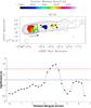 |
Fig. 3 Intensity map at 4.535 GHz of A2142A with the RM distribution superposed (upper panel). The lowest contour is 1% of the peak intensity of 8.8 mJy/beam, the contours increase in increments of a factor of two, and the beam size is shown in the lower left corner of the image. The black arrow across the jet highlights the direction of the transverse RM gradients. The gray box shows the region for which the significances of series of parallel, monotonic transverse RM gradients are plotted in the lower panel; the gray arrow outside the box pointing outward along the jet shows the direction of increasing pixel number in the lower panel, and pixel 0 corresponds to the inner edge of the gray box. Pixel size is 0.25 arcsec. The 2σ level is shown by the dashed blue horizontal line, and the 3σ level by the dashed red horizontal line. |
3.3. Previously published firm RM-gradient reversals
To the four sources in Sects. 3.1 and 3.2, we add information from reports of reversals in the directions of the observed transverse RM gradients in four more AGNs: 0716+714 (Mahmud et al. 2013, reversal at a projected distance of a few pc from the jet base), 0923+392 (Gabuzda et al. 2014b, reversal at a projected distance of about 15 pc from the jet base), 1749+701 (Mahmud et al. 2013, reversal at a projected distance of about 35 pc from the jet base), and 2037+511 (Gabuzda et al. 2014b, reversal about 35 pc from the jet base). Although the observed reversal in the direction of the observed transverse RM gradient in 0716+714 was relatively close to the core, the 1.4−1.7 GHz data analyzed by Healy (2013) show that the orientation of the outer gradient was maintained to projected distances of about 35 pc from the core. In all four cases, quantitative analyses carried out in the papers cited above indicate that both transverse RM gradients detected had significances of at least 3σ, and the inner gradient was oriented CW and the outer gradient CCW relative to the jet base.
3.4. Tentative gradients from an initial inspection of RM maps in the literature
The transverse RM gradients in 5C4.114 and A2142A listed in Sects. 3.1 and 3.2 were initially identified via an initial inspection of published Faraday RM maps of extragalactic radio sources on kiloparsec scales, carried out for 85 objects (Athreya et al. 1998; Best et al. 1998; 1999; Feretti et al. 1999; Venturi & Taylor 1999; Taylor et al. 2001; Eilek & Owen 2002; Goodlet et al. 2004; Govoni et al. 2006; 2010; Laing et al. 2006; 2008; Kharb et al. 2008; Guidetti et al. 2008; 2010; Feain et al. 2009; Kronberg 2009; Bonafede et al. 2010; Kronberg et al. 2011; Algaba et al. 2013). In all cases, the authors of these studies took care to ensure that the RM images were constructed using only data with sufficiently high signal-to-noise ratios, and that the resulting λ2 fits for the RM values were sufficiently good. Unfortunately, full information about the uncertainties in the RM values at individual points in the RM maps is not available; therefore we were able to identify candidate transverse RM gradients, but have not been able to carry out quantitative analyses to test their significances.
We were unable to identify any obvious large-scale monotonic transverse RM gradients in 77 of these 85 published maps, in which (a) the jets appeared to be strongly influenced by their surroundings (they were strongly bent or appeared to be partially disrupted); (b) the RM distribution was patchy; (c) limited to just a few pixels across or along the images (insufficient resolution); (d) the RM images were based on only two frequencies; or (e) the results were shown in gray scale that did not make the structures in the RM images sufficiently clear. We sought to obtain higher-resolution or color images from some authors, and we appreciate their efforts to provide us with the maps we requested.
In the end, we identified eight potential objects whose RM maps showed extended, monotonic, nearly transverse RM gradients. Of these, two (5C4.114 and A2142A) have now been shown to be statistically significant (Gabuzda et al. 2015b; this paper), leaving six additional tentative gradients. To these we add results for 3C 120 on slightly smaller scales of 30–100 pc presented by Coughlan et al. (2010). We have not attempted to measure or analyse the magnitudes of these tentative RM gradients, which would be extremely difficult to interpret unambiguously due to convolution with the observing beam. Instead, we focus on the presence of transverse gradients visible in the RM distributions and their directions relative to the bases of the jets, quantatively estimating the significances of these gradients when possible.
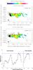 |
Fig. 4 Top panel: intensity map at 1.358 GHz of 3C 120 convolved with the “intrinsic” beam and the RM distribution superposed. The lowest contour is 0.125% of the peak of 1.37 Jy/beam. The middle panel shows the same intensity and RM maps convolved with a circular beam of equal area; the lowest contour is 0.125% of the peak of 1.43 Jy/beam. In both cases, the contour step is a factor of two, the pixel size is 0.25 arcsec, and the beam size is shown in the lower left corner of the image. The bottom panel shows a plot of the significances of a series of transverse RM gradients calculated inside the gray boxes in the middle panel; the 2σ level is shown by the dashed blue horizontal line. See text for more detail. |
We briefly describe the RM distributions of these seven sources, and the basis for our suggestion that these may contain transverse RM gradients. The patchiness of many of the 85 published RM distributions we considered is consistent with a picture in which random distributions of the magnetic field and electron density in the general vicinity of the radio source (e.g., in the cluster or inter-cluster medium in which the source is located) generally dominate on these large scales; these seven sources appear to be those in which an ordered RM pattern is dominant in at least some regions. As above, when we refer to a transverse RM gradient being CW or CCW, we mean that its orientation is clockwise or counter-clockwise on the sky, relative to its own jet base.
-
1.
0156−252. There appears to be an RM gradient across the easternjet (Fig. 3 of Athreyaet al. 1998), oriented in the CCWdirection. Unfortunately, we do not have access to these data andwere not able to quantatively analyze the significance of thisgradient. Therefore, this remains a tentative transverse RMgradient.
-
2.
3C 120. In contrast to the other objects considered in this section, the Faraday-rotation map of Coughlan et al. (2010) is based on VLBA data at four frequencies between 1.4 and 1.7 GHz, and thus probes slightly smaller angular scales. Transverse RM gradients are present at several locations on scales of approximately 30−100 pc from the core, all oriented CCW. The top panel of Fig. 4 presents our 1.358 GHz intensity and RM images of 3C 120 (beam size 19.6 mas × 7.6 mas in position angle 27°); these essentially reproduce the images of Coughlan et al. (2010). The middle panel gives a version of the same RM map convolved with a circular beam (beam radius 12.2 mas). In both cases, the output pixels in the RM maps were blanked when the RM uncertainty resulting from the χ vs. λ2 fits exceeded 20 rad/m2. Both maps show very similar RM structures, and we present our further analysis for the map convolved with the circular beam. Our analysis of the entire RM distribution showed the presence of monotonic RM gradients across the jet in the regions surrounded by the gray boxes. The black arrows in the middle panel highlight the main regions of transverse RM gradients. The points in the bottom panel of Fig. 4 correspond to monotonic transverse RM gradients obtained for a series of parallel RM slices across the jet, inside the gray boxes in the middle panel. The gray arrows pointing outward along the jet in the middle panel show the direction of increasing pixel number in the lower panel: pixel 0 corresponds to the inner edge of the left-hand gray box, and pixel 50 to the inner edge of the right-hand gray box. We can see that these slices reach significances ≃ 2σ at several locations along the jet, but none reach 3σ. Thus, these transverse RM gradients cannot yet be considered firm. However, 3C 120 remains on the list of sources displaying tentative transverse RM gradients; deeper VLBA observations with a wider frequency range could help determine whether these gradients are statistically significant.
-
3.
M 87. Algaba et al. (2013) suggest that there are clear RM gradients across HST-1 and knots A and C. The gradients are all directed CCW. Until a more detailed quantitative analysis is available, this remains a tentative transverse RM gradient.
-
4.
5C4.152. This source has an intriguing RM distribution, with RM gradients present across both lobes (Fig. 15 of Bonafede et al. 2010). The gradient across the southern lobe seems to be fairly orthogonal to the jet direction, while the gradient across the northern lobe appears to be offset from orthogonality as the jet bends toward the east just before the hot spot. If the gradient across the southern lobe can be taken to be transverse to the jet, its direction is CCW. We reconstructed the previously published RM map in order to estimate the significance of these RM gradients. Our quantative analysis of a series of RM slices taken across the southern lobe indicates that the strongest transverse RM gradients have significances of about 1.5σ. This demonstrates that these gradients cannot be considered statistically significant. However, we suggest that it is appropriate to retain 5C4.152 on the list of sources displaying tentative transverse RM gradients, in particular, because the 8-GHz data of Bonafede et al. (2010) had an atypically high noise level, and the uncertainties in the RM values were relatively high as a result of the limited range and number of frequencies used (8.2 GHz, 4.6 GHz, 4.8 GHz). Analysis of kiloparsec-scale observations with lower noise levels and/or a wider frequency range could help determine more conclusively whether these gradients are significant or not.
-
5.
Cen A. After subtracting the overall mean RM (which is presumably foreground), the residual RM map shows a tendency for positive residuals on the eastern side and negative residuals on the western side of the entire northern lobe (Feain et al. 2009). This seems to imply an RM gradient that extends for some 235 kpc across the northern lobe (Fig. 7 of Feain et al. 2009), oriented CCW. The southern lobe is strongly bent and no systematic trends are visible. Although there appears to be a difference in the dominant signs of the residual RM values on either side of the northern jet axis, the RM values themselves do not form a clear gradient across the jet. In addition, RM measurements are available only at the positions of background sources, so that we do not have measurements of a continuous RM distribution across the source. Nevertheless, we were able to test whether the difference in the dominant RM signs was statistically significant by dividing the northern jet/lobe into three sections across the jet, encompassing the declination range from −38° to −41° and the right-ascension ranges 13h15m0s–13h21m59s (western side), 13h22m0s–13h29m59s (central region), and 13h30m0s–13h36m59s (eastern side). We then determined the number of positive and negative RM values in the eastern and western sections; this yielded 15/21 negative RM values in the eastern section and 15/21 positive RM values in the western section. A simple binomial probability analysis indicates that the probability of obtaining 15 or more of 21 values of a particular single sign is 3.92%; if we are interested in the probability of having this fraction of either sign, this must be multiplied by two, and so increases to 7.84%. However, the probability of obtaining 15 or more of 21 values of one sign on one side of the jet, and simultaneously 15 or more of 21 values of the opposite sign on the other side of the jet, is the product of these the two separate probabilities, or (0.0784)(0.0392)(100) = 0.31%, which corresponds to 3σ. Thus, our quantative analysis demonstrates that the asymmetry in the signs of the RM values across the northern jet of Cen A is statistically significant at the 3σ level. However, because it is not possible to test whether this transverse trend in the observed RM values is monotonic and systematic due to the availability of RM measurements only at the positions of background sources, we retain Cen A on the list of sources whose jets display tentative transverse RM gradients.
-
6.
3C 303. Kronberg et al. (2011) report the presence of a transverse RM gradient at the location of knot E3, and use information about this gradient together with certain assumptions to estimate the associated current in the jet. The RM gradient is clearly visible in Fig. 3 of Kronberg et al. (2011), although it is quite narrow and is not well resolved. The direction of the gradient is CCW. Although this RM map has been published in the refereed literature, we include 3C 303 in our list of tentative gradients because the original paper does not provide information about the uncertainties of the single-pixel RM values that can be used to estimate the significance of the RM gradient. We do not have access to these data, and so were not able to carry out our own quantitative analysis for this source.
-
7.
3C 465. The southern jet provides a clear example of a systematic, extended transverse RM gradient that extends along most of this jet (Fig. 6 of Eilek & Owen 2002). The color scale chosen for the RM distribution is such that the RM map presented by Eilek & Owen (2002) is essentially an RM sign map. The orientation of the RM gradient across the southern jet is CCW. The northern jet shows signs that it intrinsically had an overall pattern, but the jet and the RM pattern have become distorted. We do not have access to these data, and so were not able to carry out our own quantitative analysis for this source.
Table 1 summarizes information about all the firm (upper rows) and tentative (lower rows) transverse RM gradients considered in this section. The references in bold in Table 1 indicate the papers in which quantitative analyses are carried out to determine the statistical significances of these gradients. Treating the detections of the transverse RM gradients across the northern and southern jets of 5C4.114 as independent measurements, we have in total nine firm cases of transverse RM gradients. All these transverse RM gradients are oriented CCW relative to their jet bases on comparatively large scales, greater than about 20 pc.
Transverse RM gradients on decaparsec to kiloparsec scales.
4. Discussion
4.1. Transverse RM gradients on scales out to kiloparsecs from the central AGN
The most fundamental implication of the results discussed above is that transverse Faraday rotation gradients – predicted to exist if the jets carry toroidal or helical magnetic fields and detected earlier in some 27 AGNs on parsec scales – are also present on considerably larger scales, extending out to thousands of parsecs (e.g., 5C4.114; Gabuzda et al. 2015b). This is an important result, because if AGN jets carry helical magnetic fields, these should be present on essentially all scales where the jets propagate, provided that the intrinsic field structure of the jet is not disrupted by interactions with the surrounding environment. We note that this conclusion follows from the firm results listed in Sects. 3.1−3.3, and does not depend on the tentative identifications of transverse RM gradients considered in Sect. 3.4.
At the same time, our literature search for transverse RM gradients on kiloparsec scales yielded only eight tentative cases out of 85 objects considered, indicating that it is comparatively difficult to detect transverse RM gradients due to the presence of helical magnetic fields in kiloparsec-scale jets. In fact, it is easy to understand why this should be the case: there is an appreciable turbulent, inhomogeneous component to the thermal ambient media surrounding the jets on these scales, which superposes a more or less random pattern over the systematic pattern due to the helical fields. This random component in the RM distribution apparently dominates in the majority of cases. This makes it perfectly natural that most of the observed RM distributions appear random and patchy, but the overall pattern due to the helical fields sometimes comes through. This suggests that, on average, it may be easier to detect the systematic RM component due to helical jet magnetic fields on parsec scales, where the ordered inner field is more dominant, a result that seems to be borne out from the observations (see also Sect. 4 below).
The tentative transverse RM gradients that we consider in Sect. 3.4 were not, in most cases, noticed or appreciated by the authors of the original papers; this is primarily due to the fact that their main interest was in the magnetic fields of the clusters in which the radio sources are located, rather than in the individual radio sources themselves. Eilek & Owen (2002) did note the striking RM distribution in 3C 465, but they did not consider the possibility that it is associated with an embedded magnetic field because the observed Faraday rotation is external to the main radiation source. Bonafede et al. (2010) similarly suggested that the observed RM distributions are due primarily to Faraday rotating material that is not associated with the radio sources themselves, based in part on the observation that the observed Faraday rotation is external; however, their arguments are based on general considerations and statistical relations, rather than on an individual examination of particular objects. Govoni et al. (2010) essentially assumed that the observed RMs are associated only with the intracluster medium, and used the RM observations to deduce the properties of this medium.
In our interpretation, the large-scale Faraday rotation for the vast majority of extragalactic radio sources is indeed dominated by turbulence and fluctuations in the cluster media; but the eight sources we have identified as displaying evidence for monotonic, extended, transverse RM gradients on scales exceeding about 20 parsec (including 5C4.114; Gabuzda et al. 2014b) essentially represent a handful of objects in which the dominant contribution to the Faraday rotation in some regions is due to material associated with the radio source itself, rather than the patchy cluster media. In these cases, the observed Faraday rotation can still be external (not occurring throughout the radiating volume of the source), but it is nevertheless associated with regions carrying the imprint of a helical magnetic field in the immediate vicinity of each AGN jet. Direct evidence that the observed Faraday rotation is external to the main jet volume is indicated by the fact that the RM fits that were obtained when constructing the RM maps do not show significant deviations from λ2 behavior, within the uncertainties (see, e.g., the plots presented by Bonafede et al. 2010; Croke et al. 2010; Govoni et al. 2010; Mahmud et al. 2013; and Gabuzda et al. 2014a). In some cases, the three-dimensional structure of the emitting regions may not be entirely clear; for example, it may not be obvious whether the observed regions of the Faraday-rotation gradients are associated with the outflowing jet or a possibly back-flowing lobe structure. However, in either case, these regions could carry the imprint of the helical magnetic field carried by the jet, so that this uncertainty does not affect the basic interpretation of the Faraday-rotation gradients we offer here.
4.2. Predominance of CCW RM gradients on large scales
A striking feature of the results considered in Sects. 3.1−3.3 is that there is an obvious predominance of CCW RM gradients: all nine firm gradients on scales exceeding about 20 pc, for all of which quantative analyses have been carried out, are CCW (upper part of Table 1). Based on a simple unweighted binomial probability function, the probability for all nine of these gradients to be CCW (in agreement with the CB mechanism) by chance is about 0.2%, which corresponds to about 3.1σ.
In addition, all seven tentative gradients (Sect. 3.4, lower part of Table 1) are CCW. Although the statistical significances of most of these gradients are not known as we could not carry out quantitative analyses of these data, this again appears not to be random, in the same sense. The probability that all seven of these tentative gradients would be CCW by chance is about 0.8%, corresponding to about 2.65σ. This suggests that at least some of these currently tentative RM gradients may well eventually be proven to be statistically significant, further strengthening the evidence for the presence of a helical or toroidal field component in these AGN jets on kiloparsec scales. We note that one factor limiting the uncertainties in the RM measurements is the requirement that we work with the RM values in individual pixels. In principle, it should be possible to decrease the RM uncertainties by averaging over some number of neighboring pixels, on a scale that remains significantly smaller than the beam size; however, this is not possible in practice as we do not fully understand the correlations between the uncertainties in neighboring pixels. Some initial progress on this problem has been made (Coughlan 2014), but more work remains before it will be possible to carry out such averaging while also obtaining accurate estimates of the uncertainty on the average.
Thus, the results for the nine firm transverse RM gradients are statistically significant at the 3σ level, and this significance will increase if any of the tentative transverse RM gradients we have identified are subsequently shown to be firm detections. In all four cases when reversals of the RM gradients are observed along the jet of a single AGN (sources in Table 1 marked with an asterisk), the gradients are CW on small scales and CCW on larger scales, consistent with the prediction of the CB mechanism. The obviously non-random distribution of the observed transverse RM gradients’ orientations relative to their jet bases leads us to take seriously the idea that there is a preferred orientation of transverse RM gradients associated with helical jet magnetic fields.
Although this idea may seem strange at first, it has a very natural interpretation, as we have already discussed in Sect. 1.4. The direction of the RM gradient implies a direction for the azimuthal magnetic-field component giving rise to the RM gradient. This azimuthal field component, in turn, implies a certain direction for the dominant current flowing in the jet – either inward or outward. Thus, the evidence we find for a preference for CCW transverse RM gradients on scales greater than about 20 parsec implies a preference for the dominant currents in the large-scale jets of AGN to flow outwards from the AGN centers. In fact, this is predicted by the Cosmic Battery mechanism (Eqs. (3) and (5) above), since the regions of the transverse Faraday-rotation gradients in most of the sources considered in Sects. 3.1−3.3 lie beyond the expected Alfvén points for the inner region corresponding to the magnetized jet outflows.
The preponderance of CCW transverse RM gradients and the presence of helical magnetic fields on large scales can be explained physically in the framework of the CB outlined in Sect. 1 above: the return helical field dominates the total observed Faraday rotation on relatively large angular scales on the sky, where the detected radio emission extends to fairly large distances from the jet axis. It is much less likely for such observations to be dominated by Faraday rotation due to the inner helical field whose field lines are clinging close to the jet axis. In contrast, as was shown by the analysis of CCKG, the inner helical field is more likely to dominate the RM measurements on parsec scales.
In the above picture, one would still not expect to find only CW transverse RM gradients on parsec scales, i.e., inside the Alfvén point, and only CCW transverse RM gradients on kiloparsec scales, beyond the Alfvén point, since various physical and observational factors perturbing the jet and its magnetic field are bound to play a role (e.g., Broderick & McKinney 2010). This may explain why a minority of the sources studied on parsec scales have displayed CCW transverse RM gradients. The exact distance from the jet base where the transition from CW to CCW transverse RM gradients occurs may also vary from source to source, so that a clear-cut demarkation line may not exist.
Finally, CCW RM gradients are also expected when they are observed right on top of termination shocks, provided that the shock fronts have not been bent too much away from orthogonality to the direction of jet propagation. Such localized CCW RM gradients may be present in the hot spots of the FR II sources 5C4.74 and 5C4.152 (Bonafede et al. 2010), although the statistical significance of these gradients remains to be tested.
4.3. A theoretical alternative
Königl (2010) has argued that a predominance of CW RM gradients on parsec scales could be the result of ordered, large-scale, magnetic fields that were produced in the outer weakly ionized accretion disks by Hall currents, and that were launched from the disks in centrifugally driven wind outflows. This model may be able to give rise to a predominance of CCW RM gradients on larger scales, but only if the overall observed Faraday rotation is dominated by the contribution of a “return field” whose origin is not clear. Furthermore, Hall currents are usually believed to be unimportant in AGN physics, because, unlike protostellar disks (Krasnopolsky et al. 2011), the accretion disks of AGN (especially those associated with the VLBA sources) are thought to be highly ionized, in particular near the compact object where all the prominent magnetohydrodynamical phenomena associated with the parsec-scale emission are thought to originate (e.g., Gaskell 2009; 2010). This view is supported by the highly ionized oxygen ions observed in certain broad-line radio-galaxies, i.e., radio loud AGN viewed at fairly small angles to the jet direction (e.g., Königl et al. 1995). On the other hand, if the magnetic field is brought in to the outer, cold, weakly ionized part of the disk from farther out (Königl 2010), then different polarities are likely to undergo fast reconnection long before a strong toroidal field component can develop because of the much slower differential rotation of the outer disk. Therefore, we consider this model physically less plausible than the Cosmic Battery for AGNs.
5. Summary and concluding remarks
We have considered nine firm (having significances of at least 3σ) and seven tentative (visible in the RM maps but whose significances are either below 3σ or unknown) cases of monotonic transverse RM gradients detected across the jet outflows of AGNs and radio galaxies on scales exceeding about 20 pc, listed in Table 1. These observations provide direct evidence that these jets carry helical magnetic fields, whose toroidal component sometimes survives to distances of hundreds or even thousands of parsec from the central AGN.
On both the relatively large scales considered here and on parsec scales, transverse RM gradients have been reported for only some fraction of the observed sources. The simple reason why transverse RM gradients should in fact not always be observed, even if all AGN jets carry helical fields, is that the systematic pattern in the RM distribution due to the helical magnetic field can be disrupted by interactions with and entrainment of the ambient medium through which the jet is propagating, patchiness of this surrounding medium, and turbulence in the outer layers of the jet. The higher detection rate of transverse RM gradient on parsec scales may then indicate that these effects are less important and less disruptive on smaller scales.
The data presented in Table 1 show a preponderance of large-scale transverse RM gradients in which the RMs increase CCW on the sky relative to the jet bases, corresponding to a dominant outward current along the associated jet structures. The significance of this result is currently just above 3σ, and this tendency is clear enough to warrant further study, both observational and theoretical.
Together with the results for smaller (parsec, VLBA) scales cited in Sect. 1.4, the collected results considered in this paper are consistent with the prediction of the CB model that CCW transverse RM gradients (corresponding to outward currents) should be visible across AGN jets on relatively large scales, while CW transverse RM gradients (corresponding to inward currents) should be found closer to the centers of activity. The analysis of CCKG, whose validity has now largely been confirmed by subsequent studies (e.g., Gabuzda 2014b; 2015a), suggested that the division between these regimes occurred at projected distances of about 20 pc from the central AGN, and the results of our analysis here bear this out. This prediction will be tested more extensively by future higher-resolution, long-wavelength radio observations that will be made possible by the latest advances in radio telescopes (ATA–256, EVLA, LOFAR, ASKAP, MeerKAT, SKA, VSOP–2; Gaensler et al. 2004; Gaensler 2009; Perley et al. 2009; Hagiwara et al. 2009; Law et al. 2011b). Further results from multi-wavelength VLBA polarization observations of AGNs probing scales of tens to hundreds of parsec may also shed more light on this question (e.g., Coughlan et al. 2010; Gabuzda et al. 2014a).
Finally, in a striking development, this picture has found additional support from recent radio observations of the Galactic center: Law et al. (2011a) have reported a powerful transverse CCW RM gradient (Δ(RM) ≃ 1100 rad m-2 extending over 150 pc). Combining previous observations of the area with their own observations, Law et al. (2011a) find a “return” poloidal magnetic field in the central 2° of the Galactic center, with a dipolar configuration above and below the Galactic plane. The measured RM values then flatten and become positive in the central 30 pc, where the inner magnetic field is expected to be superposed along the line of sight. Additional observations by Pshirkov et al. (2011) have shown that this CCW RM gradient extends to all Galactic latitudes above and below the Galactic plane. This extended CCW RM gradient, the flattening of the RM values towards the Galactic center, and the mapped dipolar magnetic field are all consistent with the expectations of the CB mechanism. This supposes that the Galaxy had jets in the past, which are now not detectable, but they have left a relic magnetic field. In this case, the results of Pshirkov et al. (2011) amount to two more independent detections of CCW transverse RM gradients on large scales (above and below the Galactic plane). It is also interesting to note that this magnetic field structure is coincident with the so called “Fermi Bubbles” (Su & Finkbeiner 2012; Ackermann et al. 2014), large-scale (~50°) microwave and γ-ray structures above and below the Galactic plane centered at the Galactic center.
In closing, it is clear that the data analyzed thus far show intriguing trends that could be of cardinal importance to our understanding of electromagnetic processes occurring in the jet-disk systems of AGN. In particular, they support the global magnetic field topology predicted by the Cosmic Battery model (Eqs. (1)−(5)). If this mechanism is indeed the dominant source of the initial magnetic fields in AGN jets, this would indicate that AGNs could be an important source of magnetic flux in the Universe. The results that we have presented here are undeniably based on small-number statistics and require further confirmation from FR measurements of additional radio sources. Our aim in reporting these results is to bring these trends to the attention of the AGN community, in order to spur further studies in this area, both observational and theoretical.
Acknowledgments
We acknowledge insights and assistance with data provided by Drs. Philip Best, Annalisa Bonafede, George Contopoulos, Federica Govoni, Christian Kaiser, and Preeti Kharb. We especially thank Annalisa Bonafede and Federica Govoni for presenting us with the calibrated data for A2142A and 5C4.152. We also acknowledge the assistance of Antonios Nathanail in the preparation of Fig. 2. This work was supported by the General Secretariat for Research and Technology of Greece, the Irish Research Council (IRC) and the European Social Fund in the framework of Action Excellence. We thank the referee whose comments have led to an expansion of the paper that helped improve the clarity and significance of our results.
References
- Ackermann, M., Albert, A., Atwood, W. B., et al. 2014, ApJ, 793, 64 [NASA ADS] [CrossRef] [Google Scholar]
- Algaba, J. C., Asada, K., & Nakamura, M. 2013, EPJ Web Conf., 61, 07003 [CrossRef] [EDP Sciences] [Google Scholar]
- Athreya, R. M., Kapahi, V. K., McCarthy, P. J., & van Breugel, W. 1998, A&A, 329, 809 [NASA ADS] [Google Scholar]
- Best, P. N., Carilli, C. L., Garrington, S. T., Longair, M. S., & Röttgering, H. J. A. 1998, MNRAS, 299, 357 [NASA ADS] [CrossRef] [Google Scholar]
- Best, P. N., Eales, S. A., Longair, M. S., Rawlings, S., & Röttgering, H. J. A. 1999, MNRAS, 303, 616 [NASA ADS] [CrossRef] [Google Scholar]
- Biermann, L. 1950, Naturforsch., 5a, 65 [Google Scholar]
- Blandford, R. D., & Payne, D. G. 1982, MNRAS, 199, 883 [NASA ADS] [CrossRef] [Google Scholar]
- Bonafede, A., Feretti, L., Murgia, M., et al. 2010, A&A, 513, A30 [NASA ADS] [CrossRef] [EDP Sciences] [Google Scholar]
- Broderick, A. E., & McKinney, J. C. 2010, ApJ, 725, 750 [NASA ADS] [CrossRef] [Google Scholar]
- Carilli, C. L., & Taylor, G. B. 2002, ARA&A, 40, 319 [NASA ADS] [CrossRef] [Google Scholar]
- Christodoulou, D. M., Contopoulos, I., & Kazanas, D. 2008, ApJ, 674, 388 [NASA ADS] [CrossRef] [Google Scholar]
- Contopoulos, J. 1995, ApJ, 450, 616 [NASA ADS] [CrossRef] [Google Scholar]
- Contopoulos, I., & Kazanas, D. 1998, ApJ, 508, 859 [NASA ADS] [CrossRef] [Google Scholar]
- Contopoulos, J., & Lovelace, R. V. E. 1994, ApJ, 429, 139 [NASA ADS] [CrossRef] [Google Scholar]
- Contopoulos, I., Kazanas, D., & Christodoulou, D. M. 2006, ApJ, 652, 1451 [NASA ADS] [CrossRef] [Google Scholar]
- Contopoulos, I., Christodoulou, D. M., Kazanas, D., & Gabuzda, D. C. 2009, ApJ, 702, L148 (CCKG) [NASA ADS] [CrossRef] [Google Scholar]
- Contopoulos, I., Nathanail, A., & Katsanikas, M. 2015, ApJ, 805, 105 [NASA ADS] [CrossRef] [Google Scholar]
- Coughlan, C. 2014, Ph.D. Thesis, Physics Department, University College Cork [Google Scholar]
- Coughlan, C., Murphy, R., McEnery, K., Patrick, H., Hallahan, R., & Gabuzda, D. C. 2010, Proc. 10th EVN Symposium http://pos.sissa.it/archiveconferences/125/046/10th%20EVN%20 Symposium_046.pdf [Google Scholar]
- Croke, S. M., O’Sullivan, S. P., & Gabuzda, D. C. 2010, MNRAS, 402, 259 [NASA ADS] [CrossRef] [Google Scholar]
- Eilek, J. A. 2003, Phys. Plasmas, 10, 1539 [NASA ADS] [CrossRef] [Google Scholar]
- Eilek, J. A., & Owen, F. N. 2002, ApJ, 567, 202 [NASA ADS] [CrossRef] [Google Scholar]
- Feain, I. J., Ekers, R. D., Murphy, T., et al. 2009, ApJ, 707, 114 [NASA ADS] [CrossRef] [Google Scholar]
- Feretti, L., Dallacasa, D., Govoni, F., et al. 1999, A&A, 344, 472 [NASA ADS] [Google Scholar]
- Ferreira, J., Petrucci, P.-O., Henri, G., Saugé, L., & Pelletier, G. 2006, A&A, 447, 813 [NASA ADS] [CrossRef] [EDP Sciences] [Google Scholar]
- Gabuzda, D. C., Cantwell, T. M., & Cawthorne, T. V. 2014a, MNRAS, 438, L1 [NASA ADS] [CrossRef] [Google Scholar]
- Gabuzda, D. C., Reichstein, A. R., & O’Neill, E. L. 2014b, MNRAS, 444, 172 [NASA ADS] [CrossRef] [Google Scholar]
- Gabuzda, D. C., Knuettel, S., & Reardon, B. 2015a, MNRAS, 450, 2441 [NASA ADS] [CrossRef] [Google Scholar]
- Gabuzda, D. C., Knuettel, S., & Bonafede, A. 2015b, A&A, 583, A96 [NASA ADS] [CrossRef] [EDP Sciences] [Google Scholar]
- Gaensler, B. M. 2009, IAU Symp., 259, 645 [NASA ADS] [Google Scholar]
- Gaensler, B. M., Beck, R., & Feretti, L. 2004, New Astron. Rev., 48, 1003 [Google Scholar]
- Gaskell, C. M. 2009, New Astron. Rev., 53, 140 [NASA ADS] [CrossRef] [Google Scholar]
- Gaskell, C. M. 2010, ASPC, 427, 68 [NASA ADS] [Google Scholar]
- Gómez, J. L., Marscher, A. P., Jorstad, S. G., Agudo, I., & Roca-Sogorb, M. 2008, ApJ, 681, L69 [NASA ADS] [CrossRef] [Google Scholar]
- Goodlet, J. A., Kaiser, C. R., Best, P. N., & Dennett-Thorpe, J. 2004, MNRAS, 347, 508 [NASA ADS] [CrossRef] [Google Scholar]
- Govoni, F., Murgia, M., Feretti, L., Giovannini, G., Dolag, K., & Taylor, G. B. 2006, A&A, 460, 425 [NASA ADS] [CrossRef] [EDP Sciences] [Google Scholar]
- Govoni, F., Dolag, K., Murgia, M., et al. 2010, A&A, 522, A105 [NASA ADS] [CrossRef] [EDP Sciences] [Google Scholar]
- Guidetti, D., Murgia, M., Govoni, F., et al. 2008, A&A, 483, 699 [NASA ADS] [CrossRef] [EDP Sciences] [Google Scholar]
- Guidetti, D., Laing, R. A., Murgia, M., et al. 2010, A&A, 514, A50 [NASA ADS] [CrossRef] [EDP Sciences] [Google Scholar]
- Hagiwara, Y., Fomalont, E., Tsuboi, M., & Yasuhiro, M. 2009, Approaching Micro–Arcsecond Resolution with VSOP–2: Astrophysics and Technologies, ASP Conf. Ser., 402 [Google Scholar]
- Hovatta, T., Lister, M. L., Aller, M. F., et al. 2012, AJ, 144, 105 [NASA ADS] [CrossRef] [Google Scholar]
- Kharb, P., O’Dea, C. P., Baum, S. A., et al. 2008, ApJS, 174, 74 [NASA ADS] [CrossRef] [Google Scholar]
- Kharb, P., Gabuzda, D. C., O’Dea, C. P., Shastri, P., & Baum, S. A. 2009, ApJ, 694, 1485 [NASA ADS] [CrossRef] [Google Scholar]
- Königl, A. 2010, MNRAS, 407, L79 [NASA ADS] [CrossRef] [Google Scholar]
- Königl, A., Kartje, J. F., Bowyer, S., et al. 1995, ApJ, 446, 598 [NASA ADS] [CrossRef] [Google Scholar]
- Koutsantoniou, L. E., & Contopoulos, I. 2014, ApJ, 794, 27 [NASA ADS] [CrossRef] [Google Scholar]
- Krasnopolsky, R., Li, Z.-Y., & Shang, H. 2011, ApJ, 733, 54 [NASA ADS] [CrossRef] [Google Scholar]
- Kronberg, P. P. 2005, in Cosmic Magnetic Fields, eds. R. Wielebinski, & R. Beck (Berlin: Springer), Lect. Notes Phys., 664, 9 [Google Scholar]
- Kronberg, P. P. 2009, in Cosmic Magnetic Fields: From Planets, to Stars and Galaxies, eds. K. G. Strassmeier, A. G. Kosovichev, & J. E. Beckman, Proc. IAU Symp., 259, 499 [Google Scholar]
- Kronberg, P. P. 2010, in XVI International Symposium on Very High Energy Cosmic Ray Interactions (ISVHECRI 2010), Batavia, IL, USA (28 June–2 July 2010) [Google Scholar]
- Kronberg, P. P., Lovelace, R. V. E., Lapenta, G., & Colgate, S. A. 2011, ApJ, 741, L15 [Google Scholar]
- Kulsrud, R. M., & Zweibel, E. G. 2008, Rep. Prog. Phys., 71, 046901 [NASA ADS] [CrossRef] [Google Scholar]
- Kylafis, N. D., Contopoulos, I., Kazanas, D., & Christodoulou, D. M. 2012, A&A, 538, A5 [NASA ADS] [CrossRef] [EDP Sciences] [Google Scholar]
- Laing, R. A., Canvin, J. R., Bridle, A. H., & Hardcastle, M. J. 2006, MNRAS, 372, 510 [NASA ADS] [CrossRef] [Google Scholar]
- Laing, R. A., Bridle, A. H., Parma, P., & Murgia, M. 2008, MNRAS, 391, 521 [NASA ADS] [CrossRef] [Google Scholar]
- Law, C. J., Brentjens, M. A., & Novak, G. 2011a, ApJ, 731, 36 [NASA ADS] [CrossRef] [Google Scholar]
- Law, C. J., Gaensler, B. M., Bower, G. C., et al. 2011b, ApJ, 728, 57 [NASA ADS] [CrossRef] [Google Scholar]
- Lynden-Bell, D. 2013, The Observatory, 133, 266 [NASA ADS] [Google Scholar]
- Mahmud, M., Coughlan, C. P., Murphy, E., & Gabuzda, D. C. 2013, MNRAS, 431, 695 [NASA ADS] [CrossRef] [Google Scholar]
- Murgia, M., Govoni, F., Feretti, L., et al. 2004, A&A, 424, 429 [NASA ADS] [CrossRef] [EDP Sciences] [Google Scholar]
- Pelletier, G., Sol, H., & Asseo, E. 1988, Phys. Rev. A, 38, 2552 [NASA ADS] [CrossRef] [Google Scholar]
- Perley, R., Napier, P., Jackson, J., et al. 2009, Proc. IEEE, 97, 1448 [NASA ADS] [CrossRef] [Google Scholar]
- Pshirkov, M. S., Tinyakov, P. G., Kronberg, P. P., & Newton-McGee, K. J. 2011, ApJ, 738, 192 [NASA ADS] [CrossRef] [Google Scholar]
- Spruit, H. C. 2010, Lect. Notes Phys., 794, 233 [Google Scholar]
- Su, M., & Finkbeiner, D. P. 2012, ApJ, 724, 1044 [Google Scholar]
- Subramanian, K. 2008, in From Planets to Dark Energy: The Modern Radio Universe, Proc. of Science, http://pos.sissa.it/archive/conferences/052/071/MRU_071.pdf [Google Scholar]
- Taylor, G. B., & Zavala, R. 2010, ApJ, 722, L183 (TZ) [NASA ADS] [CrossRef] [Google Scholar]
- Taylor, G. B., Govoni, F., Allen, S. W., & Fabian, A. C. 2001, MNRAS, 326, 2 [NASA ADS] [CrossRef] [Google Scholar]
- Vainshtein, S. I., & Rosner, R. 1991, ApJ, 376, 199 [NASA ADS] [CrossRef] [Google Scholar]
- Venturi, T., & Taylor, G. B. 1999, AJ, 118, 1931 [NASA ADS] [CrossRef] [Google Scholar]
All Tables
All Figures
|
Fig. 1 Schematic of the key transition points along the jet axis (not to scale): the Alfven point for the inner field, which lies roughly 10 AU from the jet base, and the Alfven point for the outer field, which lies roughly 10 pc from the jet base. The jet base is located further to the left. Ellipses representing the azimuthal component of the inner field are shown in black, and ellipses representing the azimuthal component of the outer field in blue. In each case, the orientation of the field is shown by corresponding arrows. The associated currents are shown by the dashed lines. CW RM gradients and inward currents dominate on parsec scales, while CCW RM gradients and outward currents dominate on decaparsec–kiloparsec scales. |
| In the text | |
|
Fig. 2 Schematic of the helical-field structure of an AGN for arbitrary observer orientation as predicted by the Cosmic Battery. The central black hole is represented by the gray sphere, the surrounding accretion disk by the flattened yellow disk, and the axis of the system by the gray line. The white arrow indicates the direction of the disk/black hole rotation. Inner field lines threading the black hole are yellow and green. Outer field lines threading the disk are orange and red. The Cosmic Battery predicts that the axial direction of the inner/outer field is along/opposite to ω, respectively (Eq. (1)). This corresponds to an axial electric current flowing inward along the jet axis and outward farther out where the outer field lines are drawn. Field lines are wound by the black hole/disk rotation. An observer will see the transverse RMs increasing on the sky CW/CCW relative to the jet base for the inner/outer azimuthal field. |
| In the text | |
|
Fig. 3 Intensity map at 4.535 GHz of A2142A with the RM distribution superposed (upper panel). The lowest contour is 1% of the peak intensity of 8.8 mJy/beam, the contours increase in increments of a factor of two, and the beam size is shown in the lower left corner of the image. The black arrow across the jet highlights the direction of the transverse RM gradients. The gray box shows the region for which the significances of series of parallel, monotonic transverse RM gradients are plotted in the lower panel; the gray arrow outside the box pointing outward along the jet shows the direction of increasing pixel number in the lower panel, and pixel 0 corresponds to the inner edge of the gray box. Pixel size is 0.25 arcsec. The 2σ level is shown by the dashed blue horizontal line, and the 3σ level by the dashed red horizontal line. |
| In the text | |
|
Fig. 4 Top panel: intensity map at 1.358 GHz of 3C 120 convolved with the “intrinsic” beam and the RM distribution superposed. The lowest contour is 0.125% of the peak of 1.37 Jy/beam. The middle panel shows the same intensity and RM maps convolved with a circular beam of equal area; the lowest contour is 0.125% of the peak of 1.43 Jy/beam. In both cases, the contour step is a factor of two, the pixel size is 0.25 arcsec, and the beam size is shown in the lower left corner of the image. The bottom panel shows a plot of the significances of a series of transverse RM gradients calculated inside the gray boxes in the middle panel; the 2σ level is shown by the dashed blue horizontal line. See text for more detail. |
| In the text | |
Current usage metrics show cumulative count of Article Views (full-text article views including HTML views, PDF and ePub downloads, according to the available data) and Abstracts Views on Vision4Press platform.
Data correspond to usage on the plateform after 2015. The current usage metrics is available 48-96 hours after online publication and is updated daily on week days.
Initial download of the metrics may take a while.