| Issue |
A&A
Volume 589, May 2016
|
|
|---|---|---|
| Article Number | A108 | |
| Number of page(s) | 13 | |
| Section | Extragalactic astronomy | |
| DOI | https://doi.org/10.1051/0004-6361/201528056 | |
| Published online | 20 April 2016 | |
Recent SFR calibrations and the constant SFR approximation
1
Instituto de Astrofísica de Canarias,
c/ vía Láctea s/n, 38205
La Laguna, Tenerife,
Spain
e-mail:
This email address is being protected from spambots. You need JavaScript enabled to view it.
2
Departamento de Astrofísica, Universidad de La Laguna
(ULL), 38205, La
Laguna, Tenerife,
Spain
3
Instituto de Astrofísica de Andalucía (IAA-CSIC),
Placeta de la Astronomía
s/n, 18008
Granada,
Spain
4
Asociación ASPID, Apartado de Correos 412, 38200 La Laguna, Tenerife, Spain
Received: 29 December 2015
Accepted: 11 February 2016
Abstract
Aims. Star formation rate (SFR) inferences are based on the so-called constant SFR approximation, where synthesis models are required to provide a calibration. We study the key points of such an approximation with the aim to produce accurate SFR inferences.
Methods. We use the intrinsic algebra of synthesis models and explore how the SFR can be inferred from the integrated light without any assumption about the underlying star formation history (SFH).
Results. We show that the constant SFR approximation is a simplified expression of deeper characteristics of synthesis models: It characterizes the evolution of single stellar populations (SSPs), from which the SSPs as a sensitivity curve over different measures of the SFH can be obtained. As results, we find that (1) the best age to calibrate SFR indices is the age of the observed system (i.e., about 13 Gyr for z = 0 systems); (2) constant SFR and steady-state luminosities are not required to calibrate the SFR; (3) it is not possible to define a single SFR timescale over which the recent SFH is averaged, and we suggest to use typical SFR indices (ionizing flux, UV fluxes) together with untypical ones (optical or IR fluxes) to correct the SFR for the contribution of the old component of the SFH. We show how to use galaxy colors to quote age ranges where the recent component of the SFH is stronger or softer than the older component.
Conclusions. Despite of SFR calibrations are unaffected by this work, the meaning of results obtained by SFR inferences does. In our framework, results such as the correlation of SFR timescales with galaxy colors, or the sensitivity of different SFR indices to variations in the SFH, fit naturally. This framework provides a theoretical guide-line to optimize the available information from data and numerical experiments to improve the accuracy of SFR inferences.
Key words: galaxies: star formation / galaxies: stellar content
© ESO, 2016
1. Introduction
The knowledge of the amount of gas that is transformed into stars as a function of time, the so-called star formation history, (SFH, ψ(t)), or at least the amount of gas transformed in stars recently (star formation rate, SFR, ψ(tnow), or ψ(t) averaged over a recent time interval), is one of the key points to understand galaxy evolution and how and when the gaseous mass has been assembled into stars over cosmic times (see Madau & Dickinson 2014,for a recent review). The question about the evolution of the gas and stars in galaxies is a broad research area that is described in a formal way (evolutionary population synthesis models) in seminal papers such as the one by Tinsley (1980). The formalism presented in the 1980s has remained almost the same until today, and developments are mostly related with the use of observations in restricting the theoretical parameter space, or the use of models as tools for inferring physical parameters from observed quantities, as is the case of SFR inferences.
The method used in recent SFH inferences is driven by observational trends of galaxy colors (see Kennicutt 1998), where evolutionary synthesis models are used to calibrate the relation between a suitable observed integrated luminosity ℒind and the recent SFH associated with this luminosity,  .
.
Using the so-called constant SFR approximation (Kennicutt 1998), we assume a constant SFH up to an age ttest, which means that suitable luminosities are those that reach a quasi steady-state value  after some age tind lower than ttest. Provided that the age tind is low enough, the term “recent” can be applied.
This situation can be described in general, independently of the final tind value, by the condition ![Mathematical equation: \begin{equation} \ell_{\mathrm{c}\cal{SFR},\mathrm{ind}}(t_{\rm ind}) \simeq \ell_{\mathrm{c}\cal{SFR},\mathrm{ind}}(t) \,\,\,\forall t \in [t_{\rm ind},t_{\rm test}], \label{eq:cdef1conts} \end{equation}](/articles/aa/full_html/2016/05/aa28056-15/aa28056-15-eq9.png) (1)although this mathematical refinement is usually not taken into consideration since an asymptotic behavior can be observed by a naked-eye inspection from plotting the time evolution of
(1)although this mathematical refinement is usually not taken into consideration since an asymptotic behavior can be observed by a naked-eye inspection from plotting the time evolution of  produced by the models, or by inspecting the numerical values given by the corresponding tables. As a final result, the value
  is used as the asymptotic luminosity , since tind is not required to be computed explicitly (in addition, it avoids further complications about giving a quantitative meaning to the symbol “≃” used in Eq. (1); but see below).
Given that is obtained under a constant SFH assumption and normalized to a suitable SFR value (typically 1 M⊙/yr), we can obtain the associated SFR,  , from the observed integrated luminosity ℒind as
  (2)where
  (3)In this method the main relevant parameter is ttest, which combines (1) our confidence that an asymptotic value has been reached at ttest, and (2) our belief that a constant SFH is a valid approximation. As a reasonable compromise, ttest is chosen to reconcile these two expectations, with a typical value ttest = 100 Myr (e.g., Kennicutt 1998; Murphy et al. 2011). This choice of ttest can be justified because of the typical lifetimes of massive stars that produce each particular SFR proxy ℒind, therefore we expect that ttest ~ tind, and because of an age range broad enough to include a large amount of burst-like star-forming events formed at different ages (which at global level approaches a constant SFH), therefore the obtained SFR represents an average of the SFH in the last ttest time interval. We implicitly assumed that stars older that ttest hardly contribute to ℒind, and since population colors redden with age, it is expected that the bluer the galaxy, the better the inference about the real SFR (Kennicutt 1998). The proposed calibration was originally established for the disk component or irregular-type galaxies, which implicitly means that a correction for the bulge component of the galaxy (the old-component contribution) is required; however, the calibration has been applied extensively to any type of galaxy (e.g., galaxy surveys) where this type of a decomposition is not possible.
The principal characteristic of this approach is probably that in addition to its simplicity and intrinsic assumptions, it provides a reasonably good SFR inferences in wider situations than those implicit in the formulation, including situations where the recent SFH clearly varies (e.g., Boquien et al. 2014,with graphical examples). Even more, although any star, regardless of its age and initial mass, emits in the whole wavelength range, the overall contribution of old stars in the system apparently has almost no effect on current proxies of the SFR except in the cases of low SFR (see discussion in Sect. 5.4 of Conroy 2013), or for SFR indices related with dust emission at infrared wavelengths (see discussion in Hirashita et al. 2003, as an example). Although not perfect, the method therefore includes the main (and principal) ingredients required to estimate an SFR, and, depending on the proxy, it would refer to the instantaneous SFR (ψ(tnow)) or the averaged SFH over a recent time interval.
Recent observational developments (in sensitivity and spatial resolution) have lead to the requirement of improving calibrations, and much effort has been made in this direction covering different aspects of the problem (see Kennicutt & Evans 2012; Calzetti 2013; Madau & Dickinson 2014, as reviews on the subject). As examples of improvements of ttest, we mention Boquien et al. (2014), who proposed to use ttest = 1 Gyr to produce more accurate results of Cind for galex/FUV, NUV and sdss/u indices because of the tiny, but non-null, contribution to the integrated luminosities from stars with ages between 100 Myr to 1 Gyr; or Johnson et al. (2013), who used ttest = 10 Gyr to better match the SFR properties of a sample of (primary) dwarf galaxies whose the SFH was obtained from a color magnitude diagram (CMD) analysis. Related with this are the efforts to characterize the timescale over which the SFR is measured, as the use of a luminosity-weighted effective age (Buzzoni 2002a; Boquien et al. 2014), or to evaluate the accuracy of Cind by computing explicit characteristics time scales tind,x% where some percentage x of the integrated light is produced, and comparing it with similar timescales obtained from SFH inferred using different methods (such as a CDMs analysis or spectral energy distribution, SED, fitting); see discussions in Hao et al. (2011), Leroy et al. (2012), Calzetti (2013), Johnson et al. (2013) or Simones et al. (2014) as examples.
However, in most cases, the improvements of the calibration require the computation of evolutionary synthesis models using more or less sophisticated SFH to obtain the final (numerical) values and to compare them with the numerical values obtained under the constant SFR (and ttest) hypothesis; that is, the focus is placed on the variations of Cind (or characteristic timescales) in different situations. And, afterwards, and despite variations that are due to fluctuations of the recent SFH on short timescales (e.g., Otí-Floranes & Mas-Hesse 2010), the constant SFR approximation appears to be efficient (except for the choice of ttest). We here therefore consider whether any theoretical argument can define an optimal value of ttest. This includes the question whether a constant SFR is fundamental for the calibration. If this is the case, why do the calibrations work even for varying SFHs? If it is not the case, what is the physical meaning of the inferred value  ?
?
To answer these questions we require understanding of how the SFH is implemented in synthesis codes in first instance, which is done in Sect. 2. Second, we must understand what a synthesis code will provide independently of any specific choice of the SFH, and define the problem of SFR inferences using the algebra associated with synthesis models. To do so, we first use reasonable analytical approximations that provides indications and guidelines about different aspects of SFR calibrations and inferences (we recommend the woks of Tinsley 1980; Buzzoni 2002b,a, 2005, which illustrate this approach nicely); before we explicitly compute the calibrations. This process is shown in Sect. 3. In Sect. 4 we apply the analysis about SFRs obtained in this work to corroborate and extend some results about SFR calibrations obtained recently. Our conclusions are presented in Sect. 5. In companion papers we will investigate explicitly the sensitivity of SFR calibrations to the different choices of synthesis models (whose results are briefly summarized in Sect. 3), and to the effect of the overall SFH on (recent) SFR inferences. The general idea developed here implies that we need to discard some of the (unnecessary) assumptions about SFR inferences, therefore each section is written in schematic fashion.
2. SFH implementation in synthesis models
1. Evolutionary synthesis models are designed to describe the spectrophotometric evolution ℒλ(t) of stellar ensembles (regardless of whether other quantities are also obtained) for given initial conditions. In our context, the initial conditions are some recipe providing the number of stars of different initial masses that have formed at different times (that is, the stellar birth rate ℬ(m,t)), and the relation between luminosity at a given band or wavelength of an star given its initial mass and evolutionary age t∗, ℓλ(m,t∗)1.
2. Typically, it is assumed that ℬ(m,t) can be decomposed into two independent functions, one giving the frequency distribution of the initial masses of stars that would be formed regardless of the age (this is the initial mass function, IMF, φ(m)) and the other giving the number of stars formed at each time (this is the star formation history, SFH, ψ(t)). The mass range where the stellar birth rate (hence the IMF) is defined must cover all physically possible stars formed [ mlow,mup ] and it is imposed by stellar physics. The time range where the stellar birth rate (hence the SFH) is defined must include all the possible ages at which a star of any mass would have been formed in the ensemble. In practical terms, it therefore includes the range from the time tini when the first star is formed in the observed system to the (rest-frame) time where the observation is done tnow. For galaxies and stellar ensembles inside galaxies, the value of tini is given by cosmological studies so far as we accept that there is an epoch of galaxy formation, and that any stellar ensemble inside a galaxy would contain a relic contribution of the first-formed stars (a quite plausible assumption that depends on the movements or redistribution of stars formed at different times due to galactic dynamics). Finally, the value of tnow is imposed by the observation of the source redshift and the choice of a cosmological model.
When ℬ(m,t) is defined only in a time interval, we can define the age of the ensemble as the time interval since the first star has been formed up to the rest-frame present time, that is, tage = tnow − tini, encoding in it all the cosmological considerations. This means that ℬ(m,t) is defined as [ 0,tage ] ,wheret is the proper age of the global system. Assuming that both ℬ(m,t) and ℓλ(m,t∗) are well comported and integrable functions and taking into account that a star born at a time t has a stellar age t∗ = tage − t, the resulting luminosity of the ensemble ℒλ(tage) at any tage value is obtained as ![Mathematical equation: \begin{eqnarray} {\cal{L}}_\lambda(t_{\rm age}) & = & \int_0^{t_{\rm age}} \int_{{m_{\rm low}}}^{{m_{\rm up}}} \ell_\lambda(m,t_{\rm age} - t)\, {\cal{B}}(m,t)\,\, \mathrm{d}m\, \mathrm{d}t \,\, \nonumber \\ &=& \int_0^{t_{\rm age}} \left[ \int_{{m_{\rm low}}}^{{m_{\rm up}}} \,\ell_\lambda(m,t_{\rm age} - t)\, \phi(m) \mathrm{d}m\,\right] \psi(t)\, \mathrm{d}t \,\, \nonumber \\ &=& \label{eq:Ltot} \int_0^{t_{\rm age}} \ell_{\lambda,\mathrm{IMF}}(t_{\rm age} - t)\, \psi(t)\, \mathrm{d}t, \end{eqnarray}](/articles/aa/full_html/2016/05/aa28056-15/aa28056-15-eq41.png) (4)where the term ℓλ,IMF(tage − t) = ℓλ,IMF(t∗) refers to the integrated luminosity when only stars with the same stellar age t∗ are considered. Because this situation can be also described as the resulting luminosity when the SFH is described as a Dirac’s delta distribution, this quantity is usually referred to as the integrated luminosity of a single age (single metallicity) stellar population, or SSP. Although we use the term SSP throughout because it is commonly used in the literature, we keep the notation ℓλ,IMF(t∗), which explicitly shows that this result does not include information about the SFH, neither does it represent an integrated luminosity, but just a useful mathematical entity that only contains information about the stellar evolution (and φ(m)), which is always well defined.
(4)where the term ℓλ,IMF(tage − t) = ℓλ,IMF(t∗) refers to the integrated luminosity when only stars with the same stellar age t∗ are considered. Because this situation can be also described as the resulting luminosity when the SFH is described as a Dirac’s delta distribution, this quantity is usually referred to as the integrated luminosity of a single age (single metallicity) stellar population, or SSP. Although we use the term SSP throughout because it is commonly used in the literature, we keep the notation ℓλ,IMF(t∗), which explicitly shows that this result does not include information about the SFH, neither does it represent an integrated luminosity, but just a useful mathematical entity that only contains information about the stellar evolution (and φ(m)), which is always well defined.
3. A simple inspection of Eq. (4) shows that ℒλ(tage), which is the only observable quantity, is always evaluated over the complete age range where the SFH ψ(t) and the SSP luminosities ℓλ,IMF(t∗) are defined. Any stellar population synthesis computation including all stellar evolutionary phases shows that ℓλ,IMF(t∗) never reach a zero value, therefore
Regardless of the observable luminosity, the result includes the contribution of stars covering all possible ranges of stellar ages t∗ from 0 (just born stars at tnow) to tage (the first-formed stars in the system that are still alive). The contribution of stars with different ages cannot be distinguished without knowing the whole SFH, or equivalently, we cannot calibrate a SFR by constraining the SFH to our concept of “recent” encoded in a ttest value. The result would be surprising because following the method for calibrating the SFR literally would imply assuming a constant SFH throughout the lifetime of the galaxy. This result is hardly compatible with our current understanding of galaxy evolution. Moreover, it is even more surprising, considering that the calibrations used in the literature, although they assume a ttest much lower than tage, work quite well on average.
4. The solution to this apparent muddle is to change the perspective about the role of the SFH in calibrating SFR indices: the approximation used to calibrate SFR indices does not consider any particular SFH, but ℓλ,IMF(t∗); a constant SFH assumption is equivalent to using no information at all about the SFH. If ℒλ(tage) were produced by, and only by, stars with ages t∗ equal to or lower than tind, then, regardless of the functional form of ψ(t), the associated integrated luminosity is the result of the SFH restricted to the time interval [ tnow − tind,tnow ]. Even more, this ℒλ(tage) reaches steady-state for any tage>tind, and a ℓλ,IMF(t∗)-weighted averaged SFH over the last tind age range (i.e., an SFR) can be obtained. Although under these conditions we can translate the situation into considering the SFH only defined up to tind and obtain the same result, it is therefore characteristic of the chosen luminosity (i.e., of ℓλ,IMF(t∗)), which allows obtaining SFR inferences, not the choice of any particular SFH. As result, the SFR calibration is a characterization of the SSP evolution, ℓλ,IMF(t∗), instead of a question about the choice of a ttest value and ψ(t) functional forms typically addressed in the literature. We exploit this idea in the following section.
3. SFR calibration as a characterization of SSP luminosity evolution, ℓλ,IMF(t∗), instead of a constant SFR hypothesis
To fully exploit the statement and implications quoted in the previous section, a step-by-step process is required. In the following, we use Eq. (4) with different (hypothetical and realistic) ℓλ,IMF(t∗) functional forms to obtain results about SFR inferences. We stress that throughout this section, no hypothesis about the SFH is required.
3.1. SSP luminosity evolving as a hat function
1. As a first simple example, we assume that the SSP luminosity ℓλ,IMF(t∗) evolves as a hat-function with a constant value ℓλ,cte in a given time range [ t∗ ,begin,t∗ ,end ], hence covering a time interval Δt = t∗ ,end − t∗ ,begin, and zero otherwise. Trivially, Eq. (4) is only defined in the time interval [ tage − t∗ ,end,tage − t∗ ,begin ] and, after some trivial operations,  (5)where
  is exactly the mean value of the SFH in the corresponding time interval where ℓλ,IMF(t∗) is defined. We note that to understand this measure, two quantities are required: the associated time interval, and one of the time boundaries. Trivially, if t∗ ,begin = 0, we have Δt = t∗ ,end and only one parameter is needed. We denote this situation by naming t∗ ,end as t∗ ,ind and as
  . In this situation, is an exact measure of the mean recent SFR in the last Δt = t∗ ,ind time range.
This measure of the SFR is completely independent of the details of the SFH functional form, which is true even for a burst of star formation where ψ(t) is described as the Dirac delta function with intensity ℳ: If this event occurs in the quoted time interval, then ℒλ(tage) = ℳ × ℓλ,cte, and the mean value of ψ(t) in this time interval is ℳ / Δt.
2. Although a hat function would be seen as an unrealistic case, this type of distribution is similar to the description of how recent SFR is inferred from young stellar object (YSO) number counts NYSO, which is typically used to introduce SFR inferences (e.g., Kennicutt & Evans 2012; Calzetti 2013). In this case only a time scale τYSO is required, where a YSO would be observed (which is given by the physics of star formation, which has a value around 2 Myr; see McKee & Ostriker 2007 or Evans et al. 2009 as examples). The SFR inferred from the observation of NYSO YSO in units of number of stars formed by unit time is therefore  (6)We implicitly neglect the information that the luminosity of each YSO would provide about the time at which such an object is formed, which is equivalent to assuming de facto a hat function defined in the time interval [ 0,τYSO ]. Hence, independent of possible variations of ψ(t) in this time interval, a correct average
  is obtained2.
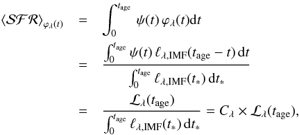
3. Although we know that no SSP luminosity ℓλ,IMF(t∗) evolves as a hat function, the hat function case shows that we cannot obtain ψ(tnow) from observations, but, at best, an average value over a time interval  . We can extend the concept of averaging the SFR over a time interval to the concept of obtaining a weighted mean of ψ(t) over any arbitrary function ϕλ(t). The only requirement is that this function is normalized over the time interval ψ(t) that is defined (i.e., tage). In the context of this paper, we can define the weight function ϕλ(t) as
 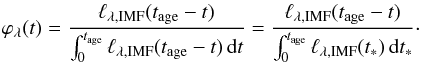 (7)The SFH ϕλ(t)-weighted mean,
  , is
, is 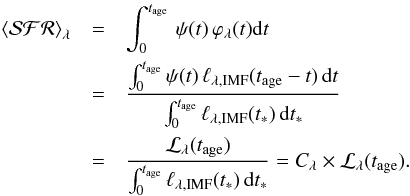 (8)The normalization coefficient of the function ϕλ(t) is the inverse of the quantity Cλ ≡ Cind used in common calibrations of the SFR. Of course, this normalization coefficient can be also interpreted as the luminosity obtained by a synthesis model under a constant SFH assumption, but
An alternative interpretation to Eq. (8) is that the observed luminosity ℒλ(tage) is the result of the SFH ψ(t) once filtered over the evolution of the luminosity produced by coeval stars ℓλ,IMF(t∗) (defined up to t∗ = tage). We can therefore obtain direct information about ψ(t) once the filter is normalized or calibrated, or, on general grounds, when the zero point of the filter is defined in a similar way as in photometric studies3.
4. The previous result is general. If we hope that  contains only information about the recent SFH, we therefore require a filter that is only sensitive to recent ages. That is, a hypothetical ℒλ(tage), whose associated ℓλ,IMF(t∗) has a zero value after some age t∗ ,ind. A break like this, if exists, can be obtained by a direct inspection of ℓλ,IMF(t∗), but also by the variation over t∗ of the integral of ℓλ,IMF(t∗). Trivially, if it goes to zero after at some t∗ ,ind value, then
 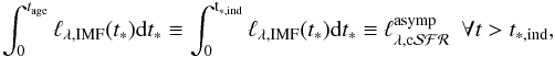 where
where 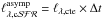 for the case of a hat function. We have kept the symbol
  to stress its similitude with the calibration constant Cind (Eqs. (3), (5), and (8)).
5. The use of the integral over t∗ instead of a direct inspection of ℓλ,IMF(t∗) would be seen as an unnecessary complication. However, the ℓλ,IMF(t∗) obtained by synthesis codes (or equivalently, the evolution of SSP models) are not hat-like functions and neither show a clear well-defined t∗ ,ind value. It shows instead that the luminosity declines with t∗ more or less quickly, depending on the wavelength. If we still aim to obtain a value that can be used as the actual for some observed ℒλ(tage) luminosity, searching for ℓλ,IMF(t∗), whose integral over time reaches a quasi-state regime, is therefore the only approach, where Δt( ≡tind) is defined by the age where this steady-state is reached.
3.2. SSP luminosity evolving as a hat function plus a power-law decay
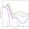 |
Fig. 1 Evolution of the slope of approximating the SSP luminosity following power-law evolution |

Characteristic quantities for ℓλ,IMF(t∗) when modeled as a power law.
1. We used a second still simplified but more realistic functional form of the SSP luminosity evolution to proceed. Assuming a properly defined zero-age main sequence, all stars increasing its luminosity (at least in UV to IR wavelengths) up to the end of the main sequence; hence any ℓλ,IMF(t∗) will have a first period with a slow increase of its luminosity at least up to the age t∗,MS where more massive stars leave the main sequence, which is typically at 3 Myr. After this age, the presence of post-main-sequence evolutionary phases results in a more complicate evolution. However, simple energetic arguments show that in a quite reasonable approximation, ℓλ,IMF(t∗) evolves as a declining power law. It is a classical result (Tinsley & Gunn 1976; Buzzoni 1995) still confirmed by comparisons with current synthesis models and proven as a useful approximation (Buzzoni 2005). For simplicity, we assumed that ℓλ,IMF(t∗) is constant in the interval [ 0,t∗,MS ] and evolves as  , from t∗,MS up to any posible tage, where ℓλ,MS is the luminosity at t∗,MS. The evolution of this SSP luminosity is
 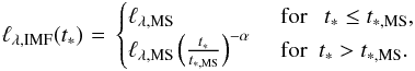 (9)As reference values, α is about equal to or lower than 1 for wavelengths longer than 3000 Å (Buzzoni 2002b). Table 1 in Buzzoni (2005) provides a detailed analysis including metallicity effects showing that the slope flattens when the metallicity decreases. As reference, we also show the evolution of α for different photometric bands obtained by the combination of different synthesis models (see Sect. 3.3 for details) in Fig. 1. In practical terms, we consider in this section generic values of α = 0.6 to 0.9 as a representation of the IR to visible bands, and α = 1.1,1.5 and larger than 2 as a generic representation of U-band, UV bands, and the number of hydrogen-ionizing photons, (Q(H), which is proportional to the emission luminosity of hydrogen recombination lines, as the Hα emission line), respectively. The numerical results obtained here assume t∗ ,MS∗,MS = 3 Myr, and, when required, tage = 13 Gyr. We show in Table 1 a more detailed version of specific values of α for different generic bands and related quantities computed using the present approximation that are discussed in this section. The lower part of the table shows α values chosen a posteriori to roughly fit the results when realistic synthesis models are used (Sect. 3.3, Table 2). We note that for Q(H) we used here a generic value of α> 2 as a limit, although a value of α = 4 would be a more realistic nominal value.
2. The integral over time of such ℓλ,IMF(t∗) for t>t∗,MS can be obtained analytically, 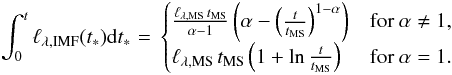 (10)This integral only has an asymptote if α> 1 with a value
 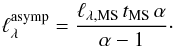 (11)The luminosity at wavelengths or bands greater than 3000 Å therefore never reach an asymptotical value, and the sensitivity of the SSP evolution of the old SFH increases as the system evolves. This situation, when translated into the statement that the time integral of the SSP luminosity reaches an asymptotic value to define a reliable SFR index situates U in a limiting situation as a result of its metallicity dependence (Buzzoni 2005). U is considered as a reliable index by some authors (e.g., Wilkins et al. 2012; Boquien et al. 2014,but see below), but not by others.
3. A direct comparison of Eqs. (10) and (11) allows evaluating the difference between the real asymptotic value and the value obtained for any chosen t provided that α> 1, hence estimating possible values of ttest where an asymptotical values has been reached. Evaluating Eq. (10) at t∗ = 13 Gyr (1 Gyr, 100 Myr), and comparing with the asymptotic value, we found that the asymptotic values are underestimated by 39% (51%, 64%) for α = 1.1 corresponding to a generic U-band. For α = 1.5 corresponding to FUV bands, the underestimation is 1% (4%, 12%). Finally, the underestimation is lower than 1. 5% in the three ages for α ≥ 2. With the exception of Q(H)-based indices (and neglecting their flattening at older ages, see Sect. 3.3 below), asymptotical values are therefore never reached given the age of the Universe. This means that
A graphical inspection of the Cind(ttest) values quoted in the appendix of Boquien et al. (2014) shows that by excluding Q(H) and apparently CFUV at some metallicities, an asymptotical value of Cind(ttest) at ttest = 1 Gyr has been not reached.
4. The fact that asymptotic values cannot be reached implies that we cannot define a characteristic timescale Δt that would allow a direct transformation of in . We stress that it is implicit in the ℓλ,IMF(t∗) evolution, which is the only filter we have to infer the SFR. However, we can try to obtain some usable summaries of ℓλ,IMF(t∗) that allow obtaining information without taking the functional form of ℓλ,IMF(t∗) explicitly into account. This is a similar problem as characterizing photometric systems or probability distributions. A typical characterization is obtained by computing cumulative distributions of the amount of flux comprised from 0 up to a given t∗ value (examples are the way SFR is calibrated; see also Leroy et al. 2012 or Johnson et al. 2013). In the following we show two alternative approaches used in the literature.
4.1. One approach is to define a mean luminosity-weighted age (Buzzoni 2002a; Boquien et al. 2014), which can be defined taking into account an assumed SFH,  (12)This can be used as a measure of the mean age of the stars that contributes to ℒλ at different wavelengths, SFH and IMF slopes (e.g., Buzzoni 2002a).
Alternatively, a characteristic weighted age of ℓλ,IMF(t∗) can be defined without considering the SFH (or, equivalently at a mathematical level, by assuming a constant SFH throughout the galaxy lifetime),  (13)which was also used by Buzzoni (2002a) and Leroy et al. (2012) to study the sensitivity of SFR to recent SFH variations, or by Boquien et al. (2014) to investigate, by comparison with ⟨t∗⟩λ,ψ(t), the stability of Cind(ttest) as a function of ttest and different SFHs. Using our power-law approximation, ⟨t∗⟩λ can easily be obtained analytically using Eq. (10), which results in values of 2.5 Gyr (937, 131, 13 Myr) for α = 0.8 (1.1, 1.5, 2). These values roughly agree with our expectations about Δt based on the stellar lifetimes that mainly contribute to different wavelengths.
The use of a simplified ℓλ,IMF(t∗) also allows easily computing the amount of sensitivity up to ⟨t∗⟩λ. We show the results in Table 1. Using first principles, given the L-shape nature of ℓλ,IMF(t∗), we can ensure that at least 50% of the sensitivity to the SFH is concentrated at ages equal to or lower than ⟨t∗⟩λ for any band (including optical ones), although the value depends α, reaching ⟨t∗⟩λ a maximum when α ~ 1.67. We therefore remark that ⟨t∗⟩λ provides valuable information, but does not provide a cutoff in ℓλ,IMF(t∗) or a characteristic time over which the recent SFH is averaged.
4.2. The evolution of SSP luminosities can also be characterized by computing the ages tλ,x% at which the sensitivity of ℓλ,IMF(t∗) to any SFH comprises x% of the total sensitivity, which is obtained by solving  (14)An advantage of tλ,x% is that it provides a more quantitative information that ⟨t∗⟩λ. Again, it cannot be taken as a general value of Δt, but at least it provides information about how much of the sensitivity of the curve would be affected by the old component of the SFH.
Using our simplified evolution of SSP luminosities, we obtain values of tλ,80% (tλ,95%) of 5.1 Gyr (10.5 Gyr) for α = 0.8, which are the generic IR/V sdss filters; 885 Myr (6.2 Gyr) for α = 1.1 or U-band; 31 Myr (375 Myr) for α = 1.5 or UV filters, and 7.5 Myr (30 Myr) for α = 2, that is, the ionizing flux (cf. Table 1). Values obtained using detailed synthesis model results are shown in Table 2 and are discussed in Sect. 3.3. We note that, given that tλ,100% = tage by construction, each tλ,x% is also a measure about how far or close we are to the physical limiting value when tλ,x% is used to define Cind. Of course, as for ⟨t∗⟩λ,ψ(t), the definition can be extended to any SFH (see Johnson et al. 2013,as an example).
5. To summarize, we described how our expectations about SFR inferences have been reduced: we first relaxed out expectations of obtaining ψ(tnow) to obtain an averaged value on a defined time interval, . But given the nature of the integrated luminosity, we needed to reduce our expectations again to obtain a where a single timescale over the SFR that has been averaged cannot be defined properly. The best we can obtain is the sensitivity of the given luminosity to the recent and old components of the global SFH. A collateral result is that this type of information can be obtained for any luminosity (not only the standard luminosities using SFH indices). When applied to optical fluxes, we obtained that 50% of the sensitivity of the integrated luminosity is concentrated at ages lower than 2 Gyr, which means that these wavelengths still contain valuable information about the recent (lower than 2 Gyr) SFH of the system. These wavelengths can be used to constrain the quality of SFR inferences obtained by bona fide indices, as we show below.
3.3. SSP luminosity evolution computed by synthesis models
1. We have used suitable examples to characterize the evolution of SSP luminosities and estimate some numbers based on an approximate formulation of the problem. We now examine the explicit computation of ℓλ,IMF(t∗). Inevitably, this implies the use of evolutionary synthesis codes to perform the detailed numerical computations, and the result becomes dependent on the details of the used code (interpolations, numerical methods, ingredients). To overcome this situation, we compiled the results of 13 different synthesis codes and stellar population results4, which are publicly available. The models include different atmosphere models5 and evolutionary tracks and isochrone sets6. We did not consider binaries, rotation, or evolution with enhanced mass-loss rates. All models assumed metallicities between 0.020 and 0.019, and used (or were transformed into) a Salpeter (1955) IMF in the mass range 0.01–100 M⊙ (the effect of variations in the IMF slope at low mass does not affect our results; we note that some models were computed with a mup = 120 M⊙, which has been taken into account in the selection of model results, see below). We did not consider nebular continuum, emission lines, or attenuation effects.
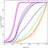 |
Fig. 2 Evolution of the sensitivity of the SSP luminosity ℓλ,IMF(t∗) with age using the upper and lower envelopes of SSP results (see text); the age (or better, age range) corresponding to a given sensibility, tλ,x% can be directly compared with the limits quoted in Table 2 for the different luminosities. In ascending ages each set of two curves corresponds to Q(H), galex/FUV and NUV, and sdss/u, g, r, i and z. These curves can also be interpreted as the evolution of synthesis models under a constant SFR assumption, except for the normalization factor. |
We used the computed low-resolution spectral energy distribution (SED) provided by each model to obtain the fluxes in Q(H), galex/FUV and NUV bands, and sdss/u, g, r, i, and z-bands7. We verified that our results are coincident with the fluxes in these bands when provided by the modeler (an exception are the results from the cmd 2.0 server, which provides the fluxes in all considered bands, except for Q(H), but not the corresponding SEDs). We discarded the age ranges of models that showed seriously discrepant results from the overall behavior of the ensemble, especially when this discrepancy was defined by the absence of particular evolutionary phases, or when the discrepant age range was outside the modeler’s expertise (which we inferred from the age range where modelers shows their results in refereed journals), and we obtained the upper and lower envelopes from the selected set of models. Then, we defined a reference SSP luminosity evolutuion ℓλ,IMF(t∗) using the linear mean value between the two envelopes. Details are presented in a companion paper (Cerviño et al., in prep.).
Characteristic quantities for ℓλ,IMF(t∗) when modeled by synthesis codes.
2. The resulting ages at which the sensitivity to the luminosity evolution of the SSP ℓλ,IMF(t∗) reaches a x% value of the total sensitivity, tλ,x%, and −log Cλ values obtained for tage = 13 Gyr are shown in Table 2. The nominal values correspond to the reference model, and the values corresponding to the upper and lower envelopes (i.e., the admissible range that encloses any public model) are quoted in brackets. The age limits quoted in Table 2 can be also obtained from Fig. 2, where we show the sensitivity evolution of the SSP luminosity ℓλ,IMF(t∗) with age using the upper and lower envelopes of SSP results (each of the envelopes was normalized to its corresponding value). These curves can also be interpreted as the evolution of synthesis models under a constant SFR assumption, except for the normalization factor. The figure shows how the dispersion in the results of different synthesis models and model ingredients propagates in tλ,x% values (or in the resulting evolution assuming a constant SFR).
The values obtained in Table 2 are comparable with tλ,90% provided in Table 1 of Kennicutt & Evans (2012) based on computations by Hao et al. (2011) and Murphy et al. (2011), although we obtain lower tλ,90% values. This is surprising because we used a much larger ttest, although tage and our SSP calibration include the emission of stellar components, which are not included in the models used by Hao et al. (2011), Murphy et al. (2011), Kennicutt & Evans (2012). This difference is probably due to the use of the Meynet et al. (1994) evolutionary tracks with enhanced mass-loss rates by the authors, the default in the starbust99 previous the release including rotation, which is not included in our calibration form selected models (see Cerviño et al., in prep. for more details).
The variability due to the use of different synthesis models in our compilation quoted in Table 2 is much lower than the 20% usually quoted in the literature. However, this scatter corresponds to an optimistic situation since our compilation is restricted to the evolutionary tracks used in common synthesis codes. A detailed analysis of possible uncertainties that are due to evolutionary tracks that are not included in our compilation can be found in Martins & Palacios (2013). In addition, the compilation only includes solar metallicity models, which means that the quoted uncertainties are again lower limits since it does not consider metallicity variations.
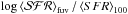
3. Figure 3 shows the ℓλ,IMF(t∗) sensitivity curves after normalizing to their integral over 13 Gyr, which is the transmission over which the SFH is seen by the corresponding luminosity. The figure allows a direct comparison with the sensitivity to the SFH for each possible integrated luminosity, regardless of whether it is used as a recent SFH proxy or not. To simplify the discussion, we only used the reference model described before. The left panel in the figure shows the sensitivity on a linear scale form 0 to 10 Myr, the right panel shows the sensitivity on a logarithmic scale throughout the whole age range. In the following paragraphs we compare the four index groups with different behavior, which are Q(H), UV indices, U (sdss/u), and optical/ IR indices.
Q(H) is clearly the index most sensitive to the younger component of the SFH. Even more, the sensitivity peaks at ages lower than 1 Myr, hence, at first approximation, it almost reproduces the current SFH value. In addition, its sensitivity to the recent SFH (tnow − 3 Myr) is higher by about a factor 3 than any other index. It is the least sensitive index to the SFH at ages tnow − 10 Myr up to ages older than 1 Gyr, where the sensitivity of galex/FUV is lower. The dynamic range of the sensitivity to the SFH at different ages covers six decades (more than three decades in the first 10 Myr), hence, it is quite stable8 to large-scale variations in the SFH at ages older than 50 Myr. In a relative comparison with the other indices (i.e., where the different sensitivities cross each other), Q(H) is more sensitive to the SFH at ages lower ~4 Myr than galex filters, ~5 Myr than u, and ~7 Myr than optical bands.
The indices based on the UV, galex/FUV and NUV have a quite similar transmission, although galex/FUV is slightly more sensitive to the young component up to ages around 8 Myr than galex/NUV, and galex/NUV is more sensitive than galex/FUV for the SFH at ages older than 100 Myr. The peak of the sensitivity is around 3 Myr (the value of tMS at the given metallicity); the sensitivity of both indices is broader than Q(H) and extends with an apreciable sensitivity for ages older than 10 Myr. Both indices have an almost equivalent sensitivity to the SFH in the range 8 to ~50 Myr. At older ages, and especially at ages older than ~300 Myr, the sensitivity of galex/FUV drops abruptly, whereas the one of galex/NUV declines more smoothly. The dynamic range of the sensitivity at different ages covers almost five decades (more than three decades in the first 500 Myr), and, as for Q(H), both indices are quite robust to large-scale variations of the SFH, although at a timescale much longer that the one associated with Q(H).
The U-band is an intermediate case between optical and UV bands. It is about a factor 2 less sensitive to the recent SFH than UV filters, but still a factor 2 higher than g; however, the sensitivity to the SFH after 50 Myr is higher than the UV bands (reaching factors higher than 10 at ages older than 2–3 Gyr). Although apparently it is a correct recent SFR index using the standard method when tested over short timescales (i.e., ttest up to ~100 Myr), it behaves more like optical colors at older ages. The slope of the sensitivity curve is quite similar to −1, which is the limiting case where the sensitivity to young and old components of the SFH is similar. The dynamic range of the sensitivity is slightly longer than three decades over the whole age range, and, as quoted before, more sensitive to large-scale variations of the SFH than the previous indexes.
Longer wavelengths (g, r, i, and z-bands) still show a high sensitivity to the recent SFH, however, their dynamic range is shorter than three decades, hence it is much more affected by large-scale variations on the SFH. In addition, the sensitivity curves of all optical bands intercept each other near 1 Gyr. Of these, the sensitivity of the r, i, and z-bands is quite similar, which implies at first approximation that they provide redundant information in any SFH inference, especially after the first 10 Myr.
3.3.1. Relative timescales and corrections
1. In the previous section we showed the difficulties of defining any characteristic timescale Δt that allows transforming an observed into  or at least to obtain an age interval over which the SFH has been averaged. We can choose characteristic timescales associated with the evolution of SSP luminosities ℓλ,IMF(t∗) (e.g., ⟨t∗⟩λ, any tλ,x% or any other related timescale), but they do not directly provide the time range over which the actual SFH is averaged either ⟨t∗⟩λ,ψ, or tλ,x%,ψ, which depends on the unknown functional form of the overall SFH.
However, by the comparing the obtained for different indices (including optical ones), we can obtain relative timescales of the SFH regardless of its functional form. This means that we cannot define the time interval over which ψ(t) is averaged, but we can establish some characteristic times which, after they are compared with an associated color, allows establishing the relative strength of ψ(t) after and before this time. As result, although we cannot correct to obtain , we can establish whether tλ,x%,ψ (which is unknown) is longer or shorter than tλ,x%. In the following we assume the general result that the sensitivity to the recent SFR increases at lower wavelengths.
2. Relative timescales are given by the intersection of the different transmission curves: we assumed two indices Cℬ and Cℛ where ℬ and ℛ refer to the bluest or reddest bands used to define the color, or in terms of the transmission curves, more sensitive to the young (ℬ) or old (ℛ) component of the SFH. First, we defined a reference color (ℬ − ℛ)ref obtained from the corresponding Cλ values (i.e., obtained at tage). Second, t∗ ,ℬℛ is the intersection age of the two sensitivity curves. Given that ψ(t) is independent of the transmission curves, an extinction-corrected observed color bluer than (ℬ − ℛ)ref implies that ψ(t) has a stronger contribution in the age region where the blue index is more sensitive, that is, at ages younger than t∗ ,ℬℛ. In this situation, we can also ensure that any of the timescales ⟨t∗⟩λ or tλ,x% are upper values of the actual ⟨t∗⟩λ,ψ(t) or tλ,x%,ψ(t) values. That is, from the variation of the color (ℬ − ℛ) with respect to (ℬ − ℛ)ref we can obtain information about the relation between ⟨t∗⟩λ (obtained theoretically) and ⟨t∗⟩λ,ψ(t) (the quantity we are interested in).
This case can be viewed as the comparison of the colors obtained from a constant SFH over all the possible age range with any other possible SFH. The improvement is that we have taken advantage of the functional form of the different normalized ℓλ,IMF(t∗) curves and their intersection in the time axis to characterize the deviations from a constant SFH.
We illustrate this with an example: Q(H) is not directly an observable, but it is directly proportional to the Hα emission line with a conversion factor of 1.36 × 10⁻¹², (assuming case B recombination and no escape of ionizing photons, hence an upper limit of L(Hα)). Using the flux in r band as a representation of the continuum near Hα, the resulting equivalent width of Hα in emission obtained from the respective CQ(H) and Cr values is EW(Hα) ~ 45 Å. We note that in this computation the value of r is a lower limit since we did not consider nebular contribution to r (which is about 40% at young ages, according to Mas-Hesse & Kunth 1991), therefore 45 Å is a maximum value. Since the sensitivity curves of Q(H) and r cross at around 7 Myr, the actual SFH must be stronger (compared to a constant SFH) in the last 7 Myr when EW(Hα) > 45 Å. A higher value of EW(Hα) implies that recent SFH is more concentrated at younger ages, hence the mean luminosity-weighted age associated with the actual SFH ⟨t∗⟩ψ(t) is lower than the mean luminosity-weighted age associated with a constant SFH ⟨t∗⟩, hence the recent SFH is bursty-like (at least at first approximation). However, the inverse reasoning of a recent SFH extending in time for ages older than 7 Myr if EW(Hα) < 45 Å is not true since it can be due to the enhancement of r by nebular emission (we did not consider), or the leaking of ionizing photons. Regardless, the EW(Hα) value and the normalized ℓλ,IMF(t∗) curves provide additional information about the recent SFH, which helps to interpret the quantity  independently of the SFH itself. Equivalently, FUV-NUV colors higher (or lower) than −0.02 or NUV-r higher or lower than 1.57 provide additional constraints about the timescales around 7–50 Myr and 140 Myr, respectively (cf. Table 3).
AB colors and characterisitcs ages for calibration.
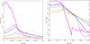 |
Fig. 3 SSP luminosity evolution ℓλ,IMF(t∗) as SFH sensitivity curve (i.e., after normalizing to the integral of the SSP over the age of the system, 13 Gyr in our case). The left panel shows the sensitivity curve on a linear scale from 0 to 107 yr, the right panel the sensitivity curve on a log-log scale for the whole age range. In descending order at young ages the curves correspond to Q(H), galex/FUV and NUV, and sdss/u, g, r, i and z. |
3. In the previous paragraph we focused on providing a timescale for the obtained from data of a single system. For a large set of systems (e.g., survey studies), the principal interest is not the timescale associated with the in each system, but the comparison of , where Δt is equal to (or at least similar to) all the systems in the set. In this case, the comparison of the observed color (ℬ − ℛ) with respect to (ℬ − ℛ)ref provides a hint about the correction needed to transform into .
4. However, although the idea is formally correct, this method only provides first-order timescales. As an example, the galex/FUV and NUV sensitivities cross each other nominally at 17 Myr, but the sensitivity is almost identical (with variations lower than ±10%) in the age range from 7 to 50 Myr9. In addition, the present sensitivity curves have been obtained assuming that all stars formed in the past 13 Gyr have solar metallicity, which neglects metallicity evolution of different populations. Finally, we did not consider extinction effects, which affect the results of SFR inferences and which have been studied by different authors. With these caveats, we show in Table 3 the (ℬ − ℛ)ref colors associated with the different Cind values of Table 2 when expressed in AB magnitudes and the approximate ages (obtained by by-eye inspection of Fig. 3) where the sensitivity curves cross each other.
5. Finally, we stress that our results are independent of the SFH and also apply to the extreme SFH of instantaneous bursts of star formation. As an example, an EW(Hα) > 45 Å roughly corresponds to a burst (i.e., SSP) younger than 7 Myr. A direct implication is that, in practice, we can interpret any fit of colors obtained from SFR indices to SSP results as an indication of the different timescales each index applies. Although this is beyond the scope of this paper, such an alternative vision about what provides a SSP fit, even when we know a priori that our studied system is not a single burst of star formation, can be potentially exploited in SFH inferences obtained from the integrated spectra or photometry of any stellar system.
4. Discussion by comparison with other works
The principal result of this work is a change of perspective about what is obtained in recent SFH inferences. This result has no great impact on the final values of the standard SFR calibrations (Q(H) and UV indices), which are only affected to a few percent, but it clearly affects the U-band and allows introducing optical colors as a cross-check of the timescales associated with SFR inferences. Although we have obtained some numbers, our approach is rather qualitative. However, these quantitative results allow placing on a firm theoretical bases some recent results related with recent SFH inferences. Instead of performing a quantitative test, we use the results by other authors to discuss our main results.
1. Extending the results of Boquien et al. (2014). The first result refers to the age ttest that should be used to calibrate recent SFH indices. As we showed, the best ttest value is the age of the galaxy under consideration tage (which is redshift dependent). This applies even to SFR inferences in regions inside galaxies, since it is always possible that an old stellar population contributes.
Taking this into consideration, we can extend the results obtained by Boquien et al. (2014) about the use of any particular ttest: Boquien et al. (2014) used the SFH from MIRAGE simulations (Perret et al. 2014) covering ages up to 780 Myr and compared the instantaneous SFH with the evolution of for different indices (Q(H), FUV, NUV, and u) obtained by including the simulated SFH in stellar population synthesis codes. Their main finding is that the calibration of the SFR is age dependent (which is in line with our claim that the best ttest is the age of the system), and they proposed using a ttest of at least 1 Gyr instead of the typical one of 100 Myr when a fixed value of ttest is used. We note that 1 Gyr is almost the maximum age considered by the SFH they used.
However, we can also establish that by extending the simulations over wider age range, a calibration over ttest = 1 Gyr will again produce biased results (see Sect. 3.2). In particular, the u band is especially ill defined as SFR index: since it evolves as a power law with a slope close to the limiting value of −1, it would appear to be a good SFR index for any fixed age ttest, but it overestimates the true SFR if the system is older than ttest.
In addition, Boquien et al. (2014) studied the delay between ψ(t) and the produced by the models at the given t. They found that follows ψ(t) with a delay of about 1 Myr, whereas the other indices have typical delays of a few Myr, although their plots (e.g., Figs. 6 and 8) show a delay plus a smoothness effect. These results are, again, fully consistent with our analysis that is a filter over ψ(t).
2. Results of Johnson et al. (2013). A second result is to break the artificial duality in the use of ttest, which is implicitly assumed to be related with a possible value of tind, that is, the timescale over the SFR is averaged. We have shown that these timescales cannot be obtained because they depend on the particular SFH, which is unknown. Moreover, to impose a constant SFH ad hoc to obtain a tind value produces ill-defined questions because tind is intrinsically undefined. This situation is clearly illustrated in Johnson et al. (2013), who, making use of an SFH obtained from CMD, computed the SFH-dependent tuv,80%,ψ(t) values from a sample of 50 nearby dwarf galaxies (where uv refers to both FUV and NUV). They found that depending on the SFH, such values range from a few Myr up to 10 Gyr, which value is linearly correlated with the NUV-r color, so that the inferred  cannot be univocally related with any SFR timescale.
We stress that this result is not a problem of the calibrations of the recent SFR, but rather of the interpretation of what we would like a value to provide, but it does not. Again, the calibrations are correct (when ttest = tage, a question also addressed partially in Johnson et al. 2013), but these calibrations do not provide a timescale directly. Additional information (such as optical or IR colors) is necessary to provide a recent SFR timescale (information about the global SFH). As an example, our computations produce a NUV-r = 1.57 (cf. Table 3) with a characteristic age associated with such a color around 180 Myr. In the previous section we stated that a bluer (redder) NUV-r indicates that the SFH is more concentrated at younger (older) ages, which translates into a lower (higher) value of any tuv,x%,ψ(t) characteristic age. This effect agrees with the findings of Johnson et al. (2013).
However, we note that our explanation of the correlation between NUV-r and tuv,80%,ψ(t) found by Johnson et al. (2013) is only valid for a NUV-r color bluer or near a NUV-r value of 1.57, but it cannot extend to extreme (much redder than 1.57) NUV-r colors. That is, we only explain the bluer part of the correlation found by Johnson et al. (2013), but a more complete study about the impact of the SFH at old ages (roughly, older than 1 Gyr) is required to find a satisfactory explanation of the correlation.
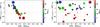 |
Fig. 4 Ratio of |
3. Results of Simones et al. (2014). For star-forming regions inside a galaxy we have a similar situation of a correlation of different colors with any SFR averaged over a predefined timescale, although with some subtle differences: (a) Stellar populations formed at old ages will be spread throughout the volume of the galaxy, hence, it is expected that ψ(t)region that would be obtained from particular blue region will have a lower contribution from the older stellar populations (depending on the position in the galaxy). (b) Although the increasing resolution would optimize a ψ(t)region inference, it also implies a reduction in the amount of stars, which contributes to the total luminosity, therefore an increasing on the uncertainty of the inferences obtained from the integrated luminosity (the so-called IMF sampling effects, although stellar luminosity function sampling effects is a more correct description; see Cerviño & Luridiana 2004, 2006; Cerviño 2013, and references therein for an extensive discussion of the subject).
We illustrate both situations using the work by Simones et al. (2014), who analyzed the CMDs obtained from the Panchromatic Hubble Andromeda Treasury data (Dalcanton et al. 2012) to obtain the corresponding SFH in the past 500 Myr, and the extinction of 33 FUV-bright regions in M31 and used them to test the reliability of the FUV as an SFR index at small scales.
The authors provided the SFH of each region. From this, they obtained the SFH averaged over the past 100 Myr (⟨SFR⟩100), the age where the SFH has a peak, agepeak, and the ratio between the mass of stars formed in the agepeak over the mass of stars formed in the past 100 Myr, Mpeak/M100. In addition, they used the SFH as input of a synthesis model to obtain the integrated luminosity in galex/FUV and (FUV-NUV)mod color, and the corresponding  using the standard calibration. Finally, they used their extinction solution and applied it to galex data to obtain the extinction-corrected FUV flux and the corresponding
  . One of the advantages of this paper is that in addition to their detailed analysis, the authors provided a plot of the SFHs obtained from each of the studied regions as well as a different set of tables including the computed quantities, from which not tabulates values such as the extinction-corrected (FUV-NUV)obs,0 color, can be obtained. From a comparison of the ratio
 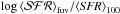 as a function of the area covered by the region, and using observed and modeled
  values, they claimed that the extinction-corrected FUV fluxes are, on average, consistent with ⟨SFR⟩100 within a 1-σ scatter, which is related with the discrete sampling of the IMF and the high time variability on the recent SFH.
Again we can extend the conclusions of Simones et al. (2014) by taking advantage of the present study. In Fig. 4 we show the ratio vs. the FUV-NUV color obtained from Simones et al. (2014) by the use of the SFH implemented in synthesis models (left), and obtained from the observed data after correcting for extinction (right). The color of the different points shows the agepeak value, and the size of each point is proportional to Mpeak/M100.
When synthesis models are used and sampling effects are neglected, , the FUV-NUV color, and agepeak are clearly correlated. This is stronger for larger Mpeak/M100. The combination of agepeak and Mpeak/M100 are a measure of the concentration of the SFH at different ages, therefore the results of their simulations are consistent with our prediction about the dependence of , ⟨SFR⟩Δt, and the color of the system. We note that Simones et al. (2014) concluded that the dispersion on  is due to the variability of the recent SFH, but they are unaware about the correlation shown here and that this correlation can be used to reduce the scatter.
When observational data are used, sampling effects may cause the correlation of and the FUV-NUV color to disappear. This result is expected because only one cluster in their analysis reaches an amount of gas transformed into stars in the past 100 Myr larger than 105M⊙, and this value is approximately the lowest limit quoted by Cerviño & Luridiana (2004) as necessary to model a system safely in UV-optical bands (i.e., without extreme sampling effects where the mean value obtained by synthesis models loses its predictive power). However, there is still a clear tendency of found lower values of in clusters where the SFH has a higher star formation concentration at older ages and vice versa. This means that  still depends on the age range in which the actual SFH is more concentrated.
5. Conclusions
We here translated the statements quoted in the constant SFR approximation presented by Kennicutt (1998), which require synthesis models for its calibration, to the intrinsic algebra of synthesis models to capture the principal characteristics of such an approximation, which allows obtaining reasonable SFR inferences. The results obtained from this study are listed below.
-
1.
When expressed in terms of SFH studies, any in-tegrated luminosity can be (and should be) con-sidered as the result of filtering the SFH using SSP.
 (15)where
Cλ, the SFR
calibration coefficient, is a normalization factor of SSP models.
(15)where
Cλ, the SFR
calibration coefficient, is a normalization factor of SSP models. -
2.
Given that all the SFH of the system must be taken into account, the most reliable choice of the age to be used in the calibration is the system age, tage (roughly 13 Gyr at z = 0). This calibration varies with the redshift, provided the assumption is correct that all galaxies have been formed at a given cosmic epoch and independently of their posterior SFH.
-
3.
The time evolution of the SSP luminosity ℓλ,IMF(t) from 0 to tage acts like a filter over the SFH, therefore the characterization of ℓλ,IMF(t) enables us to infer the recent SFR. From this perspective, there is no requirement about the functional form of the SFH to calibrate different SFR indices; in particular, a constant SFR is not a required hypothesis.
-
4.
Using a simple parametrization of the SSP luminosity evolution ℓλ,IMF(t) and detailed synthesis models results, we found that U band is an ill-defined index to be used as a primary proxy of the SFR. It appears to be a primary proxy (Q(H) or UV indices) when the calibration is done using short timescales, and to be an optical index when long timescales are used. However, this situation does not pose any problem if tage is used as calibration age.
-
5.
We showed that the assumed requirement that the integrated luminosity reach an asymptotical or steady-state value under a constant SFR hypothesis is not needed. For the given age of the Universe, such an asymptotical value is never reached. Reaching the asymptotical value would allow defining a practical cutoff in the sensitivity defined by ℓλ,IMF(t), hence defining a characteristic timescale over the SFH is in practice averaged. Unfortunately, such a cutoff does not exist, and characteristic timescales are dependent on the unknown SFH. The best we can do is to characterize the sensitivity to the SFH provided by ℓλ,IMF(t). We showed that the time used for the calibration must be not confused with the characteristic timescales of ℓλ,IMF(t), which are strongly dependent on the wavelength. We provided different ways to obtain such characteristic timescales.
-
6.
Using the
values obtained from different indices and the characterization ℓλ,IMF(t)
(e.g., the use of equivalent widths or colors), we can establish time ranges where the
SFH contributes more strongly to the different indices, hence improves the meaning of
the measure given by .
The results obtained in this way are independent of the functional form of the SFH. To
perform this task, it is required to calibrate all possible wavelengths (not only the
standard ones of ionizing flux or UV fluxes), as established by Eq. (15). -
7.
We showed that, theoretically, there should be a correlation between the SFR obtained by the calibration of a particular luminosity
,
the physical SFR that is the SFH averaged over a given time interval
,
and the galaxy colors. This correlation is present in other works in the literature,
and it is generally considered has proof of the different timescales associated with
and ,
hence it is a problem to obtain .
We showed that it is a natural result implicit in the very nature of the relation of
the observed luminosity and the SFH of the system, and that it can be used to correct
for (or at least estimate a correction of) the
to obtain .
After this study we conclude that the constant SFR approximation quoted by Kennicutt (1998) contains deeper implications that are intrinsic to the population synthesis model algebra, but with a different wording and a few subtle changes: (1) the quoted constant SFH assumption is naturally translated into a normalization factor to express SSP results as a sensitivity curve, and it is applicable to any wavelength. (2) The steady-state (i.e., asymptotic) requirement to define a reliable SFR is naturally translated into a measure of the relative sensitivity of the ℓλ,IMF(t) filter to the young and old component of the SFH, and, although a desirable property, it is not a requirement to obtain information about the recent SFH. (3) Finally, the bluest and best statement is a synthetic and operative version of the fact that regardless of wavelength, a sensitivity peak occurs in the recent SFH age range. Since shorter wavelengths have a higher sensitivity, a blue color ensures that the possible contamination from the old component of the SFH is minimized. However, this statement has a limit depending on the galaxy color and the studied system; it is applicable to systems with colors redder than the colors associated with the calibration of ℓλ,IMF(t) (or equivalently, predictions of a constant SFH throughout the possible age range). For extreme blue colors, a first-order correlation within color was found, the obtained value of and the actual value of . It is unclear whether this correlation can be used to transform value into the desired value of , but at least it provides and indication about over- or underestimations of with respect to .
As a final comment, this work has been done in an old-fashioned way, preferring the use of reasonable analytical approximations as a function of suitable parameters to the use of detailed numerical computations where numerical values make any possible parametrization difficult. This reasoning, although not exact, can be found in most papers of B. Tinsley and A. Buzzoni, who showed that the key points to understand the results obtained by detailed simulations can be obtained using simple, but powerful, reasoning. As we showed, this method indicates which types of plots or correlations might be hidden under more elaborate numerical experiments. It is true that for some aspects (track interpolations and atmosphere model assignation, among others) synthesis models should be used as black boxes for non-initiated developers, but for some purposes a simple inspection of the implicit equations in any synthesis model, and their possible solutions, is the only requirement.
This should read ℓλ(m,t∗,Z,Ω), where Z is the initial metallicity of the star and Ω its rotational velocity, which implies that the corresponding parameters are included in the stellar birth-rate. In addition, interactions between stars (i.e., binary interactions) can also be considered, which depend on additional parameters that, again, must be included in the stellar birth-rate. We neglect all such additional parameters throughout.
The time dependence of the luminosity is used in works studying the star formation process itself, where different classes of YSO are considered; see Lada et al. (2013), Román-Zúñiga et al. (2015) as examples.
The analogy of synthesis models results and photometry is known and is quoted by Shore (2002); surprisingly, this analogy has been poorly explored in the literature and is typically limited to restricted ttest values; however, see Otí-Floranes & Mas-Hesse (2010), Leroy et al. (2012) as counterexamples, who used ℓλ,IMF(t) as SFH-sensitivity curve.
The used models are starbust99 (Leitherer et al. 1999, 2014), galev (Kotulla et al. 2009), galaxev (Bruzual & Charlot 2003, version 2012), pegase2.0 (Fioc & Rocca-Volmerange 1997; Fioc & Rocca-Volmerange 1999), popstar (Mollá et al. 2009; Martín-Manjón et al. 2010; García-Vargas et al. 2013), fsps (Conroy et al. 2009, 2010; Conroy & Gunn 2010), galadriel Tantalo & Chiosi (2004), bpass (Eldridge & Stanway 2009, 2012, in its single star version), sed@ (Mas-Hesse & Kunth 1991; Cerviño & Mas-Hesse 1994; Cerviño et al. 2002), models provided by C. Maraston (Maraston 1998, 2005) and A. Buzzoni (Buzzoni 1989) with different horizontal branch morphologies, models from the batsi web server including different α-enhancement factors (Percival et al. 2009; Pietrinferni et al. 2009; Salaris et al. 2010), and models from the cmd 2.0 web server (Padova models, Girardi et al. 2002; Girardi et al. 2008; Marigo et al. 2008). The web addresses of the models can be found in http://sedfitting.org.
Atmosphere models include grids by Kurucz (1991), Castelli et al. (1997), different versions of the basel libraries (Lejeune et al. 1997, 1998; Westera et al. 2002) for normal stars, the grids by Schmutz et al. (1992), CoStar (Schaerer & De Koter 1997) and Smith et al. (2002), for massive and WR stars, and Planck functions and Rauch (2003) models for white dwarfs (WD).
The tracks and isochrones used by the different models models are the Geneva tracks (Schaller et al. 1992), Padova tracks (Bertelli et al. 1994; Girardi et al. 2000; Marigo & Girardi 2007), batsi tracks (Pietrinferni et al. 2004, 2006; Cordier et al. 2007; Percival et al. 2009; Pietrinferni et al. 2009; Salaris et al. 2010), and Paczyński (1970, 1975), Bloecker (1995), Vassiliadis & Wood (1994) for post-AGB/WD evolution.
Filter transmission curves have been taken from the Spanish virtual observatory, SVO, server at http://svo2.cab.inta-csic.es/theory/fps3/
Numerical computations shows that assuming tage = 13 Gyr, the old component of exponential decay and delayed SFH with τ> 3 Gyr affects the index by less than 10% (Cerviño et al., in prep.).
These numbers were obtained without considering the uncertainties in our calibration of synthesis models, which introduces an additional scatter in the reliable timescales.
Acknowledgments
We thank the referee, Rob Kennicutt, for his comments, which helped improve this paper. This work has made extensive use of TopCat software (Taylor 2005), and we acknowledge Mark Taylor for its development. This work has been supported by the Spanish Programa Nacional de Astronomía y Astrofísica of the MINECO by the projects AYA2014-58861-C3-1 (MC), and AYA2013-42781-P (SH), and partially supported by the project AYA2011-C03-01 (AB).
References
- Bertelli, G., Bressan, A., Chiosi, C., Fagotto, F., & Nasi, E. 1994, A&AS, 106, 275 [NASA ADS] [Google Scholar]
- Bloecker, T. 1995, A&A, 299, 755 [NASA ADS] [Google Scholar]
- Boquien, M., Buat, V., & Perret, V. 2014, A&A, 571, A72 [NASA ADS] [CrossRef] [EDP Sciences] [Google Scholar]
- Bruzual, A. G., & Charlot, S. 2003, MNRAS, 344, 1000 [NASA ADS] [CrossRef] [Google Scholar]
- Buzzoni, A. 1989, ApJS, 71, 817 [NASA ADS] [CrossRef] [Google Scholar]
- Buzzoni, A. 1995, ApJS, 98, 69 [NASA ADS] [CrossRef] [Google Scholar]
- Buzzoni, A. 2002a, in New Quests in Stellar Astrophysics: the Link Between Stars and Cosmology, 189 [Google Scholar]
- Buzzoni, A. 2002b, AJ, 123, 1188 [NASA ADS] [CrossRef] [Google Scholar]
- Buzzoni, A. 2005, MNRAS, 361, 725 [NASA ADS] [CrossRef] [Google Scholar]
- Calzetti, D. 2013, in Secular Evolution of Galaxies, eds. J. Falcón-Barroso, & J. H. Knapen, Secular Evolution of Galaxies (Cambridge: Cambridge University Press), 419 [Google Scholar]
- Castelli, F., Gratton, R. G., & Kurucz, R. L. 1997, A&A, 318, 841 [NASA ADS] [Google Scholar]
- Cerviño, M. 2013, New Astron. Rev., 57, 123 [NASA ADS] [CrossRef] [Google Scholar]
- Cerviño, M., & Luridiana, V. 2004, A&A, 413, 145 [NASA ADS] [CrossRef] [EDP Sciences] [Google Scholar]
- Cerviño, M., & Luridiana, V. 2006, A&A, 451, 475 [NASA ADS] [CrossRef] [EDP Sciences] [Google Scholar]
- Cerviño, M., & Mas-Hesse, J. M. 1994, A&A, 284, 749 [NASA ADS] [Google Scholar]
- Cerviño, M., Mas-Hesse, J. M., & Kunth, D. 2002, A&A, 392, 19 [NASA ADS] [CrossRef] [EDP Sciences] [Google Scholar]
- Conroy, C. 2013, ARA&A, 51, 393 [NASA ADS] [CrossRef] [Google Scholar]
- Conroy, C., & Gunn, J. E. 2010, ApJ, 712, 833 [NASA ADS] [CrossRef] [Google Scholar]
- Conroy, C., Gunn, J. E., & White, M. 2009, ApJ, 699, 486 [NASA ADS] [CrossRef] [Google Scholar]
- Conroy, C., White, M., & Gunn, J. E. 2010, ApJ, 708, 58 [NASA ADS] [CrossRef] [Google Scholar]
- Cordier, D., Pietrinferni, A., Cassisi, S., & Salaris, M. 2007, AJ, 133, 468 [NASA ADS] [CrossRef] [Google Scholar]
- Dalcanton, J. J., Williams, B. F., Lang, D., et al. 2012, ApJS, 200, 18 [NASA ADS] [CrossRef] [Google Scholar]
- Eldridge, J. J., & Stanway, E. R. 2009, MNRAS, 400, 1019 [NASA ADS] [CrossRef] [Google Scholar]
- Eldridge, J. J., & Stanway, E. R. 2012, MNRAS, 419, 479 [NASA ADS] [CrossRef] [Google Scholar]
- Evans, N. J. I., Dunham, M. M., Jørgensen, J. K., et al. 2009, ApJS, 181, 321 [NASA ADS] [CrossRef] [Google Scholar]
- Fioc, M., & Rocca-Volmerange, B. 1997, A&A, 326, 950 [NASA ADS] [Google Scholar]
- Fioc, M., & Rocca-Volmerange, B. 1999, ArXiv e-prints [arXiv:astro-ph/9912179] [Google Scholar]
- García-Vargas, M. L., Mollá, M., & Martín-Manjón, M. L. 2013, MNRAS, 432, 2746 [NASA ADS] [CrossRef] [Google Scholar]
- Girardi, L. A., Bressan, A., Bertelli, G., & Chiosi, C. 2000, A&AS, 141, 371 [NASA ADS] [CrossRef] [EDP Sciences] [Google Scholar]
- Girardi, L. A., Bertelli, G., Bressan, A., et al. 2002, A&A, 391, 195 [NASA ADS] [CrossRef] [EDP Sciences] [Google Scholar]
- Girardi, L., Dalcanton, J., Williams, B., et al. 2008, PASP, 120, 583 [NASA ADS] [CrossRef] [Google Scholar]
- Hao, C.-N., Kennicutt Jr., R. C., Johnson, B. D., et al. 2011, ApJ, 741, 124 [NASA ADS] [CrossRef] [Google Scholar]
- Hirashita, H., Buat, V., & Inoue, A. K. 2003, A&A, 410, 83 [NASA ADS] [CrossRef] [EDP Sciences] [Google Scholar]
- Johnson, B. D., Weisz, D. R., Dalcanton, J. J., et al. 2013, ApJ, 772, 8 [NASA ADS] [CrossRef] [Google Scholar]
- Kennicutt, Jr., R. C. 1998, ARA&A, 36, 189 [Google Scholar]
- Kennicutt, Jr., R. C., & Evans, N. J. 2012, ARA&A, 50, 531 [NASA ADS] [CrossRef] [Google Scholar]
- Kotulla, R., Fritze, U., Weilbacher, P., & Anders, P. 2009, MNRAS, 396, 462 [NASA ADS] [CrossRef] [Google Scholar]
- Kurucz, R. L. 1991, in NATO Advanced Science Institutes (ASI) Series C, eds. L. Crivellari, I. Hubeny, & D. G. Hummer, 341, 441 [Google Scholar]
- Lada, C. J., Lombardi, M., Román-Zúñiga, C., Forbrich, J., & Alves, J. F. 2013, ApJ, 778, 133 [NASA ADS] [CrossRef] [Google Scholar]
- Leitherer, C., Schaerer, D., Goldader, J. D., et al. 1999, ApJS, 123, 3 [NASA ADS] [CrossRef] [Google Scholar]
- Leitherer, C., Ekstrom, S., Meynet, G., et al. 2014, ApJS, 212, 14 [NASA ADS] [CrossRef] [Google Scholar]
- Lejeune, T., Cuisinier, F., & Buser, R. 1997, A&AS, 125, 229 [NASA ADS] [CrossRef] [EDP Sciences] [Google Scholar]
- Lejeune, T., Cuisinier, F., & Buser, R. 1998, A&AS, 130, 65 [NASA ADS] [CrossRef] [EDP Sciences] [Google Scholar]
- Leroy, A. K., Bigiel, F., de Blok, W. J. G., et al. 2012, AJ, 144, 3 [NASA ADS] [CrossRef] [Google Scholar]
- Madau, P., & Dickinson, M. E. 2014, ARA&A, 52, 415 [NASA ADS] [CrossRef] [Google Scholar]
- Maraston, C. 1998, MNRAS, 300, 872 [NASA ADS] [CrossRef] [Google Scholar]
- Maraston, C. 2005, MNRAS, 362, 799 [NASA ADS] [CrossRef] [Google Scholar]
- Marigo, P., & Girardi, L. 2007, A&A, 469, 239 [NASA ADS] [CrossRef] [EDP Sciences] [Google Scholar]
- Marigo, P., Girardi, L. A., Bressan, A., et al. 2008, A&A, 482, 883 [NASA ADS] [CrossRef] [EDP Sciences] [Google Scholar]
- Martín-Manjón, M. L., García-Vargas, M. L., Mollá, M., & Díaz, A. I. 2010, MNRAS, 403, 2012 [NASA ADS] [CrossRef] [Google Scholar]
- Martins, F., & Palacios, A. 2013, A&A, 560, A16 [NASA ADS] [CrossRef] [EDP Sciences] [Google Scholar]
- Mas-Hesse, J. M., & Kunth, D. 1991, A&AS, 88, 399 [NASA ADS] [Google Scholar]
- McKee, C. F., & Ostriker, E. C. 2007, ARA&A, 45, 565 [NASA ADS] [CrossRef] [Google Scholar]
- Meynet, G., Maeder, A., Schaller, G., Schaerer, D., & Charbonnel, C. 1994, A&AS, 103, 97 [Google Scholar]
- Mollá, M., García-Vargas, M. L., & Bressan, A. 2009, MNRAS, 398, 451 [NASA ADS] [CrossRef] [Google Scholar]
- Murphy, E. J., Condon, J. J., Schinnerer, E., et al. 2011, ApJ, 737, 67 [NASA ADS] [CrossRef] [Google Scholar]
- Otí-Floranes, H., & Mas-Hesse, J. M. 2010, A&A, 511, A61 [NASA ADS] [CrossRef] [EDP Sciences] [Google Scholar]
- Paczyński, B. 1970, Acta Astron., 20, 47 [NASA ADS] [Google Scholar]
- Paczyński, B. 1975, ApJ, 202, 558 [NASA ADS] [CrossRef] [Google Scholar]
- Percival, S. M., Salaris, M., Cassisi, S., & Pietrinferni, A. 2009, ApJ, 690, 427 [NASA ADS] [CrossRef] [Google Scholar]
- Perret, V., Renaud, F., Epinat, B., et al. 2014, A&A, 562, A1 [NASA ADS] [CrossRef] [EDP Sciences] [Google Scholar]
- Pietrinferni, A., Cassisi, S., Salaris, M., & Castelli, F. 2004, ApJ, 612, 168 [NASA ADS] [CrossRef] [Google Scholar]
- Pietrinferni, A., Cassisi, S., Salaris, M., & Castelli, F. 2006, ApJ, 642, 797 [NASA ADS] [CrossRef] [Google Scholar]
- Pietrinferni, A., Cassisi, S., Salaris, M., Percival, S., & Ferguson, J. W. 2009, ApJ, 697, 275 [NASA ADS] [CrossRef] [Google Scholar]
- Rauch, T. 2003, A&A, 403, 709 [NASA ADS] [CrossRef] [EDP Sciences] [Google Scholar]
- Román-Zúñiga, C. G., Ybarra, J. E., Megías, G. D., et al. 2015, AJ, 150, 80 [NASA ADS] [CrossRef] [Google Scholar]
- Salaris, M., Cassisi, S., Pietrinferni, A., Kowalski, P. M., & Isern, J. 2010, ApJ, 716, 1241 [NASA ADS] [CrossRef] [Google Scholar]
- Salpeter, E. E. 1955, ApJ, 121, 161 [Google Scholar]
- Schaerer, D., & De Koter, A. 1997, A&A, 322, 598 [NASA ADS] [Google Scholar]
- Schaller, G., Schaerer, D., Meynet, G., & Maeder, A. 1992, A&A, 96, 269 [Google Scholar]
- Schmutz, W., Leitherer, C., & Gruenwald, R. 1992, PASP, 104, 1164 [NASA ADS] [CrossRef] [Google Scholar]
- Shore, S. N. 2002, The Tapestry of Modern Astrophysics (Wiley-VCH) [Google Scholar]
- Simones, J. E., Weisz, D. R., Skillman, E. D., et al. 2014, ApJ, 788, 12 [NASA ADS] [CrossRef] [Google Scholar]
- Smith, L. J., Norris, R. P. F., & Crowther, P. A. 2002, MNRAS, 337, 1309 [NASA ADS] [CrossRef] [Google Scholar]
- Tantalo, R., & Chiosi, C. 2004, MNRAS, 353, 917 [NASA ADS] [CrossRef] [Google Scholar]
- Taylor, M. B. 2005, in Astronomical Data Analysis Software and Systems XIV, eds. P. Shopbell, M. Britton, & R. Ebert, ASP Conf. Ser., 347, 29 [Google Scholar]
- Tinsley, B. M. 1980, Fund. Cosmic Phys., 5, 287 [Google Scholar]
- Tinsley, B. M., & Gunn, J. E. 1976, ApJ, 203, 52 [NASA ADS] [CrossRef] [Google Scholar]
- Vassiliadis, E., & Wood, P. R. 1994, ApJS, 92, 125 [NASA ADS] [CrossRef] [Google Scholar]
- Westera, P., Lejeune, T., Buser, R., Cuisinier, F., & Bruzual, G. 2002, A&A, 381, 524 [NASA ADS] [CrossRef] [EDP Sciences] [Google Scholar]
- Wilkins, S. M., Gonzalez-Perez, V., Lacey, C. G., & Baugh, C. M. 2012, MNRAS, 427, 1490 [NASA ADS] [CrossRef] [Google Scholar]
All Tables
All Figures
|
Fig. 1 Evolution of the slope of approximating the SSP luminosity following power-law evolution |
| In the text | |
|
Fig. 2 Evolution of the sensitivity of the SSP luminosity ℓλ,IMF(t∗) with age using the upper and lower envelopes of SSP results (see text); the age (or better, age range) corresponding to a given sensibility, tλ,x% can be directly compared with the limits quoted in Table 2 for the different luminosities. In ascending ages each set of two curves corresponds to Q(H), galex/FUV and NUV, and sdss/u, g, r, i and z. These curves can also be interpreted as the evolution of synthesis models under a constant SFR assumption, except for the normalization factor. |
| In the text | |
|
Fig. 3 SSP luminosity evolution ℓλ,IMF(t∗) as SFH sensitivity curve (i.e., after normalizing to the integral of the SSP over the age of the system, 13 Gyr in our case). The left panel shows the sensitivity curve on a linear scale from 0 to 107 yr, the right panel the sensitivity curve on a log-log scale for the whole age range. In descending order at young ages the curves correspond to Q(H), galex/FUV and NUV, and sdss/u, g, r, i and z. |
| In the text | |
|
Fig. 4 Ratio of |
| In the text | |
Current usage metrics show cumulative count of Article Views (full-text article views including HTML views, PDF and ePub downloads, according to the available data) and Abstracts Views on Vision4Press platform.
Data correspond to usage on the plateform after 2015. The current usage metrics is available 48-96 hours after online publication and is updated daily on week days.
Initial download of the metrics may take a while.