| Issue |
A&A
Volume 589, May 2016
|
|
|---|---|---|
| Article Number | A117 | |
| Number of page(s) | 6 | |
| Section | Interstellar and circumstellar matter | |
| DOI | https://doi.org/10.1051/0004-6361/201527550 | |
| Published online | 22 April 2016 | |
On the GeV excess in the diffuse γ-ray emission towards the Galactic centre
1
Max-Planck-Institut für Kernphysik,
PO Box 103980,
69029
Heidelberg,
Germany
e-mail:
This email address is being protected from spambots. You need JavaScript enabled to view it.
2 Dublin Institute for Advanced Studies, 31 Fitzwilliam Place,
Dublin 2, Ireland
3
MEPHI, Kashirskoe shosse 31, 115409
Moscow,
Russia
Received: 13 October 2015
Accepted: 1 March 2016
Abstract
Aims. The Fermi-LAT γ-ray data have been used to study the morphological and spectral features of the so-called GeV excess – a diffuse radiation component recently discovered towards the Galactic centre.
Methods. We used the likelihood method to analyze Fermi-LAT data. Our study does confirm the existence of such an extra component in the diffuse γ-ray emission at GeV energies. Based on a detailed morphological analysis, a spatial template that fits the data best was generated and adopted.
Results. Using this template, the energy distribution of γ-rays was derived in the 0.3−30 GeV energy interval. The spectrum appeared to have less distinct (“bump”-like) structure than previous reported. We argue that the morphology of this radiation component has a bipolar rather than a spherically symmetric structure as has been assumed a priori in previous studies.
Conclusions. This finding excludes the associations of the GeV excess with Dark Matter. We briefly discuss the radiation mechanisms and possible source populations that could be responsible for this new component of diffuse gamma radiation.
Key words: cosmic rays / Galaxy: center / gamma rays: ISM
© ESO, 2016
1. Introduction
The analysis of the Fermi-LAT γ-observations by several independent groups (Goodenough & Hooper 2009; Abazajian & Kaplinghat 2012; Daylan et al. 2016; Macias & Gordon 2014; Calore et al. 2015; Zhou et al. 2015; Huang et al. 2015) has revealed a significant excess in the diffuse gamma radiation towards the Galactic centre (GC) compared to the one predicted by standard empirical Galactic background models. Since the excess has a maximum in the spectral energy distribution (SED) of radiation at energies of several GeV, it was dubbed the GeV excess. Furthermore, this spectral structure has been interpreted as a hint of dark matter in the GC region (Goodenough & Hooper 2009; Daylan et al. 2016; Calore et al. 2015). However, this is not a unique interpretation, given the alternative explanations related, for example, to the radiation of millisecond pulsars in the bulge (Yuan & Zhang 2014; Bartels et al. 2016; Mirabal 2013) or to the specific propagation effects of cosmic rays (Carlson & Profumo 2014; Macias et al. 2015; Cholis et al. 2015).
In this paper we focus on the inner 10° × 10° region of the GC and use the new 3FGL source catalogue (Acero et al. 2015) for a detailed analysis of the Fermi-LAT data. We do confirm the existence of an extra γ-ray component revealed by previous studies. We explored different residual maps and generated spatial templates that fit the data substantially better than the NFW profile. Remarkably, these templates result in a bipolar morphology of radiation that can hardly be explained by dark matter. Moreover, the derived energy spectrum of “excess” γ rays can be interpreted within conventional (astrophysical) models without a need to invoke dark matter.
The paper is structured as follows. In Sect. 2, we present the results of analysis of Fermi-LAT observations and discuss the observational uncertainties and systematics of the used method. In Sect. 3 we discuss the possible origin of the extra γ-ray component. The results and main conclusions are summarized in Sect. 4.
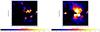 |
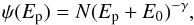
Fig. 1 Residual map for the “standard” diffuse background model with (left panel) and without (right panel) subtraction of the contribution from the weak unassociated 3FGL catalogue sources. |
Fitting results for different models.
2. Data analysis
We selected observations with Fermi-LAT of the regions towards the GC over the period that covers 5.5 yrs of exposure time (MET 239557417 – MET 415533077). For the data reduction, we used the standard Fermi-LAT analysis software package v9r33p01. In the analysis we selected all γ-ray events with energies exceeding 100 MeV. The region of interest (ROI) was defined to be a 10° × 10° square centred on the position of GC. To reduce the effect of the background related to the Earth albedo, we excluded the time intervals when the Earth was in the field of view from the analysis (more specifically, when the centre of the field of view was 52° above the zenith), as well as the time intervals when parts of the ROI were observed at zenith angles > 100°.
The spectral analysis was performed based on the P7rep_v15 version of the post-launch instrument response functions (IRFs). Both the front and back converted photons were selected. Since the Galactic diffuse model provided by the Fermi collaboration2 already contains some anomalous excess in the GC region, we did not use it to account for the Galactic diffuse background. Instead, we used an old version of the Galactic diffuse background gal_2yearp7v6_v0.fit as suggested by Daylan et al. (2016). Alternatively, we also used a diffuse background model based on the Planck opacity map (Planck Collaboration IX 2011). It is assumed that the dust opacity map exactly traces the column density and a constant cosmic ray (CR) distribution in ROI. In this regard we note that the Galprop code (Vladimirov et al. 2011) predicts a 20 percent or less gradient of the CR distribution in this compact region. Then the diffuse γ-ray emission produced by neutral pion decay and the electron bremsstrahlung becomes proportional to the gas column density and the dust opacity. We also included the inverse Compton (IC) component of the background using the Galprop code3, for the CR electrons distributions and the interstellar radiation fields (ISRF). Finally, the isotropic templates (iso_source_v05.txt) related to the CR contamination and the extragalactic γ-ray background were also included in the analysis.
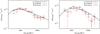 |
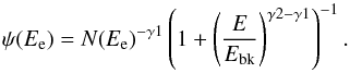
Fig. 2 Spectral energy distributions of γ-rays obtained for the northern (left panel) and southern (right panel) extended residual templates. The points with error bars are derived from the fitting procedure with (black symbols) and without (red symbols) subtracting the contribution from the unassociated 3FGL catalogue sources. The curves represent the best spectral fits for the hadronic (π0 – decay) channel (for details see the text). |
To take point-like sources into account that appear within ROI, we used the 3FGL source catalogue (Acero et al. 2015). In the likelihood analysis, the flux of point sources inside the ROI and all diffuse spatial templates are left as free parameters.
2.1. Morphological analysis
For morphological studies, we use only high energy (above 1 GeV) events as a first step. We fit the data with the catalogue sources, applying both the standard diffuse background model (gal_2yearp7v6_v0.fit + iso_source_v05.txt ) and the new diffuse background model (dust opacity map + galprop IC map +iso_source_v05.txt) with or without additional NFW template (see e.g. Daylan et al. 2016). The fitting results are summarized in Table 1. The TS value for the extended structure is defined as TS = −2Log(LNFW/Lnull, where LNFW and Lnull are the likelihood function values for the model with and without the NFW template. The results show that the additional NFW template indeed significantly improves the fitting procedure for both diffuse background models. Thus, our results confirm the conclusions of previous studies (e.g. Daylan et al. 2016; Macias & Gordon 2014). This is not a surprise given that the basic assumptions in ours and the previous studies are very similar, except for including the 3FGL source catalogue in our study. However, this cannot be used as an argument in favour of a dark matter origin of the “excess” radiation.
However, the improvement in the signal after applying the NFW template cannot be interpreted as a support of the dark matter origin of the “excess” radiation. In fact, it is not obvious that the GeV excess has the same spherical symmetric morphology as the a priori chosen NFW template.
To pursue this issue, in Fig. 1 we show the residual maps for fittings with the “standard” diffuse background model without the NFW template. Indeed, the residual maps reveal significant excess to the northern and southern regions, while there is no excess inside the plane. This motivates us to investigate the impact of the “bipolar” morphology on the the excess radiation. Furthermore, the 3FGL catalogue includes many unassociated point sources near the GC. To investigate alternative possibilities, such as assuming that these unassociated sources are a part of some extended structures, we omitted them when producing the residual map. The result is shown in Fig. 1. To test this hypothesis further, we derived spatial templates based on the residual maps without the unassociated sources and used it in the likelihood fitting instead of the NFW template. The relevant estimates of the statistical significance are presented in Table 1.
The removal of the contamination caused by the diffuse emission from the Galactic plane is an important part of the procedure of extraction of the new component of radiations. The current limited understanding of both the gas and CR distributions does not allow us to exclude the possibility that the bipolar structure is a result of subtraction of an overestimated contribution from the Galactic plane. On the other hand, it is not easy to produce a spherical symmetric residual from the data. This means that it would require a quite specific template, which significantly deviates from any conventional template used in the literature. This is also confirmed by the likelihood fitting. For both diffuse background models, the bipolar residual templates reveal a significantly larger likelihood ratio compared to the spherical templates: 882 (29σ) versus 544 (23σ) in the standard model and 1110 (33σ) versus 602 (24σ) in the new diffuse model (see Table.1). Furthermore, The Fermi-LAT Collaboration (2015) describe the latest Fermi official results for this region, which also show biconical residuals in the same region by using a carefully chosen Galactic diffuse background model. Thus we may conclude that the residual template with a bipolar structure correctly represents the spatial morphology of the GeV excess. In next section we use the standard diffuse model and the residual template as our fiducial model to derive the spectral information about the new component of the γ-ray emission.
2.2. Spectral analysis
To find the SED of the excess, we divided the entire energy range 300 MeV−30 GeV into eleven logarithmically equal energy intervals and applied the gtlike tool to each of these intervals. The results are shown in Fig. 2. All data points have test statistic (TS) values greater than 4, which corresponds to a statistical significance of more than 2σ. The spectra of both the northern and southern regions show maximum of SED at about 2 GeV, but above 2 GeV the spectrum of the northern part is slightly harder than that of the southern part ( 2.4 ± 0.1 versus 2.7 ± 0.1). To test the possible difference between the energy spectral of these two parts further, we tried to fit both SED above 2 GeV with the same power law index but with different absolute fluxes. This procedure gives χ2/d.o.f. = 14/9, which corresponds to a p value of 0.12. Thus the hypothesis that the two parts have the same spectral shape is rejected at the level of 1.5σ. The different spectra of the northern and southern parts would be an independent argument against the interpretation of the gamma-ray fluxes by dark matter, but for the available data set, the evidence is only marginal. Finally, it should be noted that at low energies, the spectra of the northern and southern components are softer than the spectrum derived when the NFW template is used. In Fig. 2 we show the results from the likelihood fitting with and without unassociated point sources. The difference between the two cases does not exceed 10% in any energy range for the northern part. However, for the first energy bin of the spectrum of the southern part, the difference is significantly larger. As a result, the photon index below the peak in the spectrum of the southern part ranges between 0.5 and 2.
To compare our results with the results reported by other groups, we performed a likelihood fitting by using the NFW profile (see, e.g., Daylan et al. 2016) and 2FGL catalog. The results are shown in Fig. 3. The derived SED peaks at about 2 GeV, and shows a very hard spectrum below the peak which is consistent with the spectra reported e.g. by Daylan et al. (2016) and Macias & Gordon (2014). This consistency implies that the difference in the spectra arising from the bipolar template, is a real effect, but not a result of biases in the analysis.
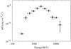 |
Fig. 3 Spectral energy distribution of γ-rays obtained for the NFW templates. |
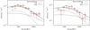 |
Fig. 4 Best fit spectra of leptonic γ-rays for the northern (left panel) and southern (right panel) parts of the excess. The red and black data points are the same as in Fig. 2. The dotted curves represent the contribution from bremsstrahlung, the dot-dashed line represent ICs, and the solid curves are the summations. |
3. Radiation mechanism
Based on the claimed distinct spectral shape of the GeV excess emission, the dark matter origin of that emission has been intensively discussed in recent years (Goodenough & Hooper 2009; Abazajian & Kaplinghat 2012; Daylan et al. 2016; Macias & Gordon 2014; Calore et al. 2015; Lacroix et al. 2014) as an exciting, although not a unique scenario (e.g., Carlson & Profumo 2014; Macias et al. 2015; Petrović et al. 2014; Cholis et al. 2015; Abazajian et al. 2015; Huang et al. 2015). Our independent analysis of the Fermi-LAT data confirms there is a new low energy γ-ray component, but not the previously reported spectral shape of radiation. With the spatial templates adopted in our study, we found a smoother SED around 1 GeV that can be readily explained by interactions of the cosmic ray protons and/or electrons without invoking specific or non-standard assumptions. Remarkably, for the given radiation and gas densities, three radiation mechanisms could comparably contribute to the γ-ray production in this energy band: (i) interactions of protons and nuclei with the ambient gas through the production and decay of π0-mesons; (ii) electron bremsstrahlung; and (iii) IC scattering of electrons. The average gas column density for the central 10-degree region exceeds 1022 cm-2 (Planck Collaboration IX 2011). Assuming that it is mostly contributed by the gas from the central 1 kpc region, the average hydrogen number density in this region is estimated to be ~3 cm-3, which we then use as a fiducial value in further calculations of γ-ray production.
-
π0-decay gamma rays The results shown in Fig. 2, indicate an apparent softening of the γ-ray spectra with an increase in energy for both southern and northern parts of emission. This can be easily explained by assuming the proton spectrum in the following form
 (1)where Ep is the proton kinetic energy. We note that E0 = 1 GeV implies a power-law spectrum in total energy: E = Ep + mpc2. The results of gamma-ray calculations for the northern and southern parts are shown in Fig. 2. For the northern part, the best fit is achieved for E0 = 1 GeV and γ = 2.4, while for the southern part E0 = 5 GeV and γ = 2.7. The spectral change in the proton energy distribution around E0 in Eq. (1) can be for various reasons. In particular, it is possible that the CRs are accelerated in very dense regions where ionization losses, which dominate at low energies, make the spectrum harder (de Boer et al. 2015). Secondly, the gas distribution may be very clumpy and the low-energy CRs cannot penetrate the dense cores of these clumps because of slower diffusion (Zirakashvili & Aharonian 2010; Gabici & Aharonian 2014). Finally, such a spectral shape with a cutoff (or break) around a few GeV can be a result of a specific (e.g.) stochastic mechanism of particle acceleration.
 -
Leptonic origin of gamma rays Quite remarkably, a break at GeV energies is also required in the spectrum of electrons to explain the deficit in low-energy gamma rays within both the leptonic (bremsstrahlung and IC) channels. Interestingly, such a low-energy cutoff, does exist in the interstellar electron spectrum (Strong et al. 2011; Webber & Higbie 2013) as well. In particular, the electron spectrum derived from direct observations and from ratio data show an energy break at several GeV, with spectral indices 1.8 and 2.8 below and above Ebk, respectively. These measurements can described by the following expression:
 (2)For the fit we leave Ebk and N as free parameters.
Both bremsstrahlung and IC scattering can significantly contribute to the γ-ray production. The emissivity of IC depends on the energy density of the interstellar radiation fields (ISRF). Here we adopt the value provided by GALPROP, in which the energy density of ISRF drops from 18.8 eV/cm3 at a height z = 100 pc to 3.3 eV/cm3 at z = 1 kpc. With such ISRF and an average gas density of about 3 cm-3, the IC and bremsstrahlung channels give similar contributions to GeV γ-rays. Remarkably, the electrons of approximately same energy contribute to the production of 100 MeV to 10 GeV γ-rays through these two channels.
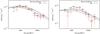 |
Fig. 5 Best fit spectra for the northern (left panel) and southern (right panel) parts of the excess by interactions of electrons through the electron bremsstrahlung (solid curves) and the IC channels (dotted curves). The red and black data points are the same as in Fig. 2. The curves for bremsstrahlung and ICs are normalized so as to explain the measurements separately (for details see the text). |
The results in Fig. 4 show that the observed γ-ray fluxes can be explained by a combination of contributions of these two channels. However, the gas density in this specific region contains non-negligible uncertainties. It can be higher or lower than the one adopted in Fig. 4. In that case the radiation would be dominated by the bremsstrahlung or IC channels, respectively. In either case, with a slight adjustment of the parameters of the electron spectrum and the normalization factor in Eq. (1), we can explain the γ-ray data. It is demonstrated in Fig. 5.
For both the bremsstrahlung and hadronic channels, the γ-ray emissivity is proportional to nCR × ngas, where nCR and ngas are the CR (electrons or protons) and the gas densities, respectively. The recent measurements of the Planck satellite provide the distribution of the gas column density throughout the Galaxy (Planck Collaboration IX 2011). Thus, using the information of the spatial distribution of the γ-ray flux, we can derive the spatial distributions of the CR density. For this reason, we divide the templates into slices with different latitudes (| b | = [ 1°,2° ] , [ 2°,3° ] and [ 3°,5° ] for both northern and southern parts ). For a better angular resolution we use data with energy of γ-rays exceeding 1 GeV. We also exclude the inner one-degree region from this analysis to prevent the contamination from the bright central source.
To derive the gas column density, we use the formula relating the dust opacity and the column density, using the dust as the reference emissivity according to Eq. (4) of the paper of Planck Collaboration IX (2011): ![Mathematical equation: \begin{equation} \label{eq:dust} \tau_{\rm M}(\lambda) = \left(\frac{\tau_{\rm D}(\lambda)}{N_{\rm H}}\right)^{\rm dust}[N_{{\rm H I}}+2X_{\rm CO}W_{\rm CO}], \end{equation}](/articles/aa/full_html/2016/05/aa27550-15/aa27550-15-eq47.png) (3)where τM is the dust opacity as a function of the wavelength λ, (τD/NH)dust is the reference dust emissivity measured in low-NH regions, WCO is the integrated brightness temperature of the CO emission, and XCO = NH2/WCO is the so-called H2/ CO conversion factor. Substituting the latter into Eq. (3), one obtains
(3)where τM is the dust opacity as a function of the wavelength λ, (τD/NH)dust is the reference dust emissivity measured in low-NH regions, WCO is the integrated brightness temperature of the CO emission, and XCO = NH2/WCO is the so-called H2/ CO conversion factor. Substituting the latter into Eq. (3), one obtains ![Mathematical equation: \begin{eqnarray} N_{\rm H} = N_{{\rm H I}} +2 N_{{\rm H}_2} = \tau_{\rm m}(\lambda)\left[\left(\frac{\tau_{\rm D}(\lambda)}{N_{\rm H}}\right)^{\rm dust}\right]^{-1}\cdot \end{eqnarray}](/articles/aa/full_html/2016/05/aa27550-15/aa27550-15-eq55.png) (4)We use a dust emissivity at 353 GHz of
(4)We use a dust emissivity at 353 GHz of  cm2, from Table 3 of Planck Collaboration IX (2011). Then, to find the γ-ray emissivities per H-atom, we divide the γ-ray flux by the column density. This value should be proportional to the CR density. The results for the southern part of the excess are summarized in Fig. 6. The results for northern part of the excess are similar. The spatial distribution of the CR density depends on the injection history. In the spherically symmetric case, assuming that the CR accelerator is located in the GC region, the impulsive injection predicts a constant distribution with the distance r, while the continuous injection predicts a profile 1 /r. Finally, if CR transportation proceeds via wind, it should have a 1 /r2 profile. All the profiles are indicated in Fig. 6. One can see that the radial distribution of the CR density derived from the spatial distributions of γ rays and the gas is best explained by an impulsive injection.
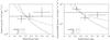 |
Fig. 6 Radial profiles of the γ-ray emissivity for the southern parts of the excess. For comparison, we show the constant (solid curves), 1 /r (dotted curves), and 1 /r2 (dot-dashed curves) profiles, which are predicted by the impulsive injection, continuous injection, and the transport through wind, respectively. Left panel: emissivity per hydrogen atom related to interactions with gas (i.e. inelastic interactions of protons and ions or bremsstrahlung of electrons). Right panel: γ-ray emissivity due to IC normalized to the density of ISRF 1 eV/cm3. |
In the IC scenario, the γ-ray emissivity is normalized to 1 eV/cm3 energy density of ISRF. To derive the radial distribution of this quantity, we divided the gamma-ray flux by the ISRF density in each slice as described above. The results are shown in Fig. 6. In this case, a radial dependence of the CR electron distribution closer to 1/r type profile is explained by the fact that the distribution of ISRF is more homogeneous than the gas distribution. We should mention the work of Petrović et al. (2014) and Cholis et al. (2015), who claim that the excess of the radiation could be mainly contributed by the IC scattering of electrons. However, the results in Figs. 2, 4, and 5 demonstrate that at this stage we cannot give a preference to any of three alternatives related to the pp, the electron bremsstrahlung and IC scenarios.
Thus while the interpretation of the morphology of γ-rays within the pp and the electron bremsstrahlung scenarios demands a burst type injection, the interpretation of data within the IC scenario gives a preference to the continuous injection. Apparently, the question of the injection regime should be specified by the timescale of formation of these large structures. If the particle propagation is dominated by diffusion, the characteristic timescale is t ~ R2/ 6D ~ 106 to 107 yrs, depending on the diffusion coefficient D of CRs at GeV energies.
Another important concern for understanding the origin of these particles is the total energy budget. The total luminosity of both the northern and southern parts is about 1037 erg/s. Then, the required CR energy budget for a hadronic scenario is 1052(3 cm-3/ n) erg. For the leptonic scenarios, the energetics are somewhat (factor of 5 and 3) less for the electron bremsstrahlung and IC channels, respectively. All these estimates exceed the typical CR energy release in a single supernova explosion by 1.5 to 2 orders of magnitude.
If the GeV excess is dominated by interactions of protons or electrons with the ambient gas, so that an impulsive injection is preferred, the required energy release in these low-energy CRs can be related to the higher activity of the GC in the past, some 106−7 yrs ago. This agrees with the conclusion based on the recent studies of the Hα emission in the so-called Magellanic stream (Bland-Hawthorn et al. 2013). On the other hand, the IC scenario prefers a (quasi) constant injection, so the GeV electrons can be linked to other source populations, in particular to supernova remnants, stellar clusters, pulser wind nebulae, binary systems, etc.
4. Conclusions
We performed a new analysis based on the 5.5-yrs of observations of Fermi-LAT in the 10° × 10° region towards the GC with a focus on the so-called GeV excess reported previously. We found that the morphology of this extra component of γ-rays would prefer a bipolar to a spherically symmetric structure. Moreover, the γ-ray energy spectra appear smoother than reported in the previous studies. We argued that the energy spectra can be fitted by both hadronic and leptonic channels of γ-ray production. In the case of leptonic origin of this radiation component, the contributions from interactions of electrons with the ambient gas and radiation fields are comparable. But the dominance of either the electron bremsstrahlung or the IC scattering cannot be excluded given the uncertainties of the gas density in the production region. The total energy budget in a parent’s charged particles in the leptonic scenarios is less, by a factor of a few, than in protons. The estimates exceed the CR energy that can be provided by a single SNR by 1.5 to 2 orders of magnitudes.
Alternatively, these particles can be related to other source populations, in particular to pulsars (or pulsar wind nebulae), to the relativistic jets of binary systems, to powerful stellar winds in compact stellar clusters, and of course, to Sgr A*, the central supermassive black hole in the GC. Both the hadronic and the electron bremsstrahlung scenarios lean towards a burst type injection of particles (over the last 106−7 yrs), which would favour a possible link of these particles to a high activity of Sgr A*, On the other hand, the IC scenario, which favours a continuous injection, is not excluded. To distinguish between these
possibilities we need a comprehensive modelling of the propagation and radiation of GeV protons and electrons in the central several kpc region of the inner Galaxy. Such studies can provide important insight into the origin of the GeV excess and its relation to other CR accelerators in that most active part of our Galaxy.
gll_iem_v05_rev1.fit, available at http://fermi.gsfc.nasa.gov/ssc/data/access/lat/BackgroundModels.html
References
- Abazajian, K. N., & Kaplinghat, M. 2012, Phys. Rev. D, 86, 083511 [NASA ADS] [CrossRef] [Google Scholar]
- Abazajian, K. N., Canac, N., Horiuchi, S., Kaplinghat, M., & Kwa, A. 2015, J. Cosmol. Astropart. Phys., 7, 13 [NASA ADS] [CrossRef] [Google Scholar]
- Acero, F., Ackermann, M., Ajello, M., et al. 2015, ApJS, 218, 23 [Google Scholar]
- Bartels, R., Krishnamurthy, S., & Weniger, C. 2016, Phys. Rev. Lett., 116, 051102 [NASA ADS] [CrossRef] [PubMed] [Google Scholar]
- Bland-Hawthorn, J., Maloney, P. R., Sutherland, R. S., & Madsen, G. J. 2013, ApJ, 778, 58 [NASA ADS] [CrossRef] [Google Scholar]
- Calore, F., Cholis, I., & Weniger, C. 2015, J. Cosmol. Astropart. Phys., 3, 38 [Google Scholar]
- Carlson, E., & Profumo, S. 2014, Phys. Rev. D, 90, 023015 [NASA ADS] [CrossRef] [Google Scholar]
- Cholis, I., Evoli, C., Calore, F., et al. 2015, JCAP, 12, 005 [NASA ADS] [CrossRef] [Google Scholar]
- Daylan, T., Finkbeiner, D. P., Hooper, D., et al. 2016, Phys. Dark Universe, 12, 1 [Google Scholar]
- de Boer, W., Gebauer, I., Kunz, S., & Neumann, A. 2015, ArXiv e-prints [arXiv:1509.05310] [Google Scholar]
- Gabici, S., & Aharonian, F. A. 2014, MNRAS, 445, L70 [NASA ADS] [CrossRef] [Google Scholar]
- Goodenough, L., & Hooper, D. 2009, ArXiv e-prints [arXiv:0910.2998] [Google Scholar]
- Huang, X., Enßlin, T., & Selig, M. 2015, ArXiv e-prints [arXiv:1511.02621] [Google Scholar]
- Lacroix, T., BÅ‘hm, C., & Silk, J. 2014, Phys. Rev. D, 90, 043508 [NASA ADS] [CrossRef] [Google Scholar]
- Macias, O., & Gordon, C. 2014, Phys. Rev. D, 89, 063515 [NASA ADS] [CrossRef] [Google Scholar]
- Macias, O., Gordon, C., Crocker, R., & Profumo, S. 2015, MNRAS, 451, 1833 [NASA ADS] [CrossRef] [Google Scholar]
- Mirabal, N. 2013, MNRAS, 436, 2461 [NASA ADS] [CrossRef] [Google Scholar]
- Petrović, J., Dario Serpico, P., & Zaharijaš, G. 2014, J. Cosmol. Astropart. Phys., 10, 52 [NASA ADS] [CrossRef] [Google Scholar]
- Planck Collaboration IX. 2011, A&A, 536, A19 [NASA ADS] [CrossRef] [EDP Sciences] [Google Scholar]
- Strong, A. W., Orlando, E., & Jaffe, T. R. 2011, A&A, 534, A54 [NASA ADS] [CrossRef] [EDP Sciences] [Google Scholar]
- The Fermi-LAT Collaboration 2015, ArXiv e-prints [arXiv:1511.02938] [Google Scholar]
- Vladimirov, A. E., Digel, S. W., Jóhannesson, G., et al. 2011, Comput. Phys. Comm., 182, 1156 [Google Scholar]
- Webber, W. R., & Higbie, P. R. 2013, ArXiv e-prints [arXiv:1308.6598] [Google Scholar]
- Yuan, Q., & Zhang, B. 2014, J. High Energy Astrophysics, 3, 1 [NASA ADS] [CrossRef] [Google Scholar]
- Zhou, B., Liang, Y.-F., Huang, X., et al. 2015, Phys. Rev. D, 91, 123010 [NASA ADS] [CrossRef] [Google Scholar]
- Zirakashvili, V. N., & Aharonian, F. A. 2010, ApJ, 708, 965 [NASA ADS] [CrossRef] [Google Scholar]
All Tables
All Figures
|
Fig. 1 Residual map for the “standard” diffuse background model with (left panel) and without (right panel) subtraction of the contribution from the weak unassociated 3FGL catalogue sources. |
| In the text | |
|
Fig. 2 Spectral energy distributions of γ-rays obtained for the northern (left panel) and southern (right panel) extended residual templates. The points with error bars are derived from the fitting procedure with (black symbols) and without (red symbols) subtracting the contribution from the unassociated 3FGL catalogue sources. The curves represent the best spectral fits for the hadronic (π0 – decay) channel (for details see the text). |
| In the text | |
|
Fig. 3 Spectral energy distribution of γ-rays obtained for the NFW templates. |
| In the text | |
|
Fig. 4 Best fit spectra of leptonic γ-rays for the northern (left panel) and southern (right panel) parts of the excess. The red and black data points are the same as in Fig. 2. The dotted curves represent the contribution from bremsstrahlung, the dot-dashed line represent ICs, and the solid curves are the summations. |
| In the text | |
|
Fig. 5 Best fit spectra for the northern (left panel) and southern (right panel) parts of the excess by interactions of electrons through the electron bremsstrahlung (solid curves) and the IC channels (dotted curves). The red and black data points are the same as in Fig. 2. The curves for bremsstrahlung and ICs are normalized so as to explain the measurements separately (for details see the text). |
| In the text | |
|
Fig. 6 Radial profiles of the γ-ray emissivity for the southern parts of the excess. For comparison, we show the constant (solid curves), 1 /r (dotted curves), and 1 /r2 (dot-dashed curves) profiles, which are predicted by the impulsive injection, continuous injection, and the transport through wind, respectively. Left panel: emissivity per hydrogen atom related to interactions with gas (i.e. inelastic interactions of protons and ions or bremsstrahlung of electrons). Right panel: γ-ray emissivity due to IC normalized to the density of ISRF 1 eV/cm3. |
| In the text | |
Current usage metrics show cumulative count of Article Views (full-text article views including HTML views, PDF and ePub downloads, according to the available data) and Abstracts Views on Vision4Press platform.
Data correspond to usage on the plateform after 2015. The current usage metrics is available 48-96 hours after online publication and is updated daily on week days.
Initial download of the metrics may take a while.