| Issue |
A&A
Volume 589, May 2016
|
|
|---|---|---|
| Article Number | A25 | |
| Number of page(s) | 18 | |
| Section | Planets and planetary systems | |
| DOI | https://doi.org/10.1051/0004-6361/201527522 | |
| Published online | 07 April 2016 | |
The HARPS search for southern extra-solar planets
XL. Searching for Neptunes around metal-poor stars⋆
1
Instituto de Astrofísica e Ciências do Espaço, Universidade do
Porto, CAUP, Rua das
Estrelas, 4150-762
Porto,
Portugal
e-mail:
This email address is being protected from spambots. You need JavaScript enabled to view it.
2
Departamento de Física e Astronomia, Faculdade de Ciências,
Universidade do Porto, Rua Campo
Alegre, 4169-007
Porto,
Portugal
3
SUPA, School of Physics and Astronomy, University of St
Andrews, St Andrews
KY16 9SS,
UK
4
Harvard-Smithsonian Center for Astrophysics, 60 Garden
Street, Cambridge,
MA
02138,
USA
5
Aix Marseille Université, CNRS, LAM (Laboratoire d’Astrophysique
de Marseille) UMR 7326, 13388
Marseille,
France
6
European Southern Observatory, Casilla 19001, Santiago, Chile
7
Observatoire de Genève, Université de Genève,
51 chemin des Maillettes,
1290
Sauverny,
Switzerland
8
Cavendish Laboratory, J J Thomson Avenue, Cambridge, CB3 0HE, UK
9
INAF–Osservatorio Astrofisico di Torino, via Osservatorio
20, 10025
Pino Torinese,
Italy
Received: 7 October 2015
Accepted: 4 January 2016
Abstract
Context. As a probe of the metallicity of proto-planetary disks, stellar metallicity is an important ingredient for giant planet formation, most likely through its effect on the timescales in which rocky or icy planet cores can form. Giant planets have been found to be more frequent around metal-rich stars, in agreement with predictions based on the core-accretion theory. In the metal-poor regime, however, the frequency of planets, especially low-mass planets, and the way it depends on metallicity are still largely unknown.
Aims. As part of a planet search programme focused on metal-poor stars, we study the targets from this survey that were observed with HARPS on more than 75 nights. The main goals are to assess the presence of low-mass planets and provide a first estimate of the frequency of Neptunes and super-Earths around metal-poor stars.
Methods. We performed a systematic search for planetary companions, both by analysing the periodograms of the radial-velocities and by comparing, in a statistically meaningful way, models with an increasing number of Keplerians.
Results. A first constraint on the frequency of planets in our metal-poor sample is calculated considering the previous detection (in our sample) of a Neptune-sized planet around HD 175607 and one candidate planet (with an orbital period of 68.42 d and minimum mass Mpsini = 11.14 ± 2.47 M⊕) for HD 87838, announced in the present study. This frequency is determined to be close to 13% and is compared with results for solar-metallicity stars.
Key words: methods: data analysis / planetary systems / surveys / stars: individual: HD 87838 / techniques: radial velocities
Based on observations collected at ESO facilities under programs 082.C-0212, 085.C-0063, 086.C-0284, and 190.C-0027 (with the HARPS spectrograph at the ESO 3.6-m telescope, La Silla-Paranal Observatory).
© ESO, 2016
1. Introduction
More than 600 exoplanets were discovered and many others confirmed using radial-velocity (RV) observations (www.exoplanet.eu, Schneider et al. 2011). The method is more sensitive to massive planets orbiting close to their stars, since Neptune- and Earth-mass planets induce very small amplitude radial-velocity signals, often at the level of the current observational uncertainties of 1 ms-1 and weaker. In addition, stellar activity can induce false-positive signals that mimic and mask the radial velocity signature of a low-mass planet (e.g. Bonfils et al. 2007; Robertson & Mahadevan 2014; Santos et al. 2014). Only with very high precision Doppler spectroscopy and dense sampling is one able to detect these planets (e.g. Dumusque et al. 2012; Hatzes 2014) and to push the detection limits in the direction of a possibly habitable Earth-like planet, the same stars must be followed for a very long time.
The increasing number of detected planets provides constraints for models of planet formation and evolution (e.g. Udry & Santos 2007; Ida & Lin 2004; Mordasini et al. 2009). In particular, the metallicity and, in general, the chemical abundances of the host star, are now known to be a key ingredient in planet formation (Ida & Lin 2004; Mordasini et al. 2015). According to the core-accretion theory, proto-planetary disks with higher metallicity are able to form rocky or icy cores in time for runaway accretion to lead to the formation of a giant planet before disk dissipation occurs. In lower metallicity disks, the cores do not grow fast enough to accrete gas in large quantities before disk dissipation occurs, implying a lower fraction of giant planets.
Stellar parameters for each of the 15 stars studied here.
Gonzalez (1997) showed the first observational hints for a correlation between the presence of giant planets and metallicity. As more and more planets were discovered, this correlation was solidly confirmed: it is more likely to detect a giant planet orbiting a metal-rich star (Santos et al. 2004; Fischer & Valenti 2005; Sousa et al. 2011b). This result was also confirmed in data from transit surveys (e.g. Buchhave et al. 2012). Furthermore, it is also now known that the metallicity, or even specific chemical abundance ratios, can have a strong impact on the planet formation efficiency, composition, and architecture (Guillot et al. 2006; Adibekyan et al. 2013, 2015; Dawson et al. 2015; Santos et al. 2015).
Because giant planets are more frequent around metal-rich stars, several RV surveys became biased towards metal-rich samples (Tinney et al. 2002; Fischer & Valenti 2005; Melo et al. 2007; Jenkins et al. 2013a). Nevertheless, some programmes focused on the metal-poor regime and tried to determine the frequency of giant planets orbiting metal-poor stars and the metallicity limit below which no giant planets can be observed (Sozzetti et al. 2009; Santos et al. 2011; Mortier et al. 2012, 2013). Until recently, however, these programmes focused on the search for massive, giant planets.
Neptune-mass planets, in contrast, have been found to have a relatively flat metallicity distribution (Udry et al. 2006; Sousa et al. 2008, 2011b; Neves et al. 2013). In systems with only hot Neptunes, the metallicity distribution actually becomes slightly metal-poor (Mayor et al. 2011; Buchhave et al. 2012). These results are supported by theoretical models that predict lower mass planets are common around stars with a wide range of metallicities. One should note here the works of Wang & Fischer (2014) and Buchhave & Latham (2015), who find conflicting results about the existence of a universal planet-metallicity correlation extending to the terrestrial planets, and Adibekyan et al. (2012), who show that, in the metal-poor regime, planets are more prevalent on α-enhanced stars (i.e. of higher global metallicity).
The number of detected low-mass planets orbiting metal-poor stars is nevertheless still small. In an effort to detect these planets and explore the low-metallicity regime, our team started a Large Programme with HARPS to follow a sample of about 100 metal-poor stars. The programme and sample were presented in Santos et al. (2014), to which we point the reader for more details. The main goal of the survey is to derive observational constraints on the frequency of Neptunes and super-Earths in the metal-poor regime. These estimates will be compared with the ones from the HARPS-GTO programme (Mayor et al. 2011), which searched for very low-mass planets orbiting a sample of solar-neighbourhood stars (thus with solar metallicities). When combined, the two surveys will set important constraints for planet formation and evolution models and help in providing an estimate of the frequency of planets in our Galaxy.
This paper presents the analysis of the stars in the metal-poor sample that were observed on more than 75 nights. Some of these stars now have precise radial velocity observations covering a baseline of over ten years. In Sect. 2 we present the stellar parameters for these stars and their radial-velocity observations. The method used to search for Keplerian signals is outlined in Sect. 3 and in Sect. 4 the results of its application. Section 5 presents a simple comparison of the model selection criteria we consider, and detection limits for individual stars are derived in Sect. 6. A first constraint on the occurrence of planets in this sample and our conclusions are presented in Sect. 7.
2. Sample and observations
Our complete sample of metal-poor stars contains 109 targets, chosen from a survey for giant planets orbiting metal-poor stars (Santos et al. 2007), and a programme to search for giant planets orbiting a volume-limited sample of FGK dwarfs (Naef et al. 2007). The criteria for defining this sample are detailed in Santos et al. (2014). Stellar parameters were derived for the complete sample from a set of high-resolution HARPS spectra (Sousa et al. 2011a; Santos et al. 2014).
In this work we analyse those stars that, up to December 2014, were observed on more than 75 nights. Though not strictly motivated, this number of nights means that in the worst case scenario, we have six data points per parameter for a model with two planets. A total of 15 stars meet this criterion. In Table 1 we present the stellar parameters for this subsample. The table lists the stellar mass, effective temperature, surface gravity, metallicity, B − V colour, activity level, and estimated rotation period.
The activity level of the stars, denoted here by the weighted average of the  values (Noyes et al. 1984b), was derived from the analysis of the CaII H and K lines in the HARPS spectra (e.g. Santos et al. 2000; Lovis et al. 2011). Estimates for the rotation period of each star were derived from the activity-rotation calibrations of Noyes et al. (1984b) and Mamajek & Hillenbrand (2008). The typical error bar on these estimates, computed from the dispersion in the time series, is close to the difference between the estimates from the two calibrations. For HD 31128, the rotation period derived in this way is around 2.8 d. The very low metallicity of this star, however, places it outside the calibration range of the flux calibration and of the adopted activity-rotation relations. This renders the rotation period estimate uncertain, so we chose to omit it from the table.
Table 2 shows the number of nights each star was observed, the mean error bar  , and the weighted standard deviation of the radial velocities sRV. The ratio of the last two quantities gives an indication of whether the radial-velocities vary in excess of the internal errors and by how much. This table also shows the baseline of observations.
The distributions of metallicity, effective temperature, and surface gravity of the full sample and of the 15 stars studied here are shown in Fig. 1. By selecting stars based on the number of observations, one can introduce biases that depend on the criteria used for scheduling observations. From the distributions in Fig. 1, we do not see a clear bias towards warmer or more evolved stars, which may show more significant (stellar) variability. The subsample can nevertheless be biased in favour of stars hosting low-mass planets, since these stars will also show more significant variability. This can have an impact on our determination of the planet frequency (Sect. 7), although it is difficult to determine to what extent. Regarding metallicity, the subsample is representative of the overall distribution but does not cover the complete metallicity range.
Number of individual night observations, average RV errorbar, weighted standard deviation of the RV measurements, and timespan for each of the targets.
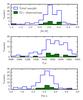 |
Fig. 1 Metallicity, effective temperature, and surface gravity distributions for the full metal-poor sample (blue histograms) and the 15 stars observed on more than 75 different nights (green filled histograms). |
For these 15 stars, we analyse a total of 1540 radial velocity measurements obtained using the HARPS spectrograph at the 3.6 m ESO telescope (La Silla-Paranal Observatory). All observations were reduced with the HARPS pipeline (version 3.5), where the radial velocities were obtained by performing a cross-correlation of the observed spectrum with a numerical mask (Baranne et al. 1996; Pepe et al. 2002).
For the first measurements (obtained before the present Large Programme and still within the HARPS GTO programme), the exposure times were not long enough to average out the noise coming from stellar oscillations, and the radial velocities had a limiting precision of around 2 ms-1. The observing strategy was revised later by setting exposure times to 900 s, resulting in a precision of the order of 1 ms-1. With the start of the Large Programme, in October 2012, we aimed at obtaining more than one spectrum of the star in a given night, separated by several hours.
We use nightly binned data in our analysis, thus focusing on signals with periods longer than one night. The objective of this strategy is to minimize the impact of granulation phenomena on the radial velocities and improve the planetary detection limits (see Dumusque et al. 2011c). We note, however, that this observing strategy has some caveats since it has been designed for and tested in stars with solar metallicities, and its optimality is not guaranteed for metal-poor stars. Also, considering the binned data means we cannot assess the presence of shorter period planets (e.g. Dawson & Fabrycky 2010; Hatzes 2014; Grunblatt et al. 2015).
3. Methodology
As a first step in the analysis of each star, and as is standard when searching for planets in RV data, we computed the generalised Lomb-Scargle (GLS) periodogram (Zechmeister & Kürster 2009) of the radial velocities and searched for significant peaks. The significance of a peak is evaluated by the false alarm probability (FAP) estimated with a bootstrap permutation procedure, first devised by Murdoch et al. (1993; see also Endl et al. (2001), Mortier et al. (2012). The RV measurements and errorbars are (together) randomly redistributed with repetition, keeping the time stamps of observations fixed. For each randomization, a new GLS periodogram is computed, and its maximum power is compared with the original periodogram, thus obtaining the FAP levels. After repeating this process 1000 times, we show the estimated 1% and 0.1% FAP levels.
If any periodogram peak is deemed significant, we proceed with the analysis of the RV data together with other activity proxies to try to determine the nature of the signal. We focus on the FWHM of the HARPS cross-correlation function (CCF) and the proxy as the most reliable indicators of activity, even though we have also analysed other indicators. It may also be that a signal is present in the data that was created by a planet with a moderately high eccentricity. The standard GLS periodogram (which searches for sinusoidal signals) is then not the best tool for recovering it. Therefore, for the stars in which the periodogram does not show significant peaks, we still run a planet detection algorithm that compares the evidence for models with 0, 1, and 2 Keplerian signals (see below). For some stars that show evidence of a Keplerian signal, we try to assert its nature further.
As is now ubiquitous in the literature, our model for the radial-velocity observations vi is described by a Gaussian sampling distribution  (1)where Mn represents a model with n planets, V0 is a constant offset, Vn (ti,θ) is the radial-velocity shift caused by n orbiting planets, which depends on time ti and the planets’ orbital parameters θ. The parameter s is an extra “jitter” term, added in quadrature to the total measurement uncertainties σi, which allows for additional white noise to be taken into account.
We assume each planet induces a Keplerian signal k (t), such that Vn (t) = ∑ nk (t). This signal depends on the orbital period P, semi-amplitude K, eccentricity e, argument of the periastron ω, and time of periastron passage T0 (e.g. Perryman 2014, Chap. 2). When n = 0, we have Vn = 0 by definition.
To infer the number of Keplerians supported by a dataset d = { ti,vi,σi,i = 1,...,N } , we can calculate the marginal likelihood, or evidence En, for each of the models Mn: ![Mathematical equation: \begin{eqnarray} \label{eq:evidence} E_n = \p[{d} | M_n] = \int_\Theta \p[{d} | \Theta, M_n] \p[\Theta | M_n] {\rm d}\Theta, \end{eqnarray}](/articles/aa/full_html/2016/05/aa27522-15/aa27522-15-eq38.png) (2)where p(d | Θ,Mn) is the likelihood function and p(Θ | Mn) the prior distribution for the parameters of the model. Here, Θ has different dimensions, depending on the value of n and corresponds to the full set of parameters to be marginalised over, Θ = { V0,s,θ }. The likelihood is given by the product of the terms in Eq. (1)for each data point,
(2)where p(d | Θ,Mn) is the likelihood function and p(Θ | Mn) the prior distribution for the parameters of the model. Here, Θ has different dimensions, depending on the value of n and corresponds to the full set of parameters to be marginalised over, Θ = { V0,s,θ }. The likelihood is given by the product of the terms in Eq. (1)for each data point, ![Mathematical equation: \begin{eqnarray} \p[d | \Theta, M_n] &=& \left(2\pi\right)^{-N/2} \left[ \prod_{i\,=\,1}^N \left(\sigma_i^2 + s^2\right)^{-1/2} \right] \nonumber \\ && \quad \times \exp \left \{ - \sum_{i\,=\,1}^N \frac{\left[ v_i - V_0 - V_n\,(t_i, \theta) \right]^2}{2\left(\sigma_i^2 + s^2\right)} \right\}\cdot \end{eqnarray}](/articles/aa/full_html/2016/05/aa27522-15/aa27522-15-eq43.png) (3)The comparison between any pair of models is made by evaluating the associated odds ratio (e.g. Gregory 2010)
(3)The comparison between any pair of models is made by evaluating the associated odds ratio (e.g. Gregory 2010) ![Mathematical equation: \begin{eqnarray} \label{eq:odds} \mathcal{O}_{ij} = \frac{\p[M_i | {d}]}{p\,(M_j | {d})} = \frac{\p[M_i]}{p\,(M_j)} \cdot \frac{\p[{d} | M_i]}{p\,(d | M_j)} , \end{eqnarray}](/articles/aa/full_html/2016/05/aa27522-15/aa27522-15-eq44.png) (4)which simplifies to the ratio of the evidence when there is no prior preference for any model, that is, when
(4)which simplifies to the ratio of the evidence when there is no prior preference for any model, that is, when  . If there is a preference for a given model, it can be included directly in Eq. (4). In this work we chose to consider all models equally probable a priori. Kass & Raftery (1995) provide a qualitative scale for interpretating evidence ratio values.
To evaluate the difficult (multidimensional) integral in Eq. (2), we use the nested sampling algorithm (Skilling 2004) implemented in MultiNest (Feroz et al. 2009, 2013). The key idea in nested sampling is to update a set of points, originally sampled from the prior, with new samples that are subject to a hard likelihood constraint. At each iteration, the algorithm progressively moves towards regions of higher likelihood. Each time a new sample is obtained, it is assigned a value X ∈ [ 0,1 ] representing the amount of prior mass estimated to lie at a higher likelihood than that of the discarded point1. These X values introduce a mapping from the parameter space to the interval [ 0,1 ] or, in other words, they divide the prior volume into a large number of points with equal prior mass. In the new space, the prior becomes a uniform distribution, and the likelihood is a decreasing function of X. Then, the evidence can be computed by simple quadrature. For further details, the reader is referred to Skilling (2004), Mukherjee et al. (2006), Sivia & Skilling (2006), and Feroz et al. (2009).
Nested sampling also provides posterior samples for all parameters as a by-product. The necessary descriptive statistics can then be calculated from these samples. Estimating all the posterior distributions for a particular model is what we mean by fitting a Keplerian in the remainder of the paper. This algorithm has been tested and validated in the analysis of radial-velocity data by Feroz et al. (2011a,b) and Feroz & Hobson (2014).
Another way to approach the problem is to treat n (the number of Keplerians) itself as a free parameter of the model (so that it is part of Θ) and sample from its own posterior distribution, p(n | d), to infer the number of Keplerians present in the data. We use the recent algorithm proposed by Brewer & Donovan (2015) to sample from this distribution. The method uses trans-dimensional birth-death moves, within the context of diffusive nested sampling (Brewer et al. 2011), and it was found to give results comparable to MultiNest, often with a smaller number of likelihood evaluations and less computation time. The same likelihood function and priors were used for both methods.
We furthermore need to specify the priors for each of the parameters. It is through the priors that the Bayesian analysis can take the principle of parsimony and Occam’s razor into account. What is important is not (only) the number of parameters in a model but also the amount of support in their priors. This is the reason to choose uninformative and physically motivated priors.
The form and limits of the priors we use are shown in Table 3. A few of our choices merit further discussion. For the orbital periods, we use a Jeffrey’s prior between 1d and the timespan of each dataset. Apart from HD 56274 and HD 175607, which are analysed separately, none of the stars show clear long-term trends that could suggest the presence of long-period planets. We thus limit our search for periods that are shorter than the timespans, which are in fact very long already. The lower limit is due to our use of nightly binned observations. For the semi-amplitudes, a modified Jeffrey’s prior is used, spanning the range 0−10 ms-1 and with a “knee” at the mean error bar of each dataset. The choice of upper limit comes from the cuts used when defining the complete metal-poor sample (see Santos et al. 2014), which was stripped of stars showing large RV dispersions2. The same arguments apply to the jitter prior. The prior for the orbital eccentricities was suggested by Kipping (2013) after an analysis of the population of known exoplanets. Priors for the other parameters are uniform between what we consider to be sensible limits.
Model selection criteria other than the evidence can be more easily calculated using just the maximum-likelihood value  and the total number of parameters in the model, Npar. When presenting our results in Table 4, we include the values of the sample-corrected Akaike information criteria (AICC) and the Bayesian information criteria (BIC), calculated as described in Burnham & Anderson (2010):
  The preferred model when using these criteria is the one that gives the lowest AICC and BIC values. For the choice of one model to be significant one can require differences ΔAICC and ΔBIC around 10 (Burnham & Anderson 2010).
Priors for the model parameters.
4. Case-by-case results
In this section we present the individual analysis for each star. Plots with the radial-velocity data and GLS periodograms are shown in Figs. A.1–A.15, and a summary of the model-selection results for the stars without significant periodogram peaks is shown in Table 4.
4.1. Candidate planetary signals
HD 87838.
This star was observed 104 times on 87 different nights. The radial velocities show a dispersion of 2.4 ms-1 and a mean uncertainty of 1.3 ms-1. The GLS periodogram shows no significant peaks (Fig. A.1), but the Bayesian analysis finds slight evidence of one Keplerian signal (Table 4).
The strongest peaks in the periodogram are at 988 d, 68 d, and 334 d. The most convincing (highest likelihood) Keplerian fit is a signal with P = 68.34 ± 0.46 d, a semi-amplitude K = 1.9 ± 0.38 ms-1, and an eccentricity of 0.46 ± 0.16. If caused by a planet, this signal would correspond to a planet with a minimum mass of 11.14 ± 2.47 M⊕ at an orbital distance of 0.322 ± 0.001 AU. The phase-folded radial-velocities for this solution are shown in Fig. 2.
Analysing the and FWHM activity indicators, we do not find strong periodicities close to 68 d (Fig. 3), so it is unlikely that this signal is caused by stellar activity. (Indeed, the periodogram of the FWHM shows a non-significant peak close to the estimated rotation period.) Since the Bayesian analysis only gives marginal evidence of a Keplerian signal (a Bayes factor of 1.75 is “not worth more than a bare mention” in the scale of Kass & Raftery 1995), we consider that this detection is marginal and needs further confirmation. More data would certainly shed light on its true origin, and we will continue to observe this star in the future.
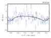 |
Fig. 2 Phase-folded RV curve for HD 87838 with a period of 68.42 d. The blue points indicate the measured radial-velocities, and red circles show the same radial velocities binned in phase with a bin size of 0.1. |
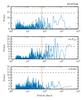 |
Fig. 3 Periodograms of the radial velocities (top) the |
HD 175607.
This star’s periodogram (Fig. A.2) shows a very significant peak at 29 d, coinciding almost exactly with the estimated rotation period (see Table 1). Some of the longer periods found in the RVs are also present in the indicator, but no indication of the 29 d period is found in any of the activity proxies. A full analysis of these data is presented in Mortier et al. (2016) where the authors find evidence for (at least) one Neptune-mass planetary companion. In Sect. 6, we consider the detection limits after having removed this orbital solution.
4.2. Signals caused by stellar activity
The effects of stellar activity on radial-velocity observations can be broadly divided into short-term effects, which are modulated by the stellar rotation, and long-term effects caused by global activity cycles (Baliunas et al. 1995). The activity-induced signals can be diagnosed using activity proxies such as line-profile indicators (Queloz et al. 2001; Dumusque et al. 2011a; Boisse et al. 2011) or the values (e.g. Bonfils et al. 2007). One way to correct the radial velocities for the effects of stellar activity is to assume a linear correlation between, for example, the activity index and the activity-related radial-velocity variations and to remove this correlation from the RVs (e.g. Melo et al. 2007). Assuming an estimate of the rotation period of the star, one can also subtract sinusoidal functions from the RVs at the rotation period and its harmonics (e.g. Boisse et al. 2011). The following four stars show evidence of these activity-induced signals.
HD21132.
A total of 85 (107 before binning) radial-velocity measurements were obtained for this star, spanning a baseline of over ten years. The average error bar and dispersion are relatively high, probably because of the high effective temperature (implying a higher oscillation and granulation noise, Dumusque et al. 2011b). All the peaks in the periodogram are below the 1% FAP (Fig. A.3). The model selection analysis nevertheless finds positive evidence of one Keplerian signal, with the best solution having a period of 3712 d and a 4.9 ms-1 amplitude.
The very long period of this solution (the timespan of observations is 3935 d) leads us to believe that it is not of planetary origin. In fact, some of peaks at long periods, seen in the periodogram of the RVs, are also found in the periodogram of the . When the RVs are corrected with a linear variation on this indicator, these peaks show a clear decrease in power (Fig. 4). No additional signals were found after applying this correction. We thus conclude that the marginally significant signal found in the data of HD 21132 is probably best explained by a long-term magnetic cycle with a period around ten years.
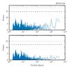 |
Fig. 4 Periodograms of the radial velocities of HD 21132, before (top) and after (bottom) correcting for a linear variation with |
HD 41248.
This star was the subject of a recent debate regarding the presence of a planetary system composed of two super-Earths. From an analysis of the first ~60 measurements of this dataset, Jenkins et al. (2013b) found evidence of two planets at orbital periods of 18.357 d and 25.648 d. Adding about 160 new radial-velocities, Santos et al. (2014) attributed one of the signals (25 d) to activity and could not recover convincing evidence for the second planet. More recently, Jenkins & Tuomi (2014) re-analysed the new data and again found the two-planet model to be the most probable. No new measurements were made for this star following the last two works, but we include it here for completeness.
The period at 25 d is found to be significant both in the periodogram and from the model selection analysis (with an odds ratio3 of ~6 × 10⁴). This would be very strong evidence in favour of (at least one) planetary companion. However, both the FWHM of the HARPS CCF and the show significant peaks at the same period (Fig. 5). In light of this evidence we must consider this signal to be caused by stellar activity (see also Suárez Mascareño et al. 2015).
The 18 d peak is not recovered clearly in the full dataset. In addition, a convincing detection of this planet presupposes a correction for the activity-induced signal. When attempting to perform this correction by removing sinusoids at 25 d and its harmonics, we do not find convincing evidence for the one-planet model. The orbital period of the reported planet, as detected by Jenkins & Tuomi (2014), is also very close to our estimate of the rotation period. It is clear that the currently available data do not allow a firm conclusion about the presence of a planetary system around HD 41248.
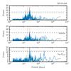 |
Fig. 5 Periodograms of the radial velocities, FWHM and |
HD 56274.
This star was followed closely for over 11 years with 228 observations in 161 nights. The RVs show a clear long-term modulation (Fig. 6), which is also evident from the periodogram (Fig. A.5). This modulation is correlated with the indicator (Fig. 7), which shows a clear long-term magnetic cycle. The periodogram of the values suggests a period of over ten years for this activity cycle.
From the relations of Noyes et al. (1984a) and Mamajek & Hillenbrand (2008), we estimate the rotation period of HD 56274 to be around 13 d (see Table 1). A peak at this period appears in the periodogram of the RV data, slightly above the 1% FAP line, but not in the observed values of the activity indicators. Interestingly, when removing a cubic polynomial from the values (as a correction for the magnetic cycle), a peak at 14.5 d appears in the periodogram of the residuals, although not at a significant level. This suggests that the rotation period of the star is indeed around 14 d, such that this signal is present in both RVs and the .
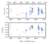 |
Fig. 6 Time series of the radial velocities (top) and |
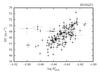 |
Fig. 7 Radial-velocity versus the |
To try to correct the RVs for the long-term activity-induced signal, we removed a linear correlation both with and with FWHM (which also correlates with the RVs). The periodograms of the corrected RVs are shown in Fig. 8. Correcting with removes most of the long-period peaks but leaves the peaks associated with one year aliases in the periodogram. The cause for these peaks is probably the same instrumental effect identified in the case of HD 88725 (see Sect. 4.3). No other significant signals can be found in the residual data. The correction with the FWHM reveals a significant peak at 14 d (close to the estimated rotation period) and two peaks at 62 d and 74 d. With this second correction, however, the long-term periodicities are not completely removed. We conclude that with the available data, and after correcting for the long-term magnetic cycle, it is not possible to confirm the presence of planets orbiting this star.
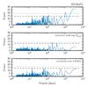 |
Fig. 8 Top panel: GLS periodogram of the observed radial-velocities of HD 56274. The middle and bottom panels show the periodograms after correcting the RVs from linear correlations with the |
HD 114076.
The rotation period for this star is estimated to be between 41 and 43 d, depending on the calibration (Table 1). The periodogram (Fig. 9 top panel, and Fig. A.6) shows a cluster of peaks around 40 d and also around 80 d. The strongest peak is at 41.3 d and very close to the 1% FAP.
To correct the RVs from what we believe is an activity-induced signal, a sine function was fitted and subtracted from the data. The best fit period was 41.27 d, and the periodogram of the residuals, shown in Fig. 9 (bottom panel), does not present additional significant signals.
To confirm that this signal is caused by the rotation of the star, we analysed the activity indicators. In particular, the shows a clear long-term trend, which might be caused by a magnetic cycle. We tried to remove the long-term variations by fitting both quadratic and cubic polynomials to the observations. The residuals of both fits show a clear periodic signal at 44.4 d, which helps to corroborate the activity-induced nature of the 41 d signal in the RVs.
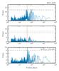 |
Fig. 9 Periodogram for HD 114076 before (top) and after (middle) fitting and removing a sine function to correct for activity-induced variations. The vertical dashed line indicates the best fit period of 41.27 d. The bottom plot shows the periodogram of the |
4.3. Sampling and instrumental effects
One additional obstacle in the detection of periodic RV variations due to planets is the presence of spurious signals and periodicities caused by the discrete time sampling of the observations or by instrumental effects. These can stem, amongst other effects, from Earth’s rotation and orbital motion. The following stars show evidence of contaminations of this kind.
HD 22879.
Although the periodogram of this star (Fig. A.7) does not show any significant peaks, the Bayesian analysis finds evidence of one Keplerian signal with a period of ~770 d and an eccentricity of 0.7. This corresponds to the second highest peak in the periodogram.
We find that this signal can, however, be caused by the time sampling of the observations. In the top and middle panels of Fig. 10, we show the periodogram together with the window function of the observations. The window function is calculated as the Fourier transform of the observation times (Roberts et al. 1987; Dawson & Fabrycky 2010), and it provides information on the power that is introduced in the periodogram due to the sampling.
The clean algorithm, introduced for frequency analysis by Roberts et al. (1987), is a well-known method of deconvolving the observed spectrum and the window function, thereby reducing the artefacts introduced by the sampling. Applying the clean algorithm to the RV measurements of HD 22879 results in the spectrum shown in the bottom panel of Fig. 10. The highest peak is at 14 d, which is close to the estimated stellar rotation period. It is not clear if this power is activity-induced, since the activity indicators do not show any clear signal at this period (or any long-term drifts).
We conclude that the Keplerian signal found at 770 d is best explained as originating in the time sampling. It is worth mentioning here that the Bayesian analysis is vulnerable to this kind of signal because it does not consider the information present in the window function at any stage.
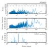 |
Fig. 10 Periodogram, window function, and CLEAN spectrum for the radial velocities of HD 22879. |
HD 79601.
The periodogram of the radial velocities of this star shows one significant peak at ~550 d (Fig. A.8). A Keplerian fit at this period results in a solution with P = 532.85 ± 9.63 d, a semi-amplitude of 1.92 ± 0.28 ms-1, and an eccentricity of 0.55 ± 0.18. A planet with these parameters would have a mass of 20.4 ± 4.16 M⊕. The phase-folded radial velocities for this solution (Fig. 11) show that the phase coverage is not ideal. The residuals from this fit do not show any significant periodogram peaks or evidence of any additional signals.
The lack of a good phase coverage of the orbital solution puts the planetary hypothesis in question. From Fig. A.8, it is clear that the measurements were obtained in several series, separated by large time gaps. Looking only at the observations after BJD = 2 454 500, the data show hints of a linear drift. When a linear drift is removed from this subset of the data (and also when a quadratic drift is removed from the full dataset), the peak at 550 d vanishes, and no other significant peaks remain in the periodogram of the residuals. At this point, our data do not allow us to reach any firm conclusions about the nature of the signal observed for HD 79601.
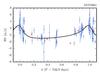 |
Fig. 11 Phase-folded radial-velocity measurements (blue) of HD 79601 with a period of 532.9 days. The red circles are the same radial velocities binned in phase with a bin size of 0.1, and the black line shows the best fit Keplerian function. |
HD 88725.
The radial velocities of this star show a significant periodicity at 368.3 d (Fig. A.9). Because this period is close to one year, we measured the correlation between the radial velocity and the barycentric Earth radial velocity (BERV). The posterior distribution for Spearman’s rank correlation coefficient (which was sampled using Markov chain Monte Carlo (MCMC); see Figueira et al. 2016) has a mean of –0.29, and a 95% credible interval (the highest posterior density interval) is [−0.46,−0.13 ]. This anti-correlation suggests that the signal detected in the RVs might be induced by the orbit of the Earth around the Sun.
Dumusque et al. (2015) recently described the cause for signals of this type to show up in HARPS radial velocities and suggested a method of correcting for this effect: the spectral lines that cross the so-called block stitchings in the HARPS CCD can be identified in the correlation mask used to derive the RVs. We created two different correlation masks, one with only the lines falling close to the block stitchings and one without those lines.
For the case of HD 88725, the periodograms of the RVs derived with the original mask and both custom masks are shown in Fig. 12. The spectral lines that cross the block stitching are the origin of the peak at one year (middle panel), and when those lines are removed from the correlation mask, the peak vanishes from the periodogram (bottom panel). After the RVs are corrected, the periodogram does not show significant peaks, and we do not find evidence of any Keplerian signals.
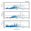 |
Fig. 12 Periodograms of the original radial velocities of HD 88725 (top panel), the radial velocities derived using a correlation mask that contains only the spectral lines crossing the CCD block stitchings (middle panel), and the radial velocities derived using a correlation mask without those lines (bottom panel). The vertical line shows the orbital period of the Earth. |
HD 111777.
In Fig. 13, the periodogram of the 79 measurements of this star is plotted together with the spectral window function (see also Fig. A.10). Although there are significant peaks in the periodogram, it becomes impossible to identify clear peaks produced by physical signals, because of the confusion introduced by the sampling. This does not mean that a long-period signal is not present, only that the highest peak in the periodogram can show up in a different location owing to the sampling.
Since the window function shows only excess power for long periods, and not distinct peaks, the CLEAN algorithm does not provide a good correction in this case. The large gap without observations is what causes these issues. After considering only the better-sampled subset of the data (after BJD = 2 456 000), we do not find any significant signals. Also, after removing a linear trend4 from the full dataset, the periodogram of the residuals does not show any significant peaks.
The periodograms of the activity indicators do not help in corroborating the presence of a planetary signal: the FWHM shows a non-significant periodicity close to 730 days, but the highest peak in the periodogram of the is at 16 days. For the case of HD 111777, we conclude that we are currently not able to assess the presence of a signal that might originate in a long-period planetary companion.
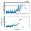 |
Fig. 13 Periodogram and window function for HD 111777. |
HD 224817.
The periodogram of the RVs of this star (Fig. A.11) does not show peaks above the 1% FAP line, but the model-selection analysis finds the model with one Keplerian to be the most probable. On the scale of Kass & Raftery (1995), an odds ratio of 1.25 (Table 4) is “not worth more than a bare mention”.
The highest peak in the periodogram is at ~245 d – the best-fit Keplerian also converges to this solution – but this period is probably caused by the deformation of the spectral lines that cross the block stitchings of the HARPS CCD, as for the case of HD 88725. We noticed this when fitting and removing a sinusoid with a period of one year from the RVs decreased the power of the 245 d peak.
To go on to check that the signal is indeed caused by the instrument, we created different correlation masks both with and without the lines falling close to the block stitchings (Dumusque et al. 2015). The periodograms for the original RVs and those from the two custom masks are shown in Fig. 14. When the spectral lines that cross the block stitchings are removed from the correlation mask, the 245 d peak vanishes from the periodogram (bottom panel). The periodogram of the corrected RVs does not show significant peaks, and we do not find evidence of any Keplerian signals.
Model selection results for the stars without significant periodogram peaks.
The second highest peak in the periodogram of the original radial velocities, around 10 d, is not far from the estimated rotation period of the star (Table 1). A clear (though not significant) peak at this period is present in the periodogram of the FWHM indicator. We conclude that the data available for HD 224817 does not suggest the presence of any planetary companions.
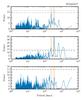 |
Fig. 14 Periodograms of the original radial velocities of HD 224817 (top panel), the RVs derived with a correlation mask that contains only the spectral lines crossing the CCD block stitchings (middle panel), and those derived using a correlation mask without those lines (bottom panel). The vertical lines show the period of the highest peak in the top periodogram and the orbital period of the Earth. |
4.4. Stars without identified signals
HD 31128.
This star was followed very closely with a total of 215 radial-velocity measurements on 169 different nights. These numbers already take an outlier observation at BJD = 2 455 304.48 into account, which was removed prior to the analysis. This observation has a very low CCF contrast value, making us suspect some instrumental or observational error at this date.
The RV data show high dispersion though the average uncertainty is also above 3 ms-1. These can be explained by the high effective temperature and very low metallicity of this star, which hinder the precise calculation of the radial-velocity with the CCF technique. Low-metallicity stars within this temperature range have shallower lines, making the determination of precise RVs more difficult, while the higher temperature introduces higher oscillation and granulation noise levels; Dumusque et al. 2011b.
Despite the large number of measurements, none of the periodogram peaks are significant (Fig. A.12). According to the model selection analysis, there is no evidence of any planetary companions orbiting this star. The constant model is preferred relative to the one-planet model according to the value of the evidence (with an odds ratio of 2.5) and the BIC (with ΔBIC of 5.4). However, the AICC selects instead the two-planet model, but in light of our general results (see Sect. 5), we tend to trust the Bayesian criteria.
HD 119173.
This star was observed on 98 different nights (totalling 128 measurements), which cover a total timespan of 8.1 years. No significant periodogram peaks were found (Fig. A.13), and in the model selection analysis, the constant model is preferred over the one-planet model (with odds ratio  and ΔBIC = 8.7). We conclude that there is no evidence for planetary signals in these data.
HD 119949.
The periodogram of the 81 measurements, shown in Fig. A.14, does not present any significant peaks. The Bayesian search for Keplerian signals reaches the same conclusions (odds ratio  ). The AICC again selects a more complex one-planet model with a non-significant ΔAICC. We report no clear evidence for planetary companions.
HD 126793.
A total of 96 measurements on 79 different nights were obtained. The periodogram (Fig. A.15) does not show any significant peaks, and in this case as well, the model comparison does not find evidence for Keplerian signals in the data. For these data, all model selection criteria select the constant model as the most probable with , ΔAICC= 1.1, ΔBIC = 11.5.
5. Comparison of model selection criteria
For the maximum-likelihood solutions, the AICC and BIC can be calculated using the number of free parameters in a given model. They are sometimes used as model-selection criteria and are much easier to calculate than the value of the evidence. In Table 4 we show the AICC and BIC values for each star and model, using the maximum-likelihood obtained from all MultiNest samples. We highlight in bold the best model according to each criteria.
As general trends in our results we can note that the AICC tends to choose a model with a higher number of Keplerian signals. The BIC is found to be more conservative and tends to agree with the model with the highest evidence. These results suggest that the BIC can be used as a viable approximation to the evidence, given that the (global) maximum of the likelihood function can be found.
6. Detection limits
Many of the stars we analysed in Sect. 4 do not contain significant periodic signals or show signals stemming from activity and sampling contaminations. In this section, we derive upper limits to the planetary signals that can be present and yet still undetectable in these data. For any given star, we determine which planet, as a function of its mass and orbital period, can already be ruled out with our observations.
The detection limits are calculated with a standard procedure: injecting trial circular orbits into the observed data (Cumming et al. 1999; Endl et al. 2001; Zechmeister et al. 2009; Dumusque et al. 2011c; Mayor et al. 2011; Mortier et al. 2012). We explore all periods in the range from 1 d to 500 d and semi-amplitudes from 0 to 10 ms-1 (using a binary search). For ten linearly spaced phases, we compare the periodogram power of the injected period with the FAP level of that period in the original dataset. If, for all phases, the former is higher we consider the planet to be detected. We convert the semi-amplitude to planetary mass using the stellar masses listed in Table 1.
It is important to note that this method assumes that the original dataset (in which mock planets are injected) only contains uncorrelated noise. For the stars analysed in Sect. 4.4, this assumption is valid. For the stars analysed in Sect. 4.1, we substracted the putative orbital solution from the data before calculating the detection limits. Since correcting for activity-induced signals and artefacts originating in the sampling is much more prone to error, for the stars discussed in Sects. 4.2 and 4.3, we assume that the observed radial-velocities contain only noise. Therefore, for this last group of stars, the detection limits estimates can be taken as conservative.
The 99% detection limits for all 15 stars are shown in Fig. 15 where we highlight the regions corresponding to planets with P< 50 d, and masses in the ranges M = 10−30 M⊕ and M = 30−100 M⊕. These can be compared to the same regions considered in (Mayor et al. 2011) for the calculation of the planet ocurrence rate.
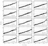 |
Fig. 15 Detection limits for the 15 stars studied in this work. The plots show planetary mass against orbital period. The thick black line shows the 99% detection limits, estimated by injecting trial circular orbits. The dashed blue lines represent circular planetary signals with RV semi-amplitudes of 1, 3, and 5 ms-1 (from bottom to top in each panel). The regions delimited by the red dotted lines correspond to periods lower than 50 d, and masses in the ranges M = 10−30 M⊕ and M = 30−100 M⊕. |
Almost uniformly in this sample, we are sensitive to planets that are more massive than 10 M⊕ up to orbital periods of 50 days. For shorter period planets, with P ~ 10 days and less, the current data would already allow for detecting planets with just a few Earth masses.
7. Discussion and conclusions
From over 100 targets in our metal-poor large programme, we selected those that were observed on more than 75 nights. A homogeneous analysis of the radial-velocity observations was carried out by comparing models with a varying number of Keplerian signals. We used the nested sampling algorithm to estimate the evidence of a given model and compared the results with the posterior distribution of the number of Keplerians n. We also calculated the AICC and BIC and analysed the periodograms of the radial velocities and activity indicators.
In some cases,we find a disagreement between the evidence results and the presence of significant periodogram peaks. The Bayesian analysis was able to identify a few Keplerian signals that are not significant in the periodograms. Nevertheless, the values of the odds ratios indicate that these detections are not very significant. The results obtained with MultiNest almost always5 agree with the posterior distribution p(n | d), which is reassuring but not surprising given that the same priors and likelihood were used in both algorithms.
Signals induced by stellar activity were detected for HD 21132, HD 56274, and HD 114076, besides the known case of HD 41248. After attempting to correct for these signals, we were not able to recover any additional signs of planetary companions.
For HD 79601, HD 22879, and HD 111777, the time sampling of the observations induces spurious signals in the radial velocities, hindering the detection of planetary signals. We also identified a clear one-year periodicity and its harmonics, caused by instrumental effects, on the radial velocities of HD 88725 and HD 224817. These instrument-induced RV variations are not expected to be present in all stars since each star may have different values of the BERV and different spectral lines crossing the CCD block stitchings (see Dumusque et al. 2015).
HD 87838 shows an interesting signal around 68 d, which can be fitted with a slightly eccentric Keplerian. The model selection does not provide strong evidence for the presence of this planet, but we hope to obtain more data to assert its nature. It is important to note that the value of the evidence (and our estimate) is sensitive to the priors on the parameters of a given model. This is not necessarily a limitation, meaning only that care should be taken when choosing the priors and that they should be stated clearly in any analysis.
As an example of these points, we analysed the data of HD 87838 again with n = 1, considering the prior for the orbital period to be uniform between 65 d and 75 d6. The resulting value for the evidence was found to be −209.5, in contrast to the value determined previously, of −213.9 (Table 4). This corresponds to an odds ratio of ~156 against the constant model, which would imply very strong evidence for a Keplerian signal and a confident planet detection.
We performed a sensitivity analysis of our results, namely by considering different priors for the orbital periods and semi-amplitudes. Even if, in some cases, a different model was preferred (that is, yielded a stronger proof), the absolute value of the Bayes factors did not change considerably. This means that our level of confidence in the presence or not of a planetary signal does not strictly depend on the parameter priors.
Even though our working sample is small, it already allows for an analysis of the frequency of planets around these stars. We do not attempt to provide constraints on the planet frequency as a function of stellar metallicity, since our sample does not span the metallicity space completely (Fig. 1).
The probability of obtaining k detections in a sample of size N is given by the binomial distribution, assuming a planet frequency fp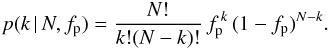 (5)This equation can be thought of as a function of fp for given values of k and N, therefore representing a (un-normalised) posterior distribution for fp. The number of planets detected in a given sample places a constraint on the probable values of the planet frequency, which can be expressed by the mode and the range that covers 68% of the distribution, for example.
Considering the detection of the planet orbiting HD 175607 in a sample of 15 stars, this procedure gives a constraint of  . Taking also the unconfirmed planet around HD 87838 into account, one obtains
  . This last result agrees with that of Mayor et al. (2011), who found 12.27 ± 2.45% for the combined occurrence rate of planets with orbital periods shorter than 50 days and masses in the range M = 10−100 M⊕. We nevertheless stress that our constraints on the planet occurrence rate are preliminary, since they are based on a small sample and subject to selection biases.
Recent studies have identified correlations between the properties of the planetary system and the metallicity of the star. Lower metallicity stars have been found to host longer period planets (Beaugé & Nesvorný 2013; Adibekyan et al. 2013) or lower eccentricity orbits (Dawson & Murray-Clay 2013). These results, together with the detection limits calculated in Sect. 6, might explain why few planets have been detected so far in our sample. The search for low-mass planets around metal-poor stars requires not only high-precision radial velocities but also a very long baseline of observations.
Our results show that the detection of small planets in these data is hindered by time sampling problems and activity-induced signals. Careful planning of the observational strategy and detailed analyses of the aliasing structures are needed to mitigate some of these problems, and we must seek ways to make use of all the information contained in the RVs and in all the activity indicators, in an optimal and physically meaningful way.
The analysis of the full sample of 109 metal-poor stars is ongoing, and we expect to provide constraints on the frequency of planets orbiting these stars when the observations of the Large Program are finished.
The prior mass element is dX = p(Θ | Mn)dΘ such that E = ∫L dX, with L the likelihood function.
In our full sample, the highest radial-velocity rms is 4.1 ms-1.
The odds ratio cannot be compared to the one found by Jenkins & Tuomi (2014) because we did not use the same model for the RVs.
For consistency, we checked that the evidence of the constant model is higher than that of a model with an added linear drift parameter.
The exceptions are the 2-planet models for HD 87838 and HD 224817. This can be due to poorer sampling by one of the algorithms or incomplete convergence.
The example is contrived but might shed light on why one should not adjust the priors after having looked at the data (or the periodogram, for that matter).
Acknowledgments
We would like to thank the referee, Dr. Silvano Desidera, for a careful reading and insightful comments on the paper that helped to improve its quality. This work was supported by Fundação para a Ciência e a Tecnologia (FCT) through the research grant UID/FIS/04434/2013. We also acknowledge the support from FCT in the form of grant reference PTDC/FIS-AST/1526/2014. J.P.F. acknowledges the support from FCT through the grant reference SFRH/BD/93848/2013 and thanks Brendon Brewer for his assistance with the diffusive nested sampling code. P.F. and N.C.S. acknowledge support by FCT through Investigador FCT contracts of reference IF/01037/2013 and IF/00169/2012, respectively, and POPH/FSE (EC) by FEDER funding through the program “Programa Operacional de Factores de Competitividade – COMPETE”. P.F. further acknowledges support from FCT in the form of an exploratory project of reference IF/01037/2013CP1191/CT0001. A.M. received funding from the European Union Seventh Framework Program (FP7/2007-2013) under grant agreement number 313014 (ETAEARTH). A.S. is supported by the European Union under a Marie Curie Intra-European Fellowship for Career Development with reference FP7-PEOPLE-2013-IEF, number 627202.
References
- Adibekyan, V. Z., Delgado Mena, E., Sousa, S. G., et al. 2012, A&A, 547, A36 [NASA ADS] [CrossRef] [EDP Sciences] [Google Scholar]
- Adibekyan, V. Z., Figueira, P., Santos, N. C., et al. 2013, A&A, 560, A51 [NASA ADS] [CrossRef] [EDP Sciences] [Google Scholar]
- Adibekyan, V., Santos, N. C., Figueira, P., et al. 2015, A&A, 581, L2 [NASA ADS] [CrossRef] [EDP Sciences] [Google Scholar]
- Baliunas, S. L., Donahue, R. A., Soon, W. H., et al. 1995, ApJ, 438, 269 [NASA ADS] [CrossRef] [Google Scholar]
- Baranne, A., Queloz, D., Mayor, M., et al. 1996, A&AS, 119, 373 [NASA ADS] [CrossRef] [EDP Sciences] [Google Scholar]
- Beaugé, C., & Nesvorný, D. 2013, ApJ, 763, 12 [NASA ADS] [CrossRef] [Google Scholar]
- Boisse, I., Bouchy, F., Hébrard, G., et al. 2011, A&A, 528, A4 [NASA ADS] [CrossRef] [EDP Sciences] [Google Scholar]
- Bonfils, X., Mayor, M., Delfosse, X., et al. 2007, A&A, 474, 293 [NASA ADS] [CrossRef] [EDP Sciences] [Google Scholar]
- Brewer, B. J., & Donovan, C. P. 2015, MNRAS, 448, 3206 [NASA ADS] [CrossRef] [Google Scholar]
- Brewer, B. J., Pártay, L. B., & Csányi, G. 2011, Stat. Comput., 21, 649 [Google Scholar]
- Buchhave, L. A., & Latham, D. W. 2015, ApJ, 808, 187 [NASA ADS] [CrossRef] [Google Scholar]
- Buchhave, L. A., Latham, D. W., Johansen, A., et al. 2012, Nature, 486, 375 [NASA ADS] [Google Scholar]
- Burnham, K. P., & Anderson, D. R. 2010, Model Selection and Multimodel Inference, 2nd edn. (Springer) [Google Scholar]
- Cumming, A., Marcy, G. W., & Butler, R. P. 1999, ApJ, 526, 890 [NASA ADS] [CrossRef] [Google Scholar]
- Dawson, R. I., & Fabrycky, D. C. 2010, ApJ, 722, 937 [NASA ADS] [CrossRef] [Google Scholar]
- Dawson, R. I., & Murray-Clay, R. A. 2013, ApJ, 767, L24 [NASA ADS] [CrossRef] [Google Scholar]
- Dawson, R. I., Chiang, E., & Lee, E. J. 2015, MNRAS, 453, 1471 [NASA ADS] [CrossRef] [Google Scholar]
- Dumusque, X., Lovis, C., Ségransan, D., et al. 2011a, A&A, 535, A55 [NASA ADS] [CrossRef] [EDP Sciences] [Google Scholar]
- Dumusque, X., Santos, N. C., Udry, S., Lovis, C., & Bonfils, X. 2011b, A&A, 527, A82 [NASA ADS] [CrossRef] [EDP Sciences] [Google Scholar]
- Dumusque, X., Udry, S., Lovis, C., Santos, N. C., & Monteiro, M. J. P. F. G. 2011c, A&A, 525, A140 [NASA ADS] [CrossRef] [EDP Sciences] [Google Scholar]
- Dumusque, X., Pepe, F., Lovis, C., et al. 2012, Nature, 491, 207 [NASA ADS] [CrossRef] [PubMed] [Google Scholar]
- Dumusque, X., Pepe, F., Lovis, C., & Latham, D. W. 2015, ApJ, 808, 171 [NASA ADS] [CrossRef] [Google Scholar]
- Endl, M., Kürster, M., Els, S., Hatzes, A. P., & Cochran, W. D. 2001, A&A, 374, 675 [NASA ADS] [CrossRef] [EDP Sciences] [Google Scholar]
- Feroz, F., & Hobson, M. P. 2014, MNRAS, 437, 3540 [NASA ADS] [CrossRef] [Google Scholar]
- Feroz, F., Hobson, M. P., & Bridges, M. 2009, MNRAS, 398, 1601 [NASA ADS] [CrossRef] [Google Scholar]
- Feroz, F., Balan, S. T., & Hobson, M. P. 2011a, MNRAS, 416, L104 [NASA ADS] [CrossRef] [Google Scholar]
- Feroz, F., Balan, S. T., & Hobson, M. P. 2011b, MNRAS, 415, 3462 [NASA ADS] [CrossRef] [Google Scholar]
- Feroz, F., Hobson, M. P., Cameron, E., & Pettitt, A. N. 2013, ArXiv e-prints [arXiv:1306.2144] [Google Scholar]
- Figueira, P., Faria, J. P., Adibekyan, V. Z., Oshagh, M., & Santos, N. C. 2016, ArXiv e-prints [arXiv:1601.05107] [Google Scholar]
- Fischer, D. A., & Valenti, J. 2005, ApJ, 622, 1102 [NASA ADS] [CrossRef] [Google Scholar]
- Gonzalez, G. 1997, MNRAS, 285, 403 [NASA ADS] [CrossRef] [Google Scholar]
- Gregory, P. C. 2007, MNRAS, 374, 1321 [NASA ADS] [CrossRef] [Google Scholar]
- Gregory, P. C. 2010, Bayesian logical data analysis for the physical sciences (Cambridge University Press) [Google Scholar]
- Grunblatt, S. K., Howard, A. W., & Haywood, R. D. 2015, ApJ, 808, 127 [NASA ADS] [CrossRef] [Google Scholar]
- Guillot, T., Santos, N. C., Pont, F., et al. 2006, A&A, 453, L21 [NASA ADS] [CrossRef] [EDP Sciences] [Google Scholar]
- Hatzes, A. P. 2014, A&A, 568, A84 [NASA ADS] [CrossRef] [EDP Sciences] [Google Scholar]
- Ida, S., & Lin, D. N. C. 2004, ApJ, 616, 567 [NASA ADS] [CrossRef] [MathSciNet] [Google Scholar]
- Jenkins, J. S., & Tuomi, M. 2014, ApJ, 794, 110 [NASA ADS] [CrossRef] [Google Scholar]
- Jenkins, J. S., Jones, H. R. A., Tuomi, M., et al. 2013a, ApJ, 766, 67 [NASA ADS] [CrossRef] [Google Scholar]
- Jenkins, J. S., Tuomi, M., Brasser, R., Ivanyuk, O., & Murgas, F. 2013b, ApJ, 771, 41 [NASA ADS] [CrossRef] [Google Scholar]
- Kass, R. E., & Raftery, A. E. 1995, J. Am. Stat. Assoc., 90, 773 [Google Scholar]
- Kipping, D. M. 2013, MNRAS, 434, L51 [NASA ADS] [CrossRef] [Google Scholar]
- Lovis, C., Dumusque, X., Santos, N. C., et al. 2011, ArXiv e-prints [arXiv:1107.5325] [Google Scholar]
- Mamajek, E. E., & Hillenbrand, L. A. 2008, ApJ, 687, 1264 [NASA ADS] [CrossRef] [Google Scholar]
- Mayor, M., Marmier, M., Lovis, C., et al. 2011, A&A, submitted [arXiv:1109.2497] [Google Scholar]
- Melo, C., Santos, N. C., Gieren, W., et al. 2007, A&A, 467, 721 [NASA ADS] [CrossRef] [EDP Sciences] [Google Scholar]
- Mordasini, C., Alibert, Y., Benz, W., & Naef, D. 2009, A&A, 501, 1161 [NASA ADS] [CrossRef] [EDP Sciences] [Google Scholar]
- Mordasini, C., Mollière, P., Dittkrist, K.-M., Jin, S., & Alibert, Y. 2015, Int. J. Astrobiol., 14, 201 [CrossRef] [Google Scholar]
- Mortier, A., Santos, N. C., Sozzetti, A., et al. 2012, A&A, 543, A45 [NASA ADS] [CrossRef] [EDP Sciences] [Google Scholar]
- Mortier, A., Santos, N. C., Sousa, S., et al. 2013, A&A, 551, A112 [NASA ADS] [CrossRef] [EDP Sciences] [Google Scholar]
- Mortier, A., Faria, J. P., Santos, N. C., et al. 2016, A&A, 585, A135 [NASA ADS] [CrossRef] [EDP Sciences] [Google Scholar]
- Mukherjee, P., Parkinson, D., & Liddle, A. R. 2006, ApJ, 638, L51 [Google Scholar]
- Murdoch, K. A., Hearnshaw, J. B., & Clark, M. 1993, ApJ, 413, 349 [NASA ADS] [CrossRef] [Google Scholar]
- Naef, D., Mayor, M., Benz, W., et al. 2007, A&A, 470, 721 [NASA ADS] [CrossRef] [EDP Sciences] [Google Scholar]
- Neves, V., Bonfils, X., Santos, N. C., et al. 2013, A&A, 551, A36 [NASA ADS] [CrossRef] [EDP Sciences] [Google Scholar]
- Noyes, R. W., Hartmann, L. W., Baliunas, S. L., Duncan, D. K., & Vaughan, A. H. 1984a, ApJ, 279, 763 [NASA ADS] [CrossRef] [Google Scholar]
- Noyes, R. W., Weiss, N. O., & Vaughan, A. H. 1984b, ApJ, 287, 769 [NASA ADS] [CrossRef] [Google Scholar]
- Pepe, F., Mayor, M., Galland, F., et al. 2002, A&A, 388, 632 [NASA ADS] [CrossRef] [EDP Sciences] [Google Scholar]
- Perryman, M. A. C. 2014, The Exoplanet Handbook, 1st edn. (Cambridge University Press) [Google Scholar]
- Queloz, D., Henry, G. W., Sivan, J. P., et al. 2001, A&A, 379, 279 [NASA ADS] [CrossRef] [EDP Sciences] [Google Scholar]
- Roberts, D. H., Lehar, J., & Dreher, J. W. 1987, AJ, 93, 968 [NASA ADS] [CrossRef] [Google Scholar]
- Robertson, P., & Mahadevan, S. 2014, ApJ, 793, L24 [NASA ADS] [CrossRef] [Google Scholar]
- Santos, N. C., Mayor, M., Naef, D., et al. 2000, A&A, 361, 265 [NASA ADS] [Google Scholar]
- Santos, N. C., Israelian, G., & Mayor, M. 2004, A&A, 415, 1153 [NASA ADS] [CrossRef] [EDP Sciences] [Google Scholar]
- Santos, N. C., Mayor, M., Bouchy, F., et al. 2007, A&A, 474, 647 [NASA ADS] [CrossRef] [EDP Sciences] [Google Scholar]
- Santos, N. C., Mayor, M., Bonfils, X., et al. 2011, A&A, 526, A112 [NASA ADS] [CrossRef] [EDP Sciences] [Google Scholar]
- Santos, N. C., Mortier, A., Faria, J. P., et al. 2014, A&A, 566, A35 [NASA ADS] [CrossRef] [EDP Sciences] [Google Scholar]
- Santos, N. C., Adibekyan, V., Mordasini, C., et al. 2015, A&A, 580, L13 [NASA ADS] [CrossRef] [EDP Sciences] [Google Scholar]
- Schneider, J., Dedieu, C., Le Sidaner, P., Savalle, R., & Zolotukhin, I. 2011, A&A, 532, A79 [NASA ADS] [CrossRef] [EDP Sciences] [Google Scholar]
- Sivia, D. S., & Skilling, J. 2006, Data Analysis: A Bayesian Tutorial (Oxford: Oxford University Press) [Google Scholar]
- Skilling, J. 2004, in Bayesian Inference and Maximum Entropy Methods in Science and Engineering, AIP Conf. Proc., 735, 395 [Google Scholar]
- Sousa, S. G., Santos, N. C., Mayor, M., et al. 2008, A&A, 487, 373 [NASA ADS] [CrossRef] [EDP Sciences] [MathSciNet] [Google Scholar]
- Sousa, S. G., Santos, N. C., Israelian, G., et al. 2011a, A&A, 526, A99 [NASA ADS] [CrossRef] [EDP Sciences] [Google Scholar]
- Sousa, S. G., Santos, N. C., Israelian, G., Mayor, M., & Udry, S. 2011b, A&A, 533, A141 [NASA ADS] [CrossRef] [EDP Sciences] [Google Scholar]
- Sozzetti, A., Torres, G., Latham, D. W., et al. 2009, ApJ, 697, 544 [NASA ADS] [CrossRef] [Google Scholar]
- Suárez Mascareño, A., Rebolo, R., González Hernández, J. I., & Esposito, M. 2015, MNRAS, 452, 2745 [NASA ADS] [CrossRef] [Google Scholar]
- Tinney, C. G., Butler, R. P., Marcy, G. W., et al. 2002, ApJ, 571, 528 [NASA ADS] [CrossRef] [Google Scholar]
- Udry, S., & Santos, N. C. 2007, ARA&A, 45, 397 [NASA ADS] [CrossRef] [Google Scholar]
- Udry, S., Mayor, M., Benz, W., et al. 2006, A&A, 447, 361 [NASA ADS] [CrossRef] [EDP Sciences] [Google Scholar]
- Wang, J., & Fischer, D. A. 2014, AJ, 149, 14 [Google Scholar]
- Zechmeister, M., & Kürster, M. 2009, A&A, 496, 577 [NASA ADS] [CrossRef] [EDP Sciences] [Google Scholar]
- Zechmeister, M., Kürster, M., & Endl, M. 2009, A&A, 505, 859 [NASA ADS] [CrossRef] [EDP Sciences] [Google Scholar]
Appendix A: RV time series and periodograms
This appendix contains figures with the radial-velocity time series and respective GLS periodogram for each star.
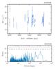 |
Fig. A.1 Radial-velocity time series and periodogram for HD 87838. |
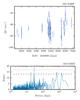 |
Fig. A.2 Radial-velocity time series and periodogram for HD 175607. |
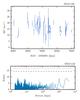 |
Fig. A.3 Radial-velocity time series and periodogram for HD 21132. |
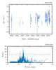 |
Fig. A.4 Radial-velocity time series and periodogram for HD 41248. |
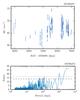 |
Fig. A.5 Radial-velocity time series and periodogram for HD 56274. |
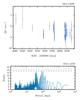 |
Fig. A.6 Radial-velocity time series and periodogram for HD 114076. |
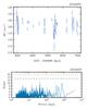 |
Fig. A.7 Radial-velocity time series and periodogram for HD 22879. |
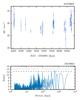 |
Fig. A.8 Radial-velocity time series and periodogram for HD 79601. |
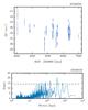 |
Fig. A.9 Radial-velocity time series and periodogram for HD 88725. |
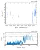 |
Fig. A.10 Radial-velocity time series and periodogram for HD 111777. |
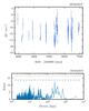 |
Fig. A.11 Radial-velocity time series and periodogram for HD 224817. |
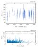 |
Fig. A.12 Radial-velocity time series and periodogram for HD 31128. |
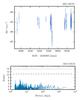 |
Fig. A.13 Radial-velocity time series and periodogram for HD 119173. |
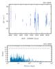 |
Fig. A.14 Radial-velocity time series and periodogram for HD 119949. |
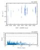 |
Fig. A.15 Radial-velocity time series and periodogram for HD 126793. |
All Tables
Number of individual night observations, average RV errorbar, weighted standard deviation of the RV measurements, and timespan for each of the targets.
All Figures
|
Fig. 1 Metallicity, effective temperature, and surface gravity distributions for the full metal-poor sample (blue histograms) and the 15 stars observed on more than 75 different nights (green filled histograms). |
| In the text | |
|
Fig. 2 Phase-folded RV curve for HD 87838 with a period of 68.42 d. The blue points indicate the measured radial-velocities, and red circles show the same radial velocities binned in phase with a bin size of 0.1. |
| In the text | |
|
Fig. 3 Periodograms of the radial velocities (top) the |
| In the text | |
|
Fig. 4 Periodograms of the radial velocities of HD 21132, before (top) and after (bottom) correcting for a linear variation with |
| In the text | |
|
Fig. 5 Periodograms of the radial velocities, FWHM and |
| In the text | |
|
Fig. 6 Time series of the radial velocities (top) and |
| In the text | |
|
Fig. 7 Radial-velocity versus the |
| In the text | |
|
Fig. 8 Top panel: GLS periodogram of the observed radial-velocities of HD 56274. The middle and bottom panels show the periodograms after correcting the RVs from linear correlations with the |
| In the text | |
|
Fig. 9 Periodogram for HD 114076 before (top) and after (middle) fitting and removing a sine function to correct for activity-induced variations. The vertical dashed line indicates the best fit period of 41.27 d. The bottom plot shows the periodogram of the |
| In the text | |
|
Fig. 10 Periodogram, window function, and CLEAN spectrum for the radial velocities of HD 22879. |
| In the text | |
|
Fig. 11 Phase-folded radial-velocity measurements (blue) of HD 79601 with a period of 532.9 days. The red circles are the same radial velocities binned in phase with a bin size of 0.1, and the black line shows the best fit Keplerian function. |
| In the text | |
|
Fig. 12 Periodograms of the original radial velocities of HD 88725 (top panel), the radial velocities derived using a correlation mask that contains only the spectral lines crossing the CCD block stitchings (middle panel), and the radial velocities derived using a correlation mask without those lines (bottom panel). The vertical line shows the orbital period of the Earth. |
| In the text | |
|
Fig. 13 Periodogram and window function for HD 111777. |
| In the text | |
|
Fig. 14 Periodograms of the original radial velocities of HD 224817 (top panel), the RVs derived with a correlation mask that contains only the spectral lines crossing the CCD block stitchings (middle panel), and those derived using a correlation mask without those lines (bottom panel). The vertical lines show the period of the highest peak in the top periodogram and the orbital period of the Earth. |
| In the text | |
|
Fig. 15 Detection limits for the 15 stars studied in this work. The plots show planetary mass against orbital period. The thick black line shows the 99% detection limits, estimated by injecting trial circular orbits. The dashed blue lines represent circular planetary signals with RV semi-amplitudes of 1, 3, and 5 ms-1 (from bottom to top in each panel). The regions delimited by the red dotted lines correspond to periods lower than 50 d, and masses in the ranges M = 10−30 M⊕ and M = 30−100 M⊕. |
| In the text | |
|
Fig. A.1 Radial-velocity time series and periodogram for HD 87838. |
| In the text | |
|
Fig. A.2 Radial-velocity time series and periodogram for HD 175607. |
| In the text | |
|
Fig. A.3 Radial-velocity time series and periodogram for HD 21132. |
| In the text | |
|
Fig. A.4 Radial-velocity time series and periodogram for HD 41248. |
| In the text | |
|
Fig. A.5 Radial-velocity time series and periodogram for HD 56274. |
| In the text | |
|
Fig. A.6 Radial-velocity time series and periodogram for HD 114076. |
| In the text | |
|
Fig. A.7 Radial-velocity time series and periodogram for HD 22879. |
| In the text | |
|
Fig. A.8 Radial-velocity time series and periodogram for HD 79601. |
| In the text | |
|
Fig. A.9 Radial-velocity time series and periodogram for HD 88725. |
| In the text | |
|
Fig. A.10 Radial-velocity time series and periodogram for HD 111777. |
| In the text | |
|
Fig. A.11 Radial-velocity time series and periodogram for HD 224817. |
| In the text | |
|
Fig. A.12 Radial-velocity time series and periodogram for HD 31128. |
| In the text | |
|
Fig. A.13 Radial-velocity time series and periodogram for HD 119173. |
| In the text | |
|
Fig. A.14 Radial-velocity time series and periodogram for HD 119949. |
| In the text | |
|
Fig. A.15 Radial-velocity time series and periodogram for HD 126793. |
| In the text | |
Current usage metrics show cumulative count of Article Views (full-text article views including HTML views, PDF and ePub downloads, according to the available data) and Abstracts Views on Vision4Press platform.
Data correspond to usage on the plateform after 2015. The current usage metrics is available 48-96 hours after online publication and is updated daily on week days.
Initial download of the metrics may take a while.