| Issue |
A&A
Volume 589, May 2016
|
|
|---|---|---|
| Article Number | A14 | |
| Number of page(s) | 25 | |
| Section | Stellar structure and evolution | |
| DOI | https://doi.org/10.1051/0004-6361/201424740 | |
| Published online | 05 April 2016 | |
Revealing the broad iron Kα line in Cygnus X-1 through simultaneous XMM-Newton, RXTE, and INTEGRAL observations
1 Dr. Karl Remeis-Sternwarte and Erlangen Centre for Astroparticle Physics, Friedrich-Alexander-Universität Erlangen-Nürnberg, Sternwartstraße 7, 96049 Bamberg, Germany
e-mail: This email address is being protected from spambots. You need JavaScript enabled to view it.
2 AIT Austrian Institute of Technology GmbH, Donau-City-Straße 1, 1220 Vienna, Austria
3 Kavli Institute for Astrophysics, Massachusetts Institute of Technology, Cambridge, MA 02139, USA
4 Laboratoire AIM, CEA/IRFU-Université Paris Diderot-CNRS/INSU, CEA DSM/IRFU/SAp, Centre de Saclay, 91191 Gif-sur-Yvette, France
5 Space Sciences Laboratory, University of California, 7 Gauss Way, Berkeley, CA 94720, USA
6 CRESST and NASA Goddard Space Flight Center, Astrophysics Science Division, Code 661, Greenbelt, MD 20771, USA
7 Center for Space Science and Technology, University of Maryland Baltimore County, 1000 Hilltop Circle, Baltimore, MD 21250, USA
8 Institut für Astronomie und Astrophysik, Eberhard Karls Universität Tübingen, Sand 1, 72074 Tübingen, Germany
9 Max Planck Computing and Data Facility, Gießenbachstraße 2, 85748 Garching, Germany
10 Department of Chemistry, Physics, and Astronomy, Georgia College, CBX 082, Milledgeville, GA 31061, USA
11 Institute of Astronomy, Madingley Road, Cambridge CB3 0HA, UK
12 Department of Astronomy and Maryland Astronomy Center for Theory and Computation, University of Maryland, College Park, MD 20742, USA
13 European Space Agency, European Space Operations Centre, Robert-Bosch-Straße 5, 64293 Darmstadt, Germany
Received: 4 August 2014
Accepted: 20 February 2016
Abstract
We report on the analysis of the broad Fe Kα line feature of Cyg X-1 in the spectra of four simultaneous hard intermediate state observations made with the X-ray Multiple Mirror mission (XMM-Newton), the Rossi X-ray Timing Explorer (RXTE), and the International Gamma-Ray Astrophysics Laboratory (INTEGRAL). The high quality of the XMM-Newton data taken in the Modified Timing Mode of the EPIC-pn camera provides a great opportunity to investigate the broadened Fe Kα reflection line at 6.4 keV with a very high signal to noise ratio. The 4–500 keV energy range is used to constrain the underlying continuum and the reflection at higher energies. We first investigate the data by applying a phenomenological model that consists of the sum of an exponentially cutoff power law and relativistically smeared reflection. Additionally, we apply a more physical approach and model the irradiation of the accretion disk directly from the lamp post geometry. All four observations show consistent values for the black hole parameters with a spin of a ~ 0.9, in agreement with recent measurements from reflection and disk continuum fitting. The inclination is found to be i ~ 30°, consistent with the orbital inclination and different from inclination measurements made during the soft state, which show a higher inclination. We speculate that the difference between the inclination measurements is due to changes in the inner region of the accretion disk.
Key words: X-rays: binaries / black hole physics / gravitation
Deceased 2 September 2015.
© ESO, 2016
1. Introduction
The high mass X-ray binary system Cyg X-1 (Bowyer et al. 1965; Murdin & Webster 1971) consists of a 14.8 ± 1.0 M⊙ black hole and the 19.2 ± 1.9 M⊙ OB giant star HDE 226868 (Orosz et al. 2011, but see also Ziółkowski 2014). The system is at a distance of d ~ 1.86 kpc (Reid et al. 2011; Xiang et al. 2011). The orbital period of the system is 5.6 d (Webster & Murdin 1972; Bolton 1972) at an inclination of  (Orosz et al. 2011). Recently, several groups reported a very high spin of a ~ 0.9 for Cyg X-1 (Duro et al. 2011; Gou et al. 2011; Fabian et al. 2012). The donor star HDE 226868 is close to filling its Roche lobe (Gies & Bolton 1986), creating a focused wind towards the black hole (Friend & Castor 1982), where the wind material forms an accretion disk. The observed X-ray flux from the disk is orbital-phase dependent, since the wind material can absorb a significant amount of the flux, resulting in spectral absorption and, in the most extreme cases, dips in the lightcurves of the observed object (see, e.g., Grinberg et al. 2015; Miškovičová et al. 2016; Hanke et al. 2009; Díaz Trigo et al. 2006; Bałucińska-Church et al. 2000).
Historically, Cyg X-1 has spent most of its time in the low luminosity “hard state” (Wilms et al. 2006a; Grinberg et al. 2013), in which the X-ray spectrum above ~2 keV is well described by an exponentially cutoff power-law with a photon index of Γ ~ 1.7 and an exponential folding energy of Efold ~ 150 keV (Sunyaev & Trümper 1979; Wilms et al. 2006a; Nowak et al. 2011), and a very weak disk component. The power-law emission originates in a corona or a jet (e.g., Nowak et al. 2011). Radio emission is detected during the hard state and is attributed to synchrotron emission from electrons in a relativistic outflow (Stirling et al. 2001; Malzac et al. 2009). Synchrotron radiation is also the likely cause for the hard tail seen at >400 keV (McConnell et al. 1994, 2000; Cadolle Bel et al. 2006), which is strongly polarized (Laurent et al. 2011; Jourdain et al. 2012). In the “soft state” the spectrum can be described by thermal emission from a 0.5–0.6 keV standard accretion disk (see, e.g., Tomsick et al. 2014), a steep power-law photon index, and no high energy cutoff. Occasional transitions and failed transitions from one to the other state define a “hard (or soft) intermediate state”, that is characterized by distinct spectral and variability properties (Pottschmidt et al. 2003; Grinberg et al. 2014).
The behavior of Cyg X-1 can be explained by the underlying geometry of an accreting black hole. In the standard view, the black hole is surrounded by an accretion disk that is illuminated by photons from a corona or the base of a jet, which is located close to the black hole. At the inner edge of the accretion disk, the temperature is typically a few 100 eV. A fraction of the disk’s thermal emission is intercepted by the thermal (or hybrid) hot gas in the vicinity of the disk and the black hole (see Reynolds & Nowak 2003, and references therein for a more detailed discussion of potential accretion geometries). The intercepted soft X-ray photons are Compton up-scattered by the hot electrons and produce a hard spectral component. The close correlation between the X-ray and the radio emission on timescales of days and weeks suggests a close coupling between them (Hannikainen et al. 1998; Corbel et al. 2000; Gleissner et al. 2004). Such observations have resulted in an alternative model for the emission process, in which a jet may play the role of the hard X-ray source (Martocchia & Matt 1996; Markoff et al. 2005). In this model, the radio emission is produced by synchrotron emission from the relativistic electrons in the jet, while the hard X-rays are due to a combination of this emission and Synchrotron self-Comptonization emission from the base of the jet. As shown, e.g., by Nowak et al. (2011), both types of models can describe the observed data equally well.
Common to both geometrical models is the fact that a fraction of the hard X-ray photons is reflected by the accretion disk, producing fluorescent line emission, which is then broadended by relativstic effects (Fabian et al. 1989; Laor 1991).
The Fe Kα line is the strongest of such fluorescent emission lines and is observed in many galactic black hole systems (Nowak et al. 2002; Reis et al. 2009; Duro et al. 2011; Gou et al. 2014, and references therein) and active galactic nuclei (AGN, Tanaka et al. 1995; Fabian et al. 2009; Dauser et al. 2012, and references therein), see Reynolds & Nowak (2003) and Miller (2007) for reviews. Since it originates from the reflection of hard X-ray photons at the innermost regions of the accretion disk, the line bears the imprint of Doppler effects and relativistic and gravitational physics close to the black hole. These effects distort the intrinsically narrow shape of the line, leading to a broad, redshifted, and skew-symmetric spectral profile (Fabian et al. 1989; Laor 1991).
We can identify the inner disk radius, Rin, with the innermost stable circular orbit (ISCO). This idea is supported, for example, by the work of Miller et al. (2012), which suggests that the disk remains close to the ISCO even during the hard state of Cyg X-1 (see also Young et al. 1998; Dovčiak et al. 2004; Reynolds & Fabian 2008). This assumption allows us to measure directly the spin of the black hole. Namely, the radius RISCO depends on the dimensionless spin parameter, a, of the black hole, where −0.998 ≤ a ≤ + 0.998 (Thorne 1974), which translates to 9rg ≥ RISCO ≥ 1.24rg, where rg = GM/c2 is the gravitational radius1. A larger spin value means that the inner edge of the accretion disk is closer to the black hole, so that an increasing number of photons originate from the innermost region and alters the line shape. These additional photons undergo the strongest gravitational redshift because of their origin close to the black hole, leading to a stronger red wing in the line profile. Examining this apparent “broadening” of the line we can measure the spin. In addition, assuming that the spin of the black hole and the angular momentum of the inner disk are aligned, the line profile can also be used to measure the inclination of the system, i. Finally, the line profile also depends on the “emissivity profile”, which characterizes the intensity irradiating the accretion disk as a function of the radial distance, r, from the black hole and is generally parametrized as a power-law, r− ϵ.
The Fe Kα method is especially well suited for spin measurements of compact accreting objects since it is completely independent of the mass and distance measurements of the source and only requires the presence of an accretion disk down to the innermost stable circular orbit. For objects such as Cyg X-1, for which the mass and the distance are known, the Fe Kα method is complementary to the continuum-fitting method in which the accurate measurement of these quantities is essential (Zhang et al. 1997; Li et al. 2005). In addition, the method does not depend on the X-ray spectral state of the source, in contrast to the continuum fitting method, which can only be used in the soft state, when the disk emission is prominent. Both techniques for determining the black hole spin have been applied to data of Cyg X-1, with the latest results picturing the source as a highly rotating one (Duro et al. 2011; Gou et al. 2011; Fabian et al. 2012; Gou et al. 2014; Tomsick et al. 2014).
In this paper we study very high signal to noise observations of the broad line feature in Cyg X-1 obtained in simultaneous XMM-Newton, INTEGRAL, and RXTE observations. In Sect. 2, we describe the reduction and the calibration of the XMM-Newton Modified Timing Mode data (Sect. 2.1), which is crucial for accurate iron line modeling, and the reduction of the RXTE (Sect. 2.3) and INTEGRAL data (Sect. 2.5). The analysis of the data for different system geometries is presented in Sect. 3, where we use a phenomenological description based on a cutoff power-law continuum and relativistically broadened reflection. We first assume an emissivity profile with a power-law shape, and then also successfully apply the more physically motivated lamp post geometry. We find that Cyg X-1 is rapidly spinning. We discuss these findings in Sect. 4, and summarize our results in Sect. 5.
2. Data reduction
2.1. XMM-Newton EPIC-pn data
In order to determine the parameters of the black hole, we need to measure a line profile with a very high signal to noise ratio, S/N in as little time as possible. This approach allows us to reduce as much as possible the influence of profile variations due to the source’s spectral variability. The instrument suited best for such requirements is XMM-Newton’s EPIC-pn camera (Strüder et al. 2001). This detector has two observing modes suited for observations of bright sources: the Burst Mode with only 3% live-time that results in low S/N, and the Timing Mode with 99.5% live-time.
In order not to distract from the science, the details of the modes and their limitations are discussed in more detail in the Appendices. Here we only give a brief summary. While the Timing Mode yields observations with low pile-up for fluxes up to ~150 mCrab, in practice the telemetry allocated to the EPIC-pn instrument limits the observations to only ~100 mCrab. This is much less than the typical flux of Cyg X-1, which can be as bright as ~300 mCrab. In order to observe the source and acquire high S/N data, we implemented a modification to the standard Timing Mode, the so-called Modified Timing Mode (Kendziorra et al. 2004). The idea of this mode is to reduce telemetry drop outs as much as possible. In order to do so, all available EPIC telemetry is made available to the EPIC-pn camera by switching off the EPIC-MOS cameras. This can be done without loss of information, since MOS data are piled up for sources above ~35 mCrab. Even with the MOS cameras switched off, the telemetry needs of the Timing Mode are such that telemetry drop outs caused by buffer overflows onboard the XMM-Newton-spacecraft would still occur. In order to avoid these drop outs, we reduce the telemetry needs further by only transmitting those events which are necessary for our prime science, the study of the Fe Kα line. This is done by increasing the lower energy threshold of the EPIC-pn camera, i.e., the energy, above which data are telemetered to ground from 0.2 keV to 2.8 keV. In combination, the event rates decrease well below the new telemetry bandwidth of ~1000 cps, so that Cyg X-1 becomes observable without telemetry gaps and with manageable pile up. A disadvantage of the Modified Timing Mode is that it requires a recalibration of the instrument. Fortunately, this can be done based solely on available Timing Mode data. We give a full description of the data mode, the new calibration and its verification in Appendix A.
Exposure times in ks for XMM-Newton, RXTE, and INTEGRAL data.
2.2. Observing Cyg X-1 with the Modified Timing Mode
In 2004 November and December, using the Modified Timing Mode we performed four XMM-Newton observations of Cyg X-1 with exposure times of ~20 ks for observations Obs1, Obs2, Obs3, and ~10 ks for observation Obs4 (see Table 1 for the observation logs for all instruments used). Figure 1 shows the X-ray lightcurve of Cyg X-1 as measured with RXTE’s All Sky monitor for the 2004 April to 2005 December period. Shortly before the observations Cyg X-1 was in a prolonged hard state of low luminosity. This phase was followed by an episode during which the 2–10 keV flux varied and during which our observations happened. We apply the state classification scheme of Grinberg et al. (2013) for a more detailed analysis of the source state. Only observations 1 and 3 have strictly simultaneous ASM measurements. In both cases the position on the ASM hardness-intensity diagram indicates an intermediate state. ASM measurements taken within 6 h around observations 2 and 4 are not conclusive and show the source either in the hard or in the intermediate state. In all cases the observations are close to the cut between the hard and intermediate state on the ASM hardness-intensity-diagram (see Grinberg et al. 2013, Fig. 5), where caution in state classification is advised. Given the high variability of the intermediate state and the overall behavior of the source, however, it is likely that Cyg X-1 was in the hard-intermediate state for all four observations analyzed here.
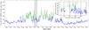 |
Fig. 1 RXTE All Sky Monitor lightcurve of Cyg X-1 rebinned to a resolution of 1 d for the two year period surrounding the observations. The times of our four analyzed observations are marked with the vertical lines. Color coding corresponds to spectral state classification as defined by Grinberg et al. (2013): the blue color represents hard state, while the green color represents the intermediate state data. The inset is zoomed in on the four observations, with a resolution of one data point per spacecraft orbit. |
The EPIC-pn data were reduced following standard Timing Mode data reduction steps with the Science Analysis Software (SAS) version 11.0.0 and the calibration of the Modified Timing Mode discussed in Appendix A. The increased soft X-ray emission of the transitional state of the source (Sect. 2.2) can potentially lead to pile-up in the center of the point spread function. Therefore we ignore the innermost three columns. As the new lower threshold energy limit of 2.8 keV might introduce possible transient effects (see Appendix A), we restrict the spectral analysis to energies above 4 keV. As seen in Fig. 2, the signal to noise ratio of the remaining data is exceptionally good. Throughout this paper we rebin all EPIC-pn data to S/N = 100, which resulted in a resolution of 40 eV at 6.4 keV, oversampling the detector response by a factor of ~4. All spectral fitting was performed with the Interactive Spectral Interpretation System (ISIS; Houck & Denicola 2000; Houck 2002; Noble & Nowak 2008).
A preliminary analysis of all four observations, which focused on the broad band spectrum and the Fe Kα line, was published in the thesis of Sonja Kreykenbohm née Fritz (Fritz 2008). Compared to that analysis, the results presented here utilize a significantly improved calibration strategy and more physical relativistic reflection models which have been developed since. We started this analysis with the publication of the observation with the least flux variability, Obs2 (Duro et al. 2011). Here, we focus on all four observations, and note the presence of higher flux variability in observations Obs1, Obs3, and Obs4 (see Fig. 3 and Table 1).
2.3. RXTE data
The broad emission feature (Fig. 2) makes it difficult to constrain the underlying continuum using the 4–10 keV XMM-Newton modified timing data alone. Therefore we use the much broader energy-range RXTE data that were taken simultaneously with all four XMM-Newton observations (observation IDs 90104-01-01-[00, 02], 90104-01-02-[00,01, 03], 90104-01-03-[00, 01] and 90104-04-1; Fig. 3). Its two well-calibrated instruments provide the coverage up to relatively high energies: the Proportional Counter Array (PCA; Jahoda et al. 2006), with its five large-area Proportional Counter Units (PCU), covers the 4–40 keV range (as used in this paper), while the High Energy X-ray Timing Experiment (HEXTE; Rothschild et al. 1998) provides us with 20–120 keV data.
The RXTE data were reduced with HEASOFT 6.11. From the PCA, we use the photons from the top anode layer of PCU 2 and filter out all data taken within 10 min of passages through the South Atlantic Anomaly and during the times of high particle background (Fürst et al. 2009). A systematic uncertainty of 0.5% was added in quadrature to the PCA data in order to account for uncertainties in the calibration. We applied the same temporal filtering criteria to the HEXTE data and added the spectra from both clusters together for the spectral analysis. The lightcurves in Fig. 3 show the typical RXTE orbital gaps and the flux in both instruments is following the trends seen in EPIC-pn data. HEXTE spectra were re-binned with S/N = 30, and no binning was performed on the PCA data.
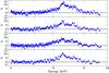 |
Fig. 2 Broad residuals at the iron line region (around 6.4 keV) in XMM-Newton EPIC-pn observations are uncovered by excluding the 5.5–8.0 keV region and modeling the remaining data with a cutoff power-law. There are evident absorption features in the line spectra that are due to Fe xxv (6.65 keV) and Fe xxvi (6.96 keV) in the local medium. |
2.4. Gainshift correction
As we discussed earlier (Duro et al. 2011), a single continuum model is not sufficient to describe the 4–120 keV data. Strong positive residuals remain in the broad Fe Kα line region and a mismatch in the RXTE and XMM-Newton residuals is apparent: the EPIC-pn line appear to be shifted to a slightly higher energy (Fig. 2 of Duro et al. 2011). This is also evident when adding a neutral 6.4 keV iron line to the data, which is required to be at 6.6 keV by the EPIC-pn data. This value is inconsistent with the Chandra measurements for the narrow feature in Cyg X-1, which clearly identify a spectral emission feature at 6.4 keV (e.g., Miller et al. 2002).
As discussed in more detail in Appendix B, this apparent difference between XMM-Newton and RXTE is due to Charge Transfer Efficiency (CTE) effects in the EPIC-pn instrument, a well-known effect that occurs in all X-ray CCDs: as the charge deposited at the impact point of a X-ray photon is moved to the border of the CCD and read out, some of the charge is lost to energy sinks (“traps”) in the silicon crystal. For low count rates the amount of charge lost is well-known as a function of the impact position of the photon. The standard analysis pipelines take the known value of the CTE into account when converting the measured charge back into a “pulse invariant” photon energy (see, e.g., Guainazzi et al. 2014; Pintore et al. 2014). When a bright source is observed, the photon rate can become high enough that the traps become filled in electrons. As a result, less charge is lost during the read out of the CCD than in normal observations and the charge arriving at the read out of the EPIC-pn CCD is larger than during normal operations. When converting this charge back to a photon energy in the SAS, the energy assigned to the event, Eobs, will be wrong. As discussed further in Appendix B, this erroneous energy assignment can be modeled as a linear gain shift, which can be parameterized with a model of the form  (1)where Eobs is the energy assigned to events in the SAS, Ereal is the real photon energy, s is the gain shift parameter and ΔE is a potential energy offset, which should be 0 keV for a purely CTE related gain shift. As we show in Appendix B, joint fitting of narrow line features from Fe xxv and Fe xxvi as seen in the Chandra and XMM-Newton data, as well as joint fitting of the spectral continuum as measured with the RXTE-PCA and EPIC-pn data, gives consistent values of the energy gain-shift s ~ 1.02 to a precision of ~2%, while the intercept ΔE is consistently at 0 keV. Applying this gain shift correction to the XMM data then achieves a consistent description of the XMM-Newton-pn and PCA data.
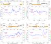 |
Fig. 3 Background subtracted lightcurves for all four observations. Bottom panels: XMM-Newton and RXTE lightcurves, binned to a resolution of 96 s. Top panels: INTEGRAL-ISGRI lightcurves, binned to a resolution of 40 s. The black continuous line shows science window averaged count rates, i.e., averages over the ~30 min long individual INTEGRAL pointings. Data used in the analysis, i.e., data with roughly the same count rate level as that measured during the XMM-Newton observations, are shown in orange. Gray data points are from time intervals not used. The same flux variation is evident in all four instruments. Note that Obs4 is the shortest observation. See Table 1. |
2.5. INTEGRAL data
In addition to the RXTE observations, we also obtained simultaneous INTEGRAL data (INTEGRAL; Winkler et al. 2003) during the XMM-Newton observations (see Table 1). We use data from the INTEGRAL Soft Gamma-Ray Imager (ISGRI; Lebrun et al. 2003) of the Imager on-Board the INTEGRAL Satellite (IBIS) coded mask instrument Ubertini et al. (2003) in the 20–500 keV range.
We reduced the data with OSA 9.2 following the standard reduction procedures (Goldwurm et al. 2003), and only used data where the source was within 14° of the center of the field of view of the IBIS detector. IBIS spectra were extracted in 64 energy channels. As the strictly simultaneous data have too short exposure times (texp ~ 12 ks) to achieve a reasonable quality for INTEGRAL data, we investigated different possibilities for co-adding of spectra.
Using data from a whole INTEGRAL revolution increases the exposure time to ~70 ks. However, the joint modeling with XMM-Newton and RXTE does not give a good description of the data. This is likely due to the variability of the source during the individual observations (Fig. 3), which are accompanied by changes in spectral shape during these longer INTEGRAL exposures. Note that we have found that Cyg X-1 can undergo spectral changes on time scales as short as about half an hour (Böck et al. 2011). The interpretation is supported by the fact that the use of two power-laws, one for EPIC-pn, PCA and HEXTE, and one for the full ISGRI exposure, results in slightly different photon indices, indicating that the spectra have a slightly different continuum shape.
To reduce the influence of this intrinsic source variability and at the same time to maximize the exposure time, we use spectral data from those periods within each INTEGRAL revolution, where the ISGRI flux levels are comparable to the ISGRI flux levels during the strictly simultaneous XMM-Newton observations (Fig. 3). This approach produces a good overall description of the spectrum.
As a cross check, in order to better assess the influence of INTEGRAL data we modeled the data of all instruments using all three approaches to INTEGRAL data. As expected given the ISGRI energy range, the parameters of the Fe Kα line, which is the focus of this paper, were not significantly influenced by small changes in the high energy continuum.
3. The Relativistically Broadened Fe Kα line
3.1. Continuum model
The raw data of EPIC-pn show the presence of a spectral emission feature at ~6.4 keV. To assess the feature we first model the spectrum excluding bins in the energy range from 5.5–8 keV with a single power-law, which is then applied to the complete 4–9.5 keV region. Figure 2 shows clear residuals in all four observations. As discussed earlier (Wilms et al. 2006a; Duro et al. 2011), the broad feature is a direct signature of two major effects: the Compton broadening in the strongly ionized reflector that smears out all other discrete features such as edges in the reflection spectrum and the Doppler and general relativistic effects that affect the photons of the intrinsically narrow Fe Kα line and that arise due to the proximity of the reflector to the black hole. Additionally, our observations were made during the orbital phase φorb ~ 0.8 so that a fraction of the photons is absorbed by the local medium (Hanke et al. 2009; Miškovičová et al. 2016). This produces the two absorption lines of Fe xxv and Fe xxvi which are superimposed on the broad emission line (see also Díaz Trigo et al. 2006 and references therein for a discussion of ionized absorbers). These lines need to be taken into account during the spectral modeling. We also generally assume an optically thick and geometrically thin accretion disk (Shakura & Sunyaev 1973; Novikov & Thorne 1973), i.e., a radius-dependent line emissivity per disk unit area that scales with r− ϵ.
Best fit parameters for a coronal model using a cutoff power-law and relativistic reflection.
Because of the complex reflection spectrum, modeling the spectrum by just ading a relativistic line to a continuum described by a power-law with an exponential cutoff does not result in a good description of the data. The reduced χ2 values of such fits vary from 1.44 to 2.17 if ϵ is left free, and are 4.61 and higher for fixed ϵ = 3. We therefore describe the data with a more physics based model, which properly takes into account reflection from an ionized disk. In order to do so, we use the reflionx model (e.g., Ross & Fabian 2005; Fabian & Ross 2010), which effectively models the main reflection features: the strongest line transitions, and the Compton reflection component between 20 and 40 keV, which is due to the Compton scattering in the disk. The model’s most important parameters are the Fe abundance and the ionization parameter, ξ, expressed in units of erg cm s-1.
Reflionx does not include the relativistic effects due to the emitting region’s proximity to the black hole. To take them into account, we convolve the reflection spectrum with the relativistic convolution model relconv (Dauser et al. 2010). The underlying spectral continuum is described by a cutoff power-law (note that the value of 300 keV that is assumed by reflionx is too high for the values inferred for Cyg X-1, which yield Efold ≤ 200 keV). We assume isotropic angular distribution of the fluorescence photons, which are due to the up-scattered photons coming from a hot corona (Svoboda et al. 2009). In addition, the soft excess is described with the multi temperature disk black body diskbb (Mitsuda et al. 1984), while the absorption lines of Fe xxv and Fe xxvi are described with Gaussian profiles, gabs. The narrow 6.4 keV emission line feature is described with a Gaussian model (egauss in ISIS). In all spectral models flux normalization constants, constant in ISIS, are given relative to PCA, differences in flux normalization between the instruments are modeled with instrument-dependent multiplicative constants. In summary, in ISIS notation the spectral model is  (2)
(2)
3.2. Continuum
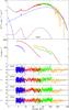 |
Fig. 4 Spectral modeling of the joint data. Top: unfolded XMM-Newton, RXTE and INTEGRAL data and best fit model components for the Corona geometry for Obs2. Blue line: continuum spectrum including the narrow iron Kα emission line and the black body. Purple line: relativistically smeared reflection component. Second panel: measured count rate spectra. The four lowest panels show the best fit residuals for observations Obs1–Obs4. EPIC-pn is blue, PCA is red, HEXTE is green and ISGRI is orange. |
Figure 4 shows that for all four observations the model describes the 4–500 keV energy spectrum well. The reduced χ2 varies from  (Obs4; 331 d.o.f.) to
  (Obs1, 393 d.o.f.), see Table 2. The normalization constants between the instruments are stable and well constrained.
The photon index shows little change between the observations, Γ ~ 1.6, with only Obs1 softening to Γ ~ 1.7. In this observation the source is brighter and the flux strongly variable for a significant part of this observation2 (Fig. 3), probably leading to the softening and the comparatively poor fits. This interpretation is consistent with the highest gain-shift value for Obs1 (sgainshift ~ 1.027) as the high source flux is able to saturate silicon traps faster, leading to a wrong CTE correction (see Appendix B). Excluding the period of increased flux and fitting Obs1 again, using a total of 8 ks of EPIC-pn observation with the corresponding HEXTE, PCA and same flux ISGRI data (Fig. 3), results in an excellent spectral model with  . The gain-shift slope decreases in value to
  , in better agreement with other observations, i.e., the CTE over-correction is less severe. The photon index hardens to
  confirmining the effect of the flare on the overall shape of the continuum that leads to the bad fit to the total Obs1.
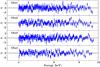 |
Fig. 5 Best fit XMM-Newton residuals for Corona geometry for observations Obs1–Obs4 for the fits of Fig. 4. No systematic variations are present. |
The folding energy, which reflects the electron temperature in the corona, is stable for all four observations around Efold ~ 170 keV. The study by Nowak et al. (2011) that uses hard-state broad band data of Suzaku and RXTE shows folding energy values that are consistent with our results (see also Wilms et al. 2006b).
A possible criticism of our model is that it does not fit well the data above 100 keV, where ISGRI is dominant (Fig. 4). As already discussed in Sect. 2.5, using only strictly simultaneous ISGRI data does not improve the results. We expect the broad band ISGRI data to mostly affect hard continuum parameters, especially the folding energy Efold. We can observe exactly this behavior in our data: repeating the modeling excluding the ISGRI data, the value Efold strongly increases and it is weakly constrained ( keV, Duro et al. 2011), while the remaining parameters do not change significantly.
Furthermore, it is clear that the underlying continuum affects the fit to the Fe Kα line in general. It is therefore important to see that the fit to the continuum does not produce any systematic variations in the residuals of the XMM-Newton data, which are critical for the extraction of line parameters. As Fig. 5 shows, no significant systematic variations can be observed.
3.3. Coronal geometry
3.3.1. Disk reflection with ϵ = 3
Having established that our continuum parameters are largely stable throughout all four observations, we now focus on the disk reflection. We start with modeling the disk reflection using the commonly used empirical emissivity profile ∝ r− ϵ with a standard value of ϵ = 3 (see, e.g., Fabian et al. 2012). Figure 4 and Model 1 in Table 2 show the resulting best fit residuals and values. The line profile indicates a high angular momentum of the black hole. All four observations point consistently towards a spin value of a> 0.9. In Fig. 7 we examine the correlation between the parameters with the largest impact on the shape of the Fe Kα line feature, i.e., spin, a, inclination, i, and emissivity index, ϵ. The third row of Fig. 7 shows correlations with models where ϵ was held fixed at ϵ = 3. They result in a high spin solution and an inclination that is consistent with measurements of ~27° (Orosz et al. 2011)3. These inferred spin values agree well with Gou et al. (2011), who obtain an extreme spin value for Cyg X-1, a ~ 0.9, by thermal continuum spectrum fitting, and with Fabian et al. (2012), who fit the reflection spectra. The Fe abundance is well constrained in all cases to a few times the solar value, consistent with results obtained previously.
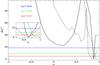 |
Fig. 6 χ2 behavior of the spin a for the broken power law emissivity disk profile (Model 3). All four observations have their best minima at a ~ 0.9. Obs1 is drawn with solid, Obs2 with dashed, Obs3 with dotted and Obs4 dot-dash-dotted line. The zoom-in figure shows the area around the minima, produced with very fine binning. Similar behavior is produced for the single power-law profile. |
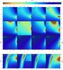 |
Fig. 7 Parameter correlations for the coronal model with a cutoff power-law and relativistic reflection with ϵ fixed at ϵ = 3 and as a free parameter (Models 1 and 2 in Table 2). First row: holding the inclination fixed at i = 27° results in one best fit solution for the emissivity index ϵ and spin a. Second row: for i let free, one more solution emerges. We chose the physical one as the best fit (see Sect. 3.3.2). Third row: ϵ = 3 is chosen to describe the correlation between i and a. Fourth row: interplay between ϵ and i. Shown are the χ2 significance contours for two parameters of interest based on Δχ2 = 2.30, 4.61 and 9.21, i.e., 68%, 90% and 99% confidence levels, with respect to the best fit case. |
3.3.2. Disk reflection with ϵ free
What happens if we leave both the emissivity profile index ϵ and the inclination i free? Such a setup produces a slightly better reduced χ2 then a fixed emissivity, ranging from 1.18 (331 d.o.f.) to 1.38 (392 d.o.f.; Model 2 in Table 2). In Obs2 and Obs3 the only solution found is for ϵ ~ 3 and spin a ~ 0.9, reproducing the result for fixed value of ϵ. This is not entirely true for the observations Obs1 and Obs4 in which the best fit solution produces retrograde spin values, a ≤ 0. A negative spin means that the ISCO is further away from the black hole, with RISCO ≥ 6rg. Coupled with the very dramatic increase in the emissivity profile index value ϵ ~ 10 (see Table 2), this results in an unphysical situation that is, at best, very difficult to explain. We note, however, that even for these two observations, we find acceptable fits for the combination of high a and low ϵ (see the second row on Fig. 7 for χ2 significance maps).
The shape of the line profile is in part determined by ϵ and i. The higher emissivity index ϵ for spinning black holes produces broader and more red-shifted profiles, as the irradiation is more concentrated on the inner parts of the accretion disk, while the decreasing inclination i shifts the blue wing in the reflection feature towards lower energies (see, e.g., Dauser et al. 2013). Thus, the emissivity profile index ϵ and the inclination i are somewhat correlated, as can be seen in the fourth row of Fig. 7. On the same figure we see that the inclination obtained in our fits is consistent with i ~ 27°. Fixing i at this value and re-fitting enables us to almost reproduce the results obtained for ϵ fixed at a value of 3. The best fit values for Model 2 are shown in Table 2.
3.3.3. Disk Reflection with a broken power-law for the emissivity profile
In order to improve the unrealistic combinations of low spin and high emissivity index obtained for a single power-law emissivity (Sect. 3.3.2), we employ a broken power-law emissivity profile to model the irradiation of the disk in a more realistic way. For example, a compact corona or an irradiation of the disk by a compact central source lying above the accretor produces a steep emissivity profile at the inner part of the disk, converging to r-3 at the outer regions (Fukumura & Kazanas 2007; Wilkins & Fabian 2011; Dauser et al. 2013). To describe this kind of behavior we describe the emissivity profile with a broken power law, where we fit the inner emissivity index, ϵin, and fix the emissivity for the outer disk to ϵout = 3. We constrain the break of the power-law to occur within 6rg from the black hole, as no steep emissivities are expected at larger radii (e.g., Dauser et al. 2013). Model 3 in Table 2 shows the best fit values for all four observations. The table reveals that  is similar or better than for the single power-law emissivity profile disk description (with one less degree of freedom). The best fit residuals are similar to the ones presented in Fig. 4 and are therefore not shown.
Compared to the single power-law emissivity description (Sect. 3.3.2), the most prominent change is the disappearance of the unphysical solutions for Obs1 and Obs4. For all four observations, only one spin solution with a ~ 0.9 is found, as clearly seen on Fig. 6 where we show the behavior of the goodness of the fit for different values of a. The zoom-in on the high spin region shows that the minima of χ2 are consistently at a ~ 0.9. Note that a similar behavior is achieved for the single power-law emissivity if we fix ϵ = 3. As already motivated above, the break in emissivity occurs close to the black hole as expected from calculations of more physical emissivity profiles (see, e.g., Dauser et al. 2013). Moreover, the inferred value of rbreak ~ 3.5rg is consistent with the break radius found by Fabian et al. (2012) for Cyg X-1. We find a very steep emissivity profile for small radii, 4 ≤ ϵin ≤ 10, implying that most of the reflected Fe Kα emission of Cyg X-1 comes from these inner regions. The outer parts are following the standard emissivity profile of a thin disk. This is evident in the fourth row of Fig. 8 where ϵ changes follow this description with the increasing distance from the black hole, expressed by the break radius rbreak.
We emphasize that Fig. 8 clearly shows that the high spin solution a ~ 0.9 is required as a best fit solution with respect to ϵ, rbreak, and i. This result is consistent for all four observations. The remaining parameter values are in agreement with the single power-law emissivity description.
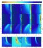 |
Fig. 8 Parameter correlations for fits with a broken power-law emissivity (Model 3 in Table 2). High spin is required in all situations. First row: emissivity index ϵ and spin a. Second row: break radius rbreak versus the spin a. Third row: inclination i with respect to the spin a. Fourth row: change in emissivity profile index ϵ with varying break radius rbreak. Shown are the χ2 significance contours for two parameters of interest based on Δχ2 = 2.30, 4.61, and 9.21, i.e., 68%, 90%, and 99% confidence, with respect to the best fit case. |
3.4. Lamp post geometry
Having shown that the best fit with a phenomenological model is achieved when using a broken power-law emissivity profile with a steep emissivity, we now turn to a physical model in which this emissivity behavior is naturally produced. The motivation for this model comes from the properties of the broad-band emission of Cyg X-1 that ranges from radio to X-rays (Markoff et al. 2005; Wilms et al. 2007; Rahoui et al. 2011, and references therein), and from the existence of a short time-scale radio-X-ray flux correlation in Cyg X-1 (Wilms et al. 2006b; Gleissner et al. 2004). X-ray emission from the source is probably due to synchrotron self-Comptonization in a relativistic jet that is launched along the rotational axis of the black hole (Markoff et al. 2005). The “lamp post” geometry assumes the hard X-ray radiation to be emitted from the base of this jet. As the source is very close to the black hole at a height of only a few rg, the light bending effects focus a large fraction of the photons onto the accretion disk, producing the observed reflection component. If the source is closer to the black hole, more photons illuminate the disk, and less are left over to produce the continuum component. With increasing height h, the opposite is true, creating the anti-correlation between the continuum and the reflection component, an effect that has already been observed in the AGN MCG−6-30-15 (Miniutti & Fabian 2004; Miniutti 2006).
For the spectral modeling we utilize the lamp post convolution model relconv_lp (Dauser et al. 2013). This model successfully incorporates the relativistic effects that are imprinted in the spectra due to the source’s proximity to the black hole. In the model, the height of the jet base, h, is a free parameter and expressed in units of rg. In the model, light bending and aberration effects lead to a “focusing” of the emission from the jet onto the disk and directly produce a very steep emissivity profile for the innermost few rg of the disk (see, e.g, Dauser et al. 2013, for examples of lamp post emissivity profiles). To fit the data, we use the continuum and the reflection model components as deduced from the coronal geometry in Sect. 3.1. These spectral components are expressed in the final model 4, which in ISIS notation, is given by 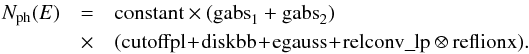 (3)The best fit solution residuals for all four observations are shown in Fig. 9. They are hardly distinguishable from the best fit solution using the coronal geometry (see Fig. 4). The values range from 1.23 to 1.46 (with the same degrees of freedom). Inspecting the XMM-Newton residuals does not reveal any systematic variations, similar to what was shown for the coronal geometry in Fig. 5. In all four observations we find extreme spin values (a ≥ 0.9). The jet height h remains at very low values, i.e., h ~ 3rg. The low height of the jet base indicates the presence of many primary photons irradiating the disk and can therefore explain the significant amount of reflection (Dauser et al. 2013). Although an anti-correlation between the jet height h and the inclination i seems to be present (see Fig. 10), low values for both parameters are required by the data. We note that the inclination i ≥ 30° is somewhat higher than for the coronal geometry. The second row of Fig. 10 shows that, irrespective of the inclination i, the data consistently require high values of the spin. Similarly, the h-a dependence in the top row of the Figure also demonstrates that a high spin value is required by the data. The remaining relevant parameters are consistent with the values obtained from the coronal geometry fits, i.e., Fe/Fe⊙ ~ 4, sgainshift ~ 1.02 and Efold ~ 170 keV.
As both geometric models lead to similar χ2 values and produce consistent parameter values, we conclude that from our data it is impossible to distinguish between the lamp post and the coronal geometry. Similar model comparisons were also performed for Cyg X-1 using Suzaku data (Nowak et al. 2011) as well as for the galactic black hole GX 339−4, for which Markoff et al. (2005) could show that their RXTE data are equally well described when using both accretion flow geometries (Markoff et al. 2005). Table 3 gives an overview of the best fit values for the lamp post model.
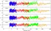 |
Fig. 9 Residuals for fits with the lamp post model for all four observations using XMM-Newton (blue), RXTE (PCA: red, HEXTE: green), and INTEGRAL (orange) data. |
4. Discussion
4.1. The spin of Cygnus X-1
Assuming that the inner edge of the accretion disk extends to the ISCO allows us to interpret the changes of the intrinsically narrow Fe Kα emission line as the relativistic effects that arise due to the closeness of the disk emission region to the black hole. Several previous investigations are in favor of this assumption. For example, Reis et al. (2010) have excluded truncation of the disk in the low-hard state of 9 stellar mass black holes (including Cyg X-1). We also refer to the recent study of Cyg X-1 by Miller et al. (2012), where the inner disk radius in hard state Suzaku data was also found to be relatively stable despite the changes in the power-law and the flux variations of the radio component. Miller et al. (2012) find the spin in the range 0.6 ≤ a ≤ 0.99, which agrees well with the very high spin of Cyg X-1 that we have derived here. Recent results coming from reflection fitting (Fabian et al. 2012), continuum fitting (Gou et al. 2011), or from both methods (Tomsick et al. 2014), strengthen the assumption and confirm the high spin of Cyg X-1.
Gou et al. (2011) analyzed soft state data from the Advanced Satellite for Cosmology and Astrophysics, RXTE, and Chandra using the continuum-fitting method (Zhang et al. 1997), finding a ~ 0.99. The results were examined by carrying out several tests (i.e., using different reflection models and a change in inclination angle and metallicity), all consistently showing a high spin value. These authors derived the emissivity profile index of the disk to be ϵ ~ 2.8, the convolution models kerrconv and kerrdisk (Brenneman & Reynolds 2006). The value agrees well with our broken-power-law emissivity profile model for the outer disk region (≥4rg) and with the low source height h ~ 3rg for the jet base in the lamp post model. Our models also require a high spin value for all physically meaningful values of the relevant parameters such as i, ϵ, h, and rbreak, in agreement with the continuum-fitting results.
Fabian et al. (2012) measured the spin by fitting reflection models to hard-state Suzaku data. Their result of  is based on fitting for an emissivity profile that goes as a broken-power law, in which the steep value of ϵ ≥ 6.8 is achieved for the innermost region of rbreak ≤ 5.1rg, while the outer disk takes the standard thin disk emissivity profile value of ϵ = 3. Fabian et al. (2012) note, however, that using a single power-law with ϵ = 3 does produce an extreme spin value as well. Using a single power-law emissivity profile we have previously derived a similarly high value (Duro et al. 2011).
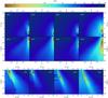 |
Fig. 10 Parameter correlations for the lamppost model (Model 4 in Table 3). Shown are the χ2 significance contours for the two parameters of interest. First row: jet base height h in units of GM/c2 versus the black hole spin a. Second row: inner disk inclination i expressed in degrees versus the spin a. The values clearly point towards a high spin value. Third row: inner disk inclination i versus the jet base height h. Shown are the χ2 significance contours for two parameters of interest based on Δχ2 = 2.30, 4.61, and 9.21, i.e., 68%, 90%, and 99% confidence, with respect to the best fit case. |
We are able to reproduce this result in all four observations for the extended energy range used here (Sect. 3.3.1). The best description, however, is achieved by using a broken power-law for the emissivity profile. The spin is a ~ 0.9, while the break radius is at ~4rg with the outer region’s emissivity index, ϵout fixed at 3. The profile is very steep for observations Obs1 and Obs4, ϵin ~ 10, for the inner disk region. It less well constrained than in Obs2 and Obs3, possibly owing to the flares and the short exposure time in Obs1 and Obs4. The good description of the data by the broken power-law for the emissivity profile is expected, specifically for compact emission sources located near the central object (Dauser et al. 2013), as strong gravitational effects require a steep profile for the inner disk region (Wilkins & Fabian 2011).
Best fit parameters for the lamp post model for all four observations (Model 4).
In their analysis of the combined data of the 1–300 keV simultaneous Nuclear Spectroscopic Telescope Array (NuSTAR) and Suzaku data of Cyg X-1 in the soft spectral state, Tomsick et al. (2014) model the spectrum using both the reflection and the continuum fitting methods. The broad energy coverage of these data enables them to constrain the parameters of the thermal disk emission, the continuum, and the reflection emission. They find the iron line to be very broad and asymmetric with an extended red wing, i.e., to show clear signs of relativistic influence on the intrinsic emission. The relativistic reflection model components applied were the same as in our analysis (relconv, relconv_lp), but they modified the intrinsic reflection model reflionx to accept higher ionization levels than in its standard version used here.
An exploration of different models and parameter values showed that the spin value from the accepted model fits was a> 0.83 (Tomsick et al. 2014), which is consistent with our results. The emissivity profile yields a high ϵ value for the inner disk region, as also seen in our work. Interestingly, the inclination inferred by Tomsick et al. (2014) implies a higher value of the inclination than Orosz et al. (2011) found using optical spectroscopy. We will return to the discussion of the inclination further below (Sect. 4.3).
We note that some earlier papers have claimed low spin values of a ~ 0 for Cyg X-1 (e.g., Miller et al. 2002, 2009), which are clearly inconsistent with our inferred spin for Cyg X-1. Common to these earlier models was that in addition to lacking precise measurements of the distance, inclination, and mass of Cyg X-1. They also did not have the high energy coverage (≥10 keV) that is crucial in order to constrain the underlying continuum and reflection features properly (Ng et al. 2010). The current moderate abundance of the data with high enough S/N and broad energy coverage, and the availability of more complex, yet more physically realistic models, have helped to remove the inconsistency and achieve the agreement on the high spin of Cyg X-1. This is precisely what is consistently concluded by the most recent results from the disk-dominated state (Gou et al. 2011; Tomsick et al. 2014), the hard intermediate state (this work), and the hard state (Fabian et al. 2012; Miller et al. 2012).
4.2. The accretion geometry of Cygnus X-1
It is difficult to distinguish between different proposed accretion geometries. We examined the coronal geometry where we described the disk emissivity profile with a single or broken power-law. As noted before, both provide a good descriptions of the data, with a preference for a break in the emissivity profile. Model fits with the lamp post geometry lead to an equally good description of the data. This similarity may point in the direction of a close connection between the corona residing close to the black hole and the material being collimated into a jet as suggested by Markoff et al. (2005), building on earlier work on the accretion flow structure by, for example, Nowak et al. (2002) and Merloni & Fabian (2002). In this model, hard photons are created in the jet base by synchrotron and synchrotron self-Compton up-scattering. Markoff et al. (2005) compare the model with thermal corona models, concluding that despite the high statistics of RXTE spectra it is not possible to distinguish between the jet model and thermal Comptonization. This result was later confirmed by Nowak et al. (2011) with even higher signal to noise data and with a better energy coverage.
Miller et al. (2012) propose several interesting properties that may serve to put more constraints on the geometry of the system. Based on twenty Suzaku hard state Cyg X-1 observations, the correlation between the radio flux and the inner accretion disk temperature, as well as the correlation with the reflected X-ray flux, suggest strong disk-jet coupling. Using these findings, Miller et al. (2012) propose a system where the corona/jet base is produced of the disk material that is lifted by the magnetic forces, and (partly) accelerated by the pressure of the reflected radiation (for more details, see Miller et al. 2012). Such a geometry approximately identifies the jet base with the corona, which could explain the similarities we obtained from the coronal and the lamp post geometry. Ideally, this could be further tested by simultaneous EPIC-pn and radio observations.
It is worthwhile to note that in the lamp post geometry, an Fe Kα line that is very broad is already telling us that the black hole is highly spinning and that the continuum source is compact and is close to the black hole (i.e., with low height h). This is due to the nature of the emission source, as concluded by Dauser et al. (2013). An elongated (and/or accelerated) jet produces spectral lines that are narrow, and which are independent of the black hole spin a. A similar line shape is achieved with a low spin and a compact emission source, making the distinction from a high-spin elongated jet case impossible. Only the combination of a high spin and a low and compact jet produces a broad line that can be distinguished from the other three cases (see Fig. 10 of Dauser et al. 2013).
4.3. The inclination of the inner disk
In all our fits the inferred inclination is close to i ~ 30°. This agrees well with many previous studies that consider different approaches to constrain the inclination of the Cyg X-1 system. The lack of a significant dependence of the Hα emission strength on the orbital phase φ has led Sowers et al. (1998) to constrain the inclination to i ≤ 55°. Likewise, the lack of a two-sided jet detection suggested a low inclination of the system (Stirling et al. 2001). The most probable/realistic evolutionary models of Ziółkowski (2005) result in an inclination in the range of 28° ≤ i ≤ 38°. More recently, based on optical measurements, Orosz et al. (2011) adopt a model with eccentric orbit and asynchronous rotation at periastron which produces an inclination of , and  from their second best model assuming synchronous rotation. Comparing these measurements of the system’s inclination with our measurement of the inclination of the disk close to the black hole shows that in our intermediate/hard state observations the inner disk and the orbital angular momentum are in agreement. If we assume that the inner disk is aligned with the black hole’s spin, then we find that the spin axis and the orbital momentum vector are aligned, as predicted, for example, by Bardeen & Petterson (1975) and King et al. (2005).
There is, however, some discrepancy between our result and the high precision inclination measurement made by Tomsick et al. (2014) who used simultaneous NuSTAR and Suzaku observations in the soft state. Their fits require an inclination that is at least 13° higher than the optically derived value of Orosz et al. (2011) while our data agree with the optical inclination.
One possibility to explain this discrepancy is a systematic error in the modeling approach. For example, we have shown in Fig. 7 that the steepness of the emissivity profile, ϵ, is strongly correlated with the inclination. Given the high quality of the NuSTAR data, however, the systematic error is likely to be much smaller than the discrepancy between the best fit values for the inclination. In addition, we would also expect the spin parameters to be different between the NuSTAR fits and our fits if a systematic error was involed. This is not the case, and therefore it is unlikely that systematic effects are to blame for the difference in inclination.
If it is not due to systematics, then the difference in measured inclinations must be a real physical effect. We first re-emphasize that the inclination measured from the Fe Kα line is the inclination of the (thin) accretion disk close to the black hole, while the inclination measured optically is the inclination of the system as a whole. A difference between the inclination determined from the Fe Kα line and the optical inclination then implies that the accretion disk may be warped in its inner regions. While it is reasonable to assume that the angular momentum vector of the accretion disk is aligned with the orbital angular momentum (i.e., the angular momentum of the accreted material), the timescale for accretion to align the black hole with the orbital angular momentum is 106–108 years (Steiner & McClintock 2012 and references therein). A full alignment between the disk and the orbit is therefore not expected for a comparably young High Mass X-ray Binary. Furthermore, starting with the pioneering work of Bardeen & Petterson (1975), many authors have shown that it is possible to produce a warp in the inner regions of the disk (e.g., Pringle 1996; Fragile 2009).
Warped accretion disks often lead to long-term quasi-periodic modulations which are observable in the X-ray lightcurves (Clarkson et al. 2003a), such as the 35 d cycle of Her X-1 (e.g., Staubert et al. 2009) or the variable long-term period in SMC X-1 (Clarkson et al. 2003b; Trowbridge et al. 2007). The well-known 150 d or 300 d quasi-periodicity of Cyg X-1 has been associated with a similar warp (Priedhorsky et al. 1983; Kemp et al. 1983, 1987; Brocksopp et al. 1999; Zdziarski et al. 2002, 2011; Benlloch et al. 2004, and references therein).
If the warp is due to some kind of radiative instability (Pringle 1996; Maloney et al. 1998; Clarkson et al. 2003b) then the inclination of the inner disk produced by this warp could depend on the source luminosity and/or the mass accretion rate. For example, as recently shown by McKinney et al. (2013), thick disks with jets are much more stable against warping than thin disks. According to these simulations, the inner disk is therefore aligned with the orbital angular momentum during the hard state and the measured inclination should be the same for the binary orbit as for the inner accretion disk. During the soft state, the inner disk is warped and the measured disk and orbital inclinations can disagree. One can speculate whether such a behavior is the reason for the difference of our results with the soft state observations of Tomsick et al. (2014).
As a caveat, however, and somewhat contrary to this hypothesis, we note that the 150 d period in Cyg X-1 is strongest during the hard state and not present during the soft state (Benlloch et al. 2004; Zdziarski et al. 2011). As discussed by Zdziarski et al. (2011), if this period is due to a warped disk, then the cause for the warp is probably not entirely due to irradiation effects. However, it might also be that the 150 d period is unrelated to the disk, and, for example, due to jet precession without associated disk precession.
A further study of this behavior would require a detailed comparison of the Fe Kα line profiles measured in different states of Cyg X-1. A preliminary comparison of the NuSTAR profiles of Tomsick et al. (2014) and our XMM profiles shows line profiles to be different, independent of the continuum model used. The blue wing of the NuSTAR line, which is most relevant for the determination of the inclination, is more pronounced in these data, as expected for a higher inclination. More recent hard state measurements with NuSTAR have a less pronounced blue wing, which is more in line with the XMM data presented here. A further comparison of all available high signal-to-noise ratio line profiles of Cyg X-1 is needed for a more quantitative description. Such a comparison, however, is outside of the scope of this work.
5. Summary and conclusion
In this work we presented the analysis of four Cyg X-1 broadband (4–500 keV) observations taken simultaneously with XMM-Newton, RXTE, and INTEGRAL. Our focus was on the broad Fe Kα line, which is an excellent tool for probing the strong gravity regime of the black hole. We show that the black hole in Cyg X-1 is rapidly rotating, while the system’s inclination is at i ~ 30°. The XMM-Newton EPIC-pn was operated in the Modified Timing Mode that provided us with an excellent S/N coverage at the iron line region around 6.4 keV. The broad band data of RXTE-PCA, RXTE-HEXTE and INTEGRAL-ISGRI were used to constrain the underlying continuum, which is a crucial step as the shape and the strength of the Fe Kα line depend strongly on the correct modeling of the continuum. Our conclusions are the following:
-
1.
Cyg X-1 is found in the hard intermediate state.The cutoff power law describes the continuum well, although aweak black body component with TBB of a few hundred eV is additionally needed to describe the soft part of the spectra. The cutoff energy is at Efold ~ 170 keV.
-
2.
We find a broad Fe Kα line spectral feature at E ~ 6.4 keV. The broadening is due to the relativistic effects arising in the vicinity of the black hole, and the Doppler broadening due to the ionized reflector. The line cannot be described well with the simple modern relativistic Fe line models like relline. A full reflection model (reflionx) convolved with a relativistic model (relconv) is needed to describe the reflection spectra.
-
3.
The standard accretion flow geometry for black hole binaries in which the thermal electrons up-scatter the soft disk photons, describes the spectra well in all four observations. The result is a very rapidly spinning black hole with a ~ 0.9 and an inclination of the inner, moderately ionized disk of i ~ 30°. A broken power-law for the emissivity profile of the disk provides best fits (Models 2 and 3), although similar results can be achieved with a Newtonian power-law emissivity profile of r-3 (Model 1).
-
4.
The lamp post geometry, in which the base of the jet is the source for the continuum and the irradiation of the accretion disk, improves the fit slightly. For all four observations, the black hole parameters are similar to the coronal modeling in all four observations (Model 4). The distance of the jet base to the event horizon is small, resulting in a efficient irradiation of the inner accretion disk which produces significant disk reflection.
The high signal to noise ratio of our data allows us to strongly constrain the spin of the black hole. We demonstrated that the spin values inferred from our four observations are consistent, thus reducing the probability that our result is accidental. In addition, our result for the spin is also consistent with spin measurements found from line fitting with other instruments, such as Suzaku/NuSTAR, and with measurements performed during different source states. The line fitting method therefore gives consistent results irrespective of the accretion flow geometry. Our result is also consistent with the value obtained from continuum fitting, i.e., with a completely independent ansatz.
The next step in the endeavour of understanding Cyg X-1 is to find more ways to constrain the different accretion flow geometries, which cannot be distinguished from spectral fitting alone. The difference in the inner disk inclinations between the recent soft state Suzaku/NuSTAR measurement of Tomsick et al. (2014) and our results can be interpreted as an indication for a direct change in accretion geometry that has to be followed up by a more comprehensive survey of the Fe Kα line shapes in Cyg X-1. Together with improvements in the available physical models we hope that further constraints on the accretion flow geometry in this crucial system will soon be obtained.
Negative spin values mean that the angular momenta of the black hole and the disk are anti-parallel.
An increase of ~40%; compare to the stable Obs2, the less variable Obs3, and Obs4 that only has a short flare.
If only the non-flaring part of Obs1 is considered, the best fit is also consistent with this value of the inclination.
Using the newer version SASv11 does not improve calibration on observations used in this paper. The gain-shift correction in the model is still necessary to get a reasonable fit. See Pintore et al. (2014) and XMM-CAL-SRN-0083.
Acknowledgments
We thank Norbert Schartel and the XMM-Newton operations team for agreeing to perform observations in a new and untested mode, and Maria Díaz-Trigo for many useful discussions on CTE and pile up effects in the EPIC-pn camera. This work was partly supported by the European Commission under contract ITN 215212 “Black Hole Universe” and by the Bundesministerium für Wirtschaft und Technologie under Deutsches Zentrum für Luft- und Raumfahrt grants 50 OR 0701, 50 OR 1007, and 50 OR 1113. Further support for this work was provided by NASA through the Smithsonian Astrophysical Observatory (SAO) contract SV3-73016 to MIT for Support of the Chandra X-Ray Center (CXC) and Science Instruments. CXC is operated by SAO for and on behalf of NASA under contract NAS8-03060. JAT acknowledges partial support from NASA Astrophysics Data Analysis Program grant NNX13AE98G. We acknowledge the support by the DFG Cluster of Excellence “Origin and Structure of the Universe”. We are grateful for the support of M. Cadolle Bel through the Computational Center for Particle and Astrophysics (C2PAP). J.R. acknowledges funding support from the French National Research Agency, CHAOS project ANR-12-BS05-0009 (http://www.chaos-project.fr). This research has made use of ISIS functions provided by ECAP/Remeis observatory and MIT (http://www.sternwarte.uni-erlangen.de/isis/). We thank John E. Davis for development of the SLXfig package that was used to create the figures throughout this paper and Sasha Tchekhovskoy for useful discussions on accretion disk warping. This paper is based on observations obtained with XMM-Newton, an ESA science mission with instruments and contributions directly funded by ESA member states and NASA.
References
- Arnaud, K. A. 1996, in Astronomical Data Analysis Software and Systems V, eds. J. H. Jacoby, & J. Barnes, ASP Conf. Ser., 101, 7 [Google Scholar]
- Bałucińska-Church, M., Church, M. J., Charles, P. A., et al. 2000, MNRAS, 311, 861 [NASA ADS] [CrossRef] [Google Scholar]
- Bardeen, J. M., & Petterson, J. A. 1975, ApJ, 195, L65 [NASA ADS] [CrossRef] [Google Scholar]
- Benlloch, S., Pottschmidt, K., Wilms, J., et al. 2004, in X-ray Timing 2003: Rossi and Beyond, eds. P. Kaaret, F. K. Lamb, & J. H. Swank, Am. Inst. Phys. Conf. Ser. 714, 61 [Google Scholar]
- Böck, M., Grinberg, V., Pottschmidt, K., et al. 2011, A&A, 533, A8 [NASA ADS] [CrossRef] [EDP Sciences] [Google Scholar]
- Bolton, C. T. 1972, Nature, 235, 271 [NASA ADS] [CrossRef] [Google Scholar]
- Bowyer, S., Byram, E. T., Chubb, T. A., & Friedman, H. 1965, Science, 147, 394 [NASA ADS] [CrossRef] [Google Scholar]
- Brenneman, L. W., & Reynolds, C. S. 2006, ApJ, 652, 1028 [NASA ADS] [CrossRef] [Google Scholar]
- Brocksopp, C., Fender, R. P., Larionov, V., et al. 1999, MNRAS, 309, 1063 [NASA ADS] [CrossRef] [Google Scholar]
- Cadolle Bel, M., Sizun, P., Goldwurm, A., et al. 2006, A&A, 446, 591 [NASA ADS] [CrossRef] [EDP Sciences] [Google Scholar]
- Clarkson, W. I., Charles, P. A., Coe, M. J., & Laycock, S. 2003a, MNRAS, 343, 1213 [NASA ADS] [CrossRef] [Google Scholar]
- Clarkson, W. I., Charles, P. A., Coe, M. J., et al. 2003b, MNRAS, 339, 447 [NASA ADS] [CrossRef] [Google Scholar]
- Corbel, S., Fender, R. P., Tzioumis, A. K., et al. 2000, A&A, 359, 251 [NASA ADS] [Google Scholar]
- Dauser, T., Wilms, J., Reynolds, C. S., & Brenneman, L. W. 2010, MNRAS, 409, 1534 [NASA ADS] [CrossRef] [Google Scholar]
- Dauser, T., Svoboda, J., Schartel, N., et al. 2012, MNRAS, 422, 1914 [NASA ADS] [CrossRef] [Google Scholar]
- Dauser, T., Garcia, J., Wilms, J., et al. 2013, MNRAS, 430, 1694 [NASA ADS] [CrossRef] [Google Scholar]
- Díaz Trigo, M., Parmar, A., Miller, J. M., & Kuulkers, E. 2006, Astron. Nachr., 327, 1008 [NASA ADS] [CrossRef] [Google Scholar]
- Dovčiak, M., Karas, V., & Yaqoob, T. 2004, ApJS, 153, 205 [NASA ADS] [CrossRef] [Google Scholar]
- Duro, R., Dauser, T., Wilms, J., et al. 2011, A&A, 533, L3 [NASA ADS] [CrossRef] [EDP Sciences] [Google Scholar]
- Fabian, A. C., & Ross, R. R. 2010, Space Sci. Rev., 157, 167 [NASA ADS] [CrossRef] [Google Scholar]
- Fabian, A. C., Rees, M. J., Stella, L., & White, N. E. 1989, MNRAS, 238, 729 [NASA ADS] [CrossRef] [Google Scholar]
- Fabian, A. C., Zoghbi, A., Ross, R. R., et al. 2009, Nature, 459, 540 [NASA ADS] [CrossRef] [PubMed] [Google Scholar]
- Fabian, A. C., Wilkins, D. R., Miller, J. M., et al. 2012, MNRAS, 424, 217 [NASA ADS] [CrossRef] [Google Scholar]
- Fragile, P. C. 2009, ApJ, 706, L246 [NASA ADS] [CrossRef] [Google Scholar]
- Friend, D. B., & Castor, J. I. 1982, ApJ, 261, 293 [NASA ADS] [CrossRef] [Google Scholar]
- Fritz, S. 2008, Dissertation, Eberhard Karls Universität Tübingen [Google Scholar]
- Fukumura, K., & Kazanas, D. 2007, ApJ, 664, 14 [NASA ADS] [CrossRef] [Google Scholar]
- Fürst, F., Wilms, J., Rothschild, R. E., et al. 2009, Earth Plan. Sci. Let., 281, 125 [Google Scholar]
- Gies, D. R., & Bolton, C. T. 1986, ApJ, 304, 389 [NASA ADS] [CrossRef] [Google Scholar]
- Gleissner, T., Wilms, J., Pooley, G. G., et al. 2004, A&A, 425, 1061 [NASA ADS] [CrossRef] [EDP Sciences] [Google Scholar]
- Goldwurm, A., David, P., Foschini, L., et al. 2003, A&A, 411, L223 [NASA ADS] [CrossRef] [EDP Sciences] [Google Scholar]
- Gou, L., McClintock, J. E., Reid, M. J., et al. 2011, ApJ, 742, 85 [NASA ADS] [CrossRef] [Google Scholar]
- Gou, L., McClintock, J. E., Remillard, R., et al. 2014, ApJ, 790, 29 [NASA ADS] [CrossRef] [Google Scholar]
- Grinberg, V., Hell, N., Pottschmidt, K., et al. 2013, A&A, 554, A88 [NASA ADS] [CrossRef] [EDP Sciences] [Google Scholar]
- Grinberg, V., Pottschmidt, K., Böck, M., et al. 2014, A&A, 565, A1 [NASA ADS] [CrossRef] [EDP Sciences] [Google Scholar]
- Grinberg, V., Leutenegger, M. A., Hell, N., et al. 2015, A&A, 576, A117 [NASA ADS] [CrossRef] [EDP Sciences] [Google Scholar]
- Guainazzi, M., Kirsch, M. G. F., Haberl., F., et al. 2014, XMM-Newton Calibration Technical Note 83, XMM-SOC-CAL-TN-0083, available online at http://xmm2.esac.esa.int/docs/documents/CAL-TN-0083.pdf [Google Scholar]
- Hanke, M., Wilms, J., Nowak, M. A., et al. 2009, ApJ, 690, 330 [NASA ADS] [CrossRef] [Google Scholar]
- Hannikainen, D. C., Hunstead, R. W., Campbell-Wilson, D., & Sood, R. K. 1998, A&A, 337, 460 [NASA ADS] [Google Scholar]
- Houck, J. C. 2002, in High Resolution X-ray Spectroscopy with XMM-Newton and Chandra, ed. G. Branduardi-Raymont (Dorking, UK: Mullard Space Science Laboratory) [Google Scholar]
- Houck, J. C., & Denicola, L. A. 2000, in Astronomical Data Analysis Software and Systems IX, eds. N. Manset, C. Veillet, & D. Crabtree, ASP Conf. Ser., 216, 591 [Google Scholar]
- Jahoda, K., Markwardt, C. B., Radeva, Y., et al. 2006, ApJS, 163, 401 [NASA ADS] [CrossRef] [Google Scholar]
- Jourdain, E., Roques, J. P., Chauvin, M., & Clark, D. J. 2012, ApJ, 761, 27 [NASA ADS] [CrossRef] [Google Scholar]
- Kemp, J. C., Barbour, M. S., Henson, G. D., et al. 1983, ApJ, 271, L65 [NASA ADS] [CrossRef] [Google Scholar]
- Kemp, J. C., Karitskaya, E. A., Kumsiashvili, M. I., et al. 1987, Sov. Astron., 31, 170 [NASA ADS] [Google Scholar]
- Kendziorra, E., Bihler, E., Grubmiller, W., et al. 1997, in EUV, X-Ray, and Gamma-Ray Instrumentation for Astronomy VIII, eds. O. H. Siegmund, & M. A. Gummin, SPIE Conf. Ser., 3114, 155 [Google Scholar]
- Kendziorra, E., Wilms, J., Haberl, F., et al. 2004, in UV and Gamma-Ray Space Telescope Systems, eds. G. Hasinger, & M. J. L. Turner, SPIE Conf. Ser., 5488 613 [Google Scholar]
- King, A. R., Lubow, S. H., Ogilvie, G. I., & Pringle, J. E. 2005, MNRAS, 363, 49 [NASA ADS] [CrossRef] [Google Scholar]
- Laor, A. 1991, ApJ, 376, 90 [NASA ADS] [CrossRef] [Google Scholar]
- Laurent, P., Rodriguez, J., Wilms, J., et al. 2011, Science, 332, 438 [NASA ADS] [CrossRef] [PubMed] [Google Scholar]
- Lebrun, F., Leray, J. P., Lavocat, P., et al. 2003, A&A, 411, L141 [NASA ADS] [CrossRef] [EDP Sciences] [Google Scholar]
- Li, L.-X., Zimmerman, E. R., Narayan, R., & McClintock, J. E. 2005, ApJS, 157, 335 [NASA ADS] [CrossRef] [Google Scholar]
- Maloney, P. R., Begelman, M. C., & Nowak, M. A. 1998, ApJ, 504, 77 [NASA ADS] [CrossRef] [Google Scholar]
- Malzac, J., Belmont, R., & Fabian, A. C. 2009, MNRAS, 400, 1512 [NASA ADS] [CrossRef] [Google Scholar]
- Markoff, S., Nowak, M. A., & Wilms, J. 2005, ApJ, 635, 1203 [NASA ADS] [CrossRef] [Google Scholar]
- Martocchia, A., & Matt, G. 1996, MNRAS, 282, L53 [NASA ADS] [CrossRef] [Google Scholar]
- McConnell, M., Forrest, D., Ryan, J., et al. 1994, ApJ, 424, 933 [NASA ADS] [CrossRef] [Google Scholar]
- McConnell, M. L., Ryan, J. M., Collmar, W., et al. 2000, ApJ, 543, 928 [NASA ADS] [CrossRef] [Google Scholar]
- McKinney, J. C., Tchekhovskoy, A., & Blandford, R. D. 2013, Science, 339, 49 [NASA ADS] [CrossRef] [PubMed] [Google Scholar]
- Merloni, A., & Fabian, A. C. 2002, MNRAS, 332, 165 [NASA ADS] [CrossRef] [Google Scholar]
- Miller, J. M. 2007, ARA&A, 45, 441 [NASA ADS] [CrossRef] [Google Scholar]
- Miller, J. M., Fabian, A. C., Wijnands, R., et al. 2002, ApJ, 578, 348 [NASA ADS] [CrossRef] [Google Scholar]
- Miller, J. M., Reynolds, C. S., Fabian, A. C., Miniutti, G., & Gallo, L. C. 2009, ApJ, 697, 900 [NASA ADS] [CrossRef] [Google Scholar]
- Miller, J. M., Pooley, G. G., Fabian, A. C., et al. 2012, ApJ, 757, 11 [NASA ADS] [CrossRef] [Google Scholar]
- Miniutti, G. 2006, Astron. Nachr., 327, 969 [NASA ADS] [CrossRef] [Google Scholar]
- Miniutti, G., & Fabian, A. C. 2004, MNRAS, 349, 1435 [NASA ADS] [CrossRef] [Google Scholar]
- Mitsuda, K., Inoue, H., Koyama, K., et al. 1984, PASJ, 36, 741 [NASA ADS] [Google Scholar]
- Miškovičová, I., Hell, N., Hanke, M., et al. 2016, A&A, submitted [Google Scholar]
- Murdin, P., & Webster, B. L. 1971, Nature, 233, 110 [NASA ADS] [CrossRef] [Google Scholar]
- Ng, C., Díaz Trigo, M., Cadolle Bel, M., & Migliari, S. 2010, A&A, 522, A96 [NASA ADS] [CrossRef] [EDP Sciences] [Google Scholar]
- Noble, M. S., & Nowak, M. A. 2008, PASP, 120, 821 [NASA ADS] [CrossRef] [Google Scholar]
- Novikov, I. D., & Thorne, K. S. 1973, in Black Holes (Les Astres Occlus), eds. C. Dewitt, & B. S. Dewitt, 343 [Google Scholar]
- Nowak, M. A., Wilms, J., & Dove, J. B. 2002, MNRAS, 332, 856 [NASA ADS] [CrossRef] [Google Scholar]
- Nowak, M. A., Hanke, M., Trowbridge, S. N., et al. 2011, ApJ, 728, 13 [NASA ADS] [CrossRef] [Google Scholar]
- Orosz, J. A., McClintock, J. E., Aufdenberg, J. P., et al. 2011, ApJ, 742, 84 [NASA ADS] [CrossRef] [Google Scholar]
- Pintore, F., Sanna, A., Di Salvo, T., et al. 2014, MNRAS, 445, 3745 [NASA ADS] [CrossRef] [Google Scholar]
- Pottschmidt, K., Wilms, J., Nowak, M. A., et al. 2003, A&A, 407, 1039 [NASA ADS] [CrossRef] [EDP Sciences] [Google Scholar]
- Priedhorsky, W. C., Terrell, J., & Holt, S. S. 1983, ApJ, 270, 233 [NASA ADS] [CrossRef] [Google Scholar]
- Pringle, J. E. 1996, MNRAS, 281, 357 [NASA ADS] [Google Scholar]
- Rahoui, F., Lee, J. C., Heinz, S., et al. 2011, ApJ, 736, 63 [NASA ADS] [CrossRef] [Google Scholar]
- Reis, R. C., Fabian, A. C., Ross, R. R., & Miller, J. M. 2009, MNRAS, 395, 1257 [NASA ADS] [CrossRef] [Google Scholar]
- Reis, R. C., Fabian, A. C., & Miller, J. M. 2010, MNRAS, 402, 836 [NASA ADS] [CrossRef] [Google Scholar]
- Reid, M. J., McClintock, J. E., Narayan, R., et al. 2011, ApJ, 742, 83 [NASA ADS] [CrossRef] [Google Scholar]
- Reynolds, C. S., & Fabian, A. C. 2008, ApJ, 675, 1048 [NASA ADS] [CrossRef] [Google Scholar]
- Reynolds, C. S., & Nowak, M. A. 2003, Phys. Rep., 377, 389 [NASA ADS] [CrossRef] [Google Scholar]
- Ross, R. R., & Fabian, A. C. 2005, MNRAS, 358, 211 [Google Scholar]
- Rothschild, R. E., Blanco, P. R., Gruber, D. E., et al. 1998, ApJ, 496, 538 [NASA ADS] [CrossRef] [Google Scholar]
- Shakura, N. I., & Sunyaev, R. A. 1973, A&A, 24, 337 [NASA ADS] [Google Scholar]
- Sowers, J. W., Gies, D. R., Bagnuolo, W. G., et al. 1998, ApJ, 506, 424 [NASA ADS] [CrossRef] [Google Scholar]
- Staubert, R., Klochkov, D., Postnov, K., et al. 2009, A&A, 494, 1025 [NASA ADS] [CrossRef] [EDP Sciences] [Google Scholar]
- Steiner, J. F., & McClintock, J. E. 2012, ApJ, 745, 136 [NASA ADS] [CrossRef] [Google Scholar]
- Stirling, A. M., Spencer, R. E., de la Force, C. J., et al. 2001, MNRAS, 327, 1273 [NASA ADS] [CrossRef] [Google Scholar]
- Strüder, L., Briel, U., Dennerl, K., et al. 2001, A&A, 365, L18 [NASA ADS] [CrossRef] [EDP Sciences] [Google Scholar]
- Sunyaev, R.A., & Trümper, J. 1979, Nature, 279, 506 [NASA ADS] [CrossRef] [Google Scholar]
- Svoboda, J., Dovčiak, M., Goosmann, R., & Karas, V. 2009, A&A, 507, 1 [NASA ADS] [CrossRef] [EDP Sciences] [Google Scholar]
- Tanaka, Y., Nandra, K., Fabian, A. C., et al. 1995, Nature, 375, 659 [NASA ADS] [CrossRef] [Google Scholar]
- Thorne, K. S. 1974, ApJ, 191, 507 [Google Scholar]
- Tomsick, J. A., Nowak, M. A., Parker, M., et al. 2014, ApJ, 780, 78 [NASA ADS] [CrossRef] [Google Scholar]
- Trowbridge, S., Nowak, M. A., & Wilms, J. 2007, ApJ, 670, 624 [NASA ADS] [CrossRef] [Google Scholar]
- Ubertini, P., Lebrun, F., Di Cocco, G., et al. 2003, A&A, 411, L131 [NASA ADS] [CrossRef] [EDP Sciences] [Google Scholar]
- Webster, B. L., & Murdin, P. 1972, Nature, 235, 37 [NASA ADS] [CrossRef] [Google Scholar]
- Wilkins, D. R., & Fabian, A. C. 2011, MNRAS, 414, 1269 [NASA ADS] [CrossRef] [Google Scholar]
- Wilms, J., Kendziorra, E., Nowak, M. A., et al. 2006a, in The X-ray Universe 2005, ESA SP-604, 217 [Google Scholar]
- Wilms, J., Nowak, M. A., Pottschmidt, K., Pooley, G. G., & Fritz, S. 2006b, A&A, 447, 245 [NASA ADS] [CrossRef] [EDP Sciences] [Google Scholar]
- Wilms, J., Pottschmidt, K., Pooley, G. G., et al. 2007, ApJ, 663, L97 [NASA ADS] [CrossRef] [Google Scholar]
- Winkler, C., Courvoisier, T. J.-L., Di Cocco, G., et al. 2003, A&A, 411, L1 [NASA ADS] [CrossRef] [EDP Sciences] [Google Scholar]
- Xiang, J., Lee, J. C., Nowak, M. A., & Wilms, J. 2011, ApJ, 738, 78 [NASA ADS] [CrossRef] [Google Scholar]
- Young, A. J., Ross, R. R., & Fabian, A. C. 1998, MNRAS, 300, L11 [NASA ADS] [CrossRef] [Google Scholar]
- Zdziarski, A. A., Poutanen, J., Paciesas, W. S., & Wen, L. 2002, ApJ, 578, 357 [NASA ADS] [CrossRef] [Google Scholar]
- Zdziarski, A. A., Pooley, G. G., & Skinner, G. K. 2011, MNRAS, 412, 1985 [NASA ADS] [CrossRef] [Google Scholar]
- Zhang, S. N., Cui, W., & Chen, W. 1997, ApJ, 482, L155 [Google Scholar]
- Ziółkowski, J. 2005, MNRAS, 358, 851 [NASA ADS] [CrossRef] [Google Scholar]
- Ziółkowski, J. 2014, MNRAS, 440, L61 [NASA ADS] [CrossRef] [Google Scholar]
Appendix A: Calibration of the modified timing mode
In this and the following sections we discuss the XMM-Newton EPIC-pn Modified Timing Mode and its calibration. We start with the motivation for the mode, then discuss the principle behind the calibration necessary, show tests of the calibration, and conclude with some additional caveats.
Appendix A.1: Motivation
The telemetry bandwidth allocated to the EPIC-pn is restricted to 16 kbit s-1 (Kendziorra et al. 2004). Because of the large data rates produced by the instrument when observing bright sources, it is not trivial to telemeter all information to ground using the available data modes.
The standard data mode of the EPIC-pn for very bright sources is the Burst Mode. In this mode the instrument serves as a “grey filter” and only 3% of the total exposure time is “live”, i.e., only events taken during 3% of the exposure are telemetered to ground.
In contrast, the EPIC-pn Timing Mode mode has a live time of 99.5% that is achieved by a continuous read out of the CCD. The problem of this mode is the telemetry-induced limit of 250 events s-1 on the maximum average count rate. If the average count rate surpasses this threshold, the on board data buffers can overflow. The instrument reacts to these buffer overflows by inserting “telemetry gaps”, i.e., by throwing away all science data for a certain time until the full data buffers have emptied out. Outside of telemetry gaps the full data (spectral and timing information) are available. From ground, no control can be excerted over when such gaps occur in the data stream. When the goal is to study, for example, the time variability of the observed source, this is highly problematic. We stress that here and in the following we talk about average count rates. Short term flux variations are compensated for by storing the higher count rate data in the on board buffers.
A first step to minimize the probability of telemetry gaps is to provide the EPIC-pn with as much telemetry as is possible. As suggested by Kendziorra et al. (2004), the total telemetry available to the EPIC-pn camera can be increased by switching off the EPIC-MOS cameras (or at least the central MOS camera). None of the EPIC-MOS data modes are useable for very bright sources, so that this approach is approriate if no data from sources close to the main target is required. The EPIC-pn bandwidth inceases so to 40 kbit s-1, corresponding to a count rate limit of 1050 counts s-1.
If this higher count rate limit is not yet sufficient and if the scientific purpose of an observation does not require the full energy band available – as is the case, for example, for studies of broadened Fe Kα lines – then the count rate limit can be further increased by only telemetering events that are required for the desired scientific analysis. This is achieved by changing the lower energy threshold (LET) of the on-board electronics. The LET is a programmable parameter of the EPIC-pn which sets the threshold energy above which an event is telemetered to ground. If the energy deposited in a pn-pixel is below the LET, such an event is discarded on board. The default value of the LET is 150 eV. The original purpose of the LET was to avoid wasting telemetry for thermal noise produced in the detector. However, it can also be used to exclude soft X-ray data from being telemetered. In the case of the observations studied here, the LET was set to 2.8 keV. As discussed in the next section, the change of the LET requires the creation of a new response matrix for the data analysis.
Appendix A.2: Calibration of the modified timing mode
X-ray CCDs measure the photon energy of incoming X-rays by measuring the total charge deposited in the active parts of the detector silicon. As the size of the individual pixels of the EPIC-pn is comparable to the size of the charge cloud in the detector device, for ~25% of all incoming X-ray photons charge is detected in more than one pixel. Depending on the number of pixels in which charge is detected, these “split events” are called single, double, triple, or quadruple events.
In contrast to other X-ray astronomical CCDs such as those on Chandra or Suzaku, EPIC-pn does not perform a recombination of double to quadruple events on board, i.e., no “event grading” is done on board. Rather, the information in all single pixels in which energy is deposited (the “split partners”) and for which that deposited energy is above the LET are telemetered to ground. Based on this event information, the photon energy is then reconstructed in the SAS by adding the energies of all split partners.
A consequence of this approach of reconstructing split events only on ground is that for all split events for which the energy of one or more of the split partners is below the LET, the corresponding energy is lost. This effect leads to a degradation of the energy resolution of double, triple, or quadruple events compared to the single events. Events where split partners are below the LET are also assigned the wrong grade. For example, a double event with a split partner below the LET would be erroneously classified as a single event.
The increase of the LET means that this energy degradation has to be taken into account, i.e., a new detector response matrix file (RMF) is required for the Modified Timing Mode observations. The most obvious effect of loosing these split partners is that higher energy photons appear to be softer as the events are wrongly recorded as single events (see Figs. A.1–A.3).
Thankfully, the response matrix for the Modified Timing Mode can be constructed using archival observations made with standard Timing Mode data, without requiring any new calibration observations (see Fritz 2008, for an earlier description of the calibration procedure): in the standard approach of X-ray astronomical data analysis the response matrix Rj,k corresponds to the probability of observing a photon in the energy bin Ek−1 ≤ E<Ek in the detector channel j. The counts detected in channel i of a Modified Timing Mode observation, ci, can then be written as  (A.1)where F(Ek)ΔEk is the photon flux in the energy band corresponding to the kth energy bin of the original response matrix Rj,k and where Pi,j describes the probability that a photon that would have ended up in energy channel j in the standard Timing Mode is observed in channel i of the spectrum measured in the Modified Timing Mode. Equation (A.1)therefore says that if we know the redistribution matrix Pi,j from the Timing Mode to the Modified Timing Mode, we can construct the detector response matrix of the Modified Timing Mode by multiplying the Timing Mode response matrix with Pi,j.
It is possible to construct Pi,j from archival Timing Mode observations: for a set of Timing Mode observations we construct fake Modified Timing Mode observations by filtering out all raw events with energies below the increased LET of the Modified Timing Mode and then produce new event files using the standard SAS tools. For each event in the Timing Mode event file we can then look up the new reconstructed energy in the fake Modified Timing Mode event file and thus, by using all suitable Timing Mode observations, calculate the probabilities Pi,j to high precision. In practice it turns out that the events in the fake Modified Timing Mode observation can almost perfectly be associated with events in the original Timing Mode observation by comparing the photon arrival times and the location of the event on the detector. A set of computer routines in the Interactive Data Language (IDL) to perform this calculation is available upon request and documented by Fritz (2008).
A similar procedure can also be used for the construction of any response matrix for a new detector working on a similar principle, i.e., it is sufficient to calibrate a detector only for one low value of the LTE. All other calibration files can then be constructed using the appropriate Pi,j matrices.
In order to construct Pi,j for the observations studied here we looked at all available Timing Mode observations. We then discarded all those observations where deviations between the theoretical, energy dependent distribution of multiple events and the observation was seen, since these observations are likely piled up (i.e., more than one photon hit the same or adjacent pixels during the one CCD exposure). We also discarded all observations that could have been contaminated by optical photons as electrons generated in the CCD by the absorption of an optical photon shift the energy scale of the detector (“optical loading”) by nop × 3.68 eV, where nop is the number of optically generated electrons. This shift distorts Pi,j.
During the course of this work a second important effect was noticed by the XMM calibration team at ESA’s European Space Astronomy Centre (ESAC), Villafranca. This effect, “X-ray loading” affected a large number of earlier Timing Mode observations of bright X-ray sources. The reason for X-ray loading is as follows: Before each EPIC-pn observation a short exposure is taken to measure the baseline noise in the detector. This “dark frame” is then subtracted off on board before measuring the energy deposited in each pixel. Unfortunately, for bright X-ray sources the dark frame can be affected by X-ray photons if the detector is not shielded from X-rays. X-ray loading in Timing Mode can thus affect one or more columns of the CCD. It effectively leads to a change of the energy assigned to all events hitting a CCD row. This in turns leads to pattern migration from higher to lower pattern types and finally to a change in the energy spectrum. Using the closed filter in place during the offset map exposures removes the possibility for the presence of X-ray loading. For the Modified Timing Mode observations the offset was determined with the filter in the closed position and therefore our observations are not affected. This is not true for many of the archival Timing Mode Observations, however. To minimize its effect on our analysis, we excluded all observations of very bright sources in our calculation of Pi,j.
In a final step, the response matrix for the Modified Timing Mode is produced by a simple matrix multiplication with the Timing Mode response matrix determined for the optical blocking filter used in the observation. The response matrices used here are available through the authors as well as through the XMM-Newton calibration database available from ESAC.
Appendix A.3: Validation of the modified timing mode calibration
XMM-Newton ObsIDs for thick filter observations used to produce the modified response matrix for the respective filter.
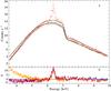 |
Fig. A.1 Top: observation of Vela X-1 (XMM-Newton ObsID 0111030101) made with the standard Timing Mode (red data points) and how the same observation would have looked like in the Modified Timing Mode (orange data points). Bottom: residuals of fitting these data with an absorbed power-law (red). Applying the same model and the standard Timing Mode matrix produces the residuals shown in orange, illustrating the softening. The residuals of a fit with the Modified Timing Mode response matrix (blue) agree with the Timing Mode residuals. |
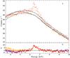 |
Fig. A.2 Same as Fig. A.1, but for an observation of Her X-1 (ObsID 0134120101) using the medium filter. |
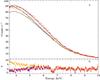 |
Fig. A.3 Same as Fig. A.1, but for an observation of Circinus X-1 (ObsID 0307420601) using the thin filter. |
The Modified Timing Mode response matrix used in this paper was obtained based on 82 thick filter observations (see Table A.1) and with a LET of 2.8 keV. Because the source was so bright, the inner three columns of the point spread function were discarded in the actual observations of Cyg X-1 used in our analysis. This effect was also taken into account in the construction of the response matrix.
To check how well the new response matrix can reproduce spectral features and to illustrate the effects of the increased LET we generated fake Modified Timing Mode observations of a set of bright sources using the tick, medium, and thin filters of the EPIC-pn camera (Fig. A.1–A.3). Figure A.1 shows the data points of the Timing Mode observation of the Galactic High Mass X-ray Binary Vela X-1 (XMM-Newton ObsID 0111030101; red data points). To illustrate the effects of the response matrices, we fit a simple absorbed power-law to these data (Fig. A.1, bottom). Removing all raw events below the LTE of 2.8 keV, and reconstructing again the event list results in the orange data points. Note that the loss of split partners below the LTE leads to a softening of the spectrum below about 5 keV. This is well illustrated in the residuals of the absorbed power-law fit if we apply the normal Timing Mode response matrix (orange data points). Using the Modified Timing Mode response matrix, on the other hand, yields residuals (and best fit values) which are identical to those of the Timing Mode observation. This illustrates that Pi,j was not affected significantly by statistical noise.
Similar calculations are shown in Figs. A.3 and A.2, which use the thin and medium filters, respectively. Even though no Modified Timing Mode observations exist which employ these filters, these measurements indicate that the calibration for these two filters is of similar quality as that for the thick filter.
XMM-Newton ObsIDs for medium filter observations used to produce the modified response matrix for the respective filter.
XMM-Newton ObsIDs for thin filter observations used to produce the modified response matrix for the respective filter.
Appendix B: Bright sources and the Charge Transfer Inefficiency (CTI)
Irrespective of the data mode bright source observations with XMM-Newton are affected by a further instrumental effect, namely the influence that the source photons have on the Charge Transfer Inefficiency of the detector. Like all X-ray astronomical CCDs the EPIC-pn suffers from contamination of the detector silicon (in the case of the EPIC-pn the contamination is due to titanium). This contamination causes traps in the silicon bulk which lead to a significant loss of the total generated signal charge when they are transferred to their closest read-out node. The effect is primarily dependent on the generated signal charge, and therefore the charge transfer efficiency (CTE) strongly correlates with the surface brightness on the CCD (Kendziorra et al. 1997). Calibration measurements for fainter observations allow us to model the CTE. Taking the measured source flux into account it is then possible to reconstruct the original event energy from its measured (CTE-affected) value. Using SAS v10 this correction works well for faint sources4, but for sources as bright as Cyg X-1 the CTE correction is highly nonlinear and cannot be modeled. Applying the standard CTE correction to such data inevitably leads to an overcorrection and finally wrong parameters describing the observed object. This forces us to apply a different approach using simultaneous or similar flux data from other X-ray missions.
As discussed in Sect. 2.4, in our analysis of Cyg X-1 we obtained the gain shift parameters from the simultaneous fit of the XMM-Newton data to the RXTE-PCA, -HEXTE, and INTEGRAL-ISGRI observations. This method is based on the assumption that the real energy of the photons, Ereal, is linearly related to the energy assigned by the SAS, Eobs,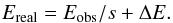 (B.1)Here s is the gain shift parameter and ΔE is an energy offset, which is expected to be 0 keV for CTE effects.
When performing a standard X-ray data analysis, individual photons are histogrammed into “spectra” with channel boundaries based on Eobs rather than Ereal, that is, the spectrum is distorted by the gain shift. In order to correct for the CTE we use a feature of ISIS that allows us to apply the energy bounds of the response matrix according to Eq. (1). A similar feature is also available in XSPEC (Arnaud 1996). Both, s and ΔE can be used in spectral fits, that is, by fitting an observation that is affected by an additional gain shift simultaneously with observations that are not affected by gain shift, it is in principle possible to recover s and ΔE. Here we demonstrate by a detailed comparison with other observations of the source that this approach yields indeed the correct value for the gain shift.
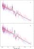 |
Fig. B.1 Gain shift in the EPIC-pn. a) Fit to the Chandra data. The model is composed of a broken power-law, an emission line at 6.4 keV and two absorption lines for Fe xxv and Fe xxvi. The two HEG datasets are presented in different colors. b) Applying a model taken from the fit to the EPIC-pn data and applied to Chandra data reveals the shift towards higher energies. Applying a gain-shift of ~2% to the EPIC-pn data corrects the fit and re-produces the good fit in a). The line widths were kept fixed for plotting purposes. |
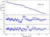 |
Fig. B.2 Gain shift correction of the EPIC-pn data. a) Fit to the EPIC-pn data of an absorbed power-law with narrow emission and absorption components from Chandra. b) Large residuals remain around 6.5 keV. c) Applying a gain-shift of ~2% to the EPIC-pn data improves the fit considerably. |
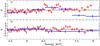 |
Fig. B.3 Test of the gain shift using RXTE data. a) Fit to the EPIC-pn (red) and PCA (blue) data with no gain-shift applied. There are large residuals, but also a slight energy shift between the instruments. b) Residuals after applying the gain-shift correction to EPIC-pn data. |
We use the XMM-Newton observation Obs2 for this example, as it is the most stable one in flux and since this observation is comparable in flux level to an archival Chandra observation of the source, namely Chandra ObsID 3814 (see Hanke et al. 2009, for a thorough analysis of the Chandra observation). Fitting the 5.5–8.0 keV band in the Chandra spectrum with an absorbed power-law reveals the presence of a narrow emission line at 6.4 keV and of two absorption lines from Fe xxv and Fe xxvi at  keV and
  keV (Fig. B.1a). Applying the best-fit Chandra spectrum to the EPIC-pn data leads to strong residuals around 6.5 keV (Fig. B.2b). The shape of the residuals is typical for a problem with the instrumental gain. Fixing the emission and absorption line energies to the values from Chandra, introducing a gain shift model and refitting improves the fit statistics to
  . The gain-shift slope is
  . Figure B.2 shows the significant improvement of the fit. The Fe emission line residuals have been removed and only small residuals remain at the location of the absorption lines. Since these occur in the wind and are strongly variable (Hanke et al. 2009; Miškovičová et al. 2016), this is not surprising.
As a cross check we work in the opposite direction and fit a continuum with absorption and emission lines to the EPIC-pn data without using the gain-shift. The emission line is found at E ~ 6.56 keV, the absorption lines at E ~ 6.73 keV and E ~ 7.0 keV. Applying this model to the Chandra data and only allowing the continuum to change does not result in a good fit. Figure B.1b clearly shows the misplacement, especially of the emission line (the absorption lines cannot be well constrained in the EPIC-pn spectra).
In order to further strengthen our results from line fitting, we use the absorption line parameters obtained from the Chandra data and fit the continuum to the joint XMM-Newton and RXTE data using a broken power law in the energy range 5.5–8.0 keV. Figure B.3 shows that a simple simultaneous fit leads to  , which is clearly an unacceptable value and the residuals are again indicative of a “best effort” of the fit to describe two incompatible spectral shapes (remember that these data were taken simultaneously). On the other hand, when a gain-shift of sgain ~ 1.024 is applied on the EPIC-pn data, the fit improves to
  (see Fig. B.3).
Best fit to the absorption lines seen in the Chandra data. τ describes the line depth and σ its width.
We conclude, therefore, that continuum fitting and the direct comparison of the location of distinct features (absorption/emission lines) gives consistent results and that a gain-shift of ~2% is needed in order to describe the EPIC-pn spectra. In Sect. 3 we therefore use the values from Table B.1 to describe features that the pn cannot resolve. For the different observations we also let the gain-shift slope sgainshift free since the above study indicates that for moderate energy shifts continuum fitting is sensitive enough to constrain the gain shift.
Appendix C: Full table values
Best fit parameters for a coronal model using a cutoff power-law and relativistic reflection with fixed emissivity index ϵ = 3 (Model 1).
Best fit parameters for a coronal model using a cutoff power-law and relativistic reflection with free emissivity index ϵ (Model 2).
Best fit parameters for a coronal model using a cutoff power-law and relativistic reflection where the emissivity follows a broken power-law (Model 3).
Best fit parameters for a lamp post model (Model 4).
All Tables
Best fit parameters for a coronal model using a cutoff power-law and relativistic reflection.
XMM-Newton ObsIDs for thick filter observations used to produce the modified response matrix for the respective filter.
XMM-Newton ObsIDs for medium filter observations used to produce the modified response matrix for the respective filter.
XMM-Newton ObsIDs for thin filter observations used to produce the modified response matrix for the respective filter.
Best fit to the absorption lines seen in the Chandra data. τ describes the line depth and σ its width.
Best fit parameters for a coronal model using a cutoff power-law and relativistic reflection with fixed emissivity index ϵ = 3 (Model 1).
Best fit parameters for a coronal model using a cutoff power-law and relativistic reflection with free emissivity index ϵ (Model 2).
Best fit parameters for a coronal model using a cutoff power-law and relativistic reflection where the emissivity follows a broken power-law (Model 3).
All Figures
|
Fig. 1 RXTE All Sky Monitor lightcurve of Cyg X-1 rebinned to a resolution of 1 d for the two year period surrounding the observations. The times of our four analyzed observations are marked with the vertical lines. Color coding corresponds to spectral state classification as defined by Grinberg et al. (2013): the blue color represents hard state, while the green color represents the intermediate state data. The inset is zoomed in on the four observations, with a resolution of one data point per spacecraft orbit. |
| In the text | |
|
Fig. 2 Broad residuals at the iron line region (around 6.4 keV) in XMM-Newton EPIC-pn observations are uncovered by excluding the 5.5–8.0 keV region and modeling the remaining data with a cutoff power-law. There are evident absorption features in the line spectra that are due to Fe xxv (6.65 keV) and Fe xxvi (6.96 keV) in the local medium. |
| In the text | |
|
Fig. 3 Background subtracted lightcurves for all four observations. Bottom panels: XMM-Newton and RXTE lightcurves, binned to a resolution of 96 s. Top panels: INTEGRAL-ISGRI lightcurves, binned to a resolution of 40 s. The black continuous line shows science window averaged count rates, i.e., averages over the ~30 min long individual INTEGRAL pointings. Data used in the analysis, i.e., data with roughly the same count rate level as that measured during the XMM-Newton observations, are shown in orange. Gray data points are from time intervals not used. The same flux variation is evident in all four instruments. Note that Obs4 is the shortest observation. See Table 1. |
| In the text | |
|
Fig. 4 Spectral modeling of the joint data. Top: unfolded XMM-Newton, RXTE and INTEGRAL data and best fit model components for the Corona geometry for Obs2. Blue line: continuum spectrum including the narrow iron Kα emission line and the black body. Purple line: relativistically smeared reflection component. Second panel: measured count rate spectra. The four lowest panels show the best fit residuals for observations Obs1–Obs4. EPIC-pn is blue, PCA is red, HEXTE is green and ISGRI is orange. |
| In the text | |
|
Fig. 5 Best fit XMM-Newton residuals for Corona geometry for observations Obs1–Obs4 for the fits of Fig. 4. No systematic variations are present. |
| In the text | |
|
Fig. 6 χ2 behavior of the spin a for the broken power law emissivity disk profile (Model 3). All four observations have their best minima at a ~ 0.9. Obs1 is drawn with solid, Obs2 with dashed, Obs3 with dotted and Obs4 dot-dash-dotted line. The zoom-in figure shows the area around the minima, produced with very fine binning. Similar behavior is produced for the single power-law profile. |
| In the text | |
|
Fig. 7 Parameter correlations for the coronal model with a cutoff power-law and relativistic reflection with ϵ fixed at ϵ = 3 and as a free parameter (Models 1 and 2 in Table 2). First row: holding the inclination fixed at i = 27° results in one best fit solution for the emissivity index ϵ and spin a. Second row: for i let free, one more solution emerges. We chose the physical one as the best fit (see Sect. 3.3.2). Third row: ϵ = 3 is chosen to describe the correlation between i and a. Fourth row: interplay between ϵ and i. Shown are the χ2 significance contours for two parameters of interest based on Δχ2 = 2.30, 4.61 and 9.21, i.e., 68%, 90% and 99% confidence levels, with respect to the best fit case. |
| In the text | |
|
Fig. 8 Parameter correlations for fits with a broken power-law emissivity (Model 3 in Table 2). High spin is required in all situations. First row: emissivity index ϵ and spin a. Second row: break radius rbreak versus the spin a. Third row: inclination i with respect to the spin a. Fourth row: change in emissivity profile index ϵ with varying break radius rbreak. Shown are the χ2 significance contours for two parameters of interest based on Δχ2 = 2.30, 4.61, and 9.21, i.e., 68%, 90%, and 99% confidence, with respect to the best fit case. |
| In the text | |
|
Fig. 9 Residuals for fits with the lamp post model for all four observations using XMM-Newton (blue), RXTE (PCA: red, HEXTE: green), and INTEGRAL (orange) data. |
| In the text | |
|
Fig. 10 Parameter correlations for the lamppost model (Model 4 in Table 3). Shown are the χ2 significance contours for the two parameters of interest. First row: jet base height h in units of GM/c2 versus the black hole spin a. Second row: inner disk inclination i expressed in degrees versus the spin a. The values clearly point towards a high spin value. Third row: inner disk inclination i versus the jet base height h. Shown are the χ2 significance contours for two parameters of interest based on Δχ2 = 2.30, 4.61, and 9.21, i.e., 68%, 90%, and 99% confidence, with respect to the best fit case. |
| In the text | |
|
Fig. A.1 Top: observation of Vela X-1 (XMM-Newton ObsID 0111030101) made with the standard Timing Mode (red data points) and how the same observation would have looked like in the Modified Timing Mode (orange data points). Bottom: residuals of fitting these data with an absorbed power-law (red). Applying the same model and the standard Timing Mode matrix produces the residuals shown in orange, illustrating the softening. The residuals of a fit with the Modified Timing Mode response matrix (blue) agree with the Timing Mode residuals. |
| In the text | |
|
Fig. A.2 Same as Fig. A.1, but for an observation of Her X-1 (ObsID 0134120101) using the medium filter. |
| In the text | |
|
Fig. A.3 Same as Fig. A.1, but for an observation of Circinus X-1 (ObsID 0307420601) using the thin filter. |
| In the text | |
|
Fig. B.1 Gain shift in the EPIC-pn. a) Fit to the Chandra data. The model is composed of a broken power-law, an emission line at 6.4 keV and two absorption lines for Fe xxv and Fe xxvi. The two HEG datasets are presented in different colors. b) Applying a model taken from the fit to the EPIC-pn data and applied to Chandra data reveals the shift towards higher energies. Applying a gain-shift of ~2% to the EPIC-pn data corrects the fit and re-produces the good fit in a). The line widths were kept fixed for plotting purposes. |
| In the text | |
|
Fig. B.2 Gain shift correction of the EPIC-pn data. a) Fit to the EPIC-pn data of an absorbed power-law with narrow emission and absorption components from Chandra. b) Large residuals remain around 6.5 keV. c) Applying a gain-shift of ~2% to the EPIC-pn data improves the fit considerably. |
| In the text | |
|
Fig. B.3 Test of the gain shift using RXTE data. a) Fit to the EPIC-pn (red) and PCA (blue) data with no gain-shift applied. There are large residuals, but also a slight energy shift between the instruments. b) Residuals after applying the gain-shift correction to EPIC-pn data. |
| In the text | |
Current usage metrics show cumulative count of Article Views (full-text article views including HTML views, PDF and ePub downloads, according to the available data) and Abstracts Views on Vision4Press platform.
Data correspond to usage on the plateform after 2015. The current usage metrics is available 48-96 hours after online publication and is updated daily on week days.
Initial download of the metrics may take a while.