| Issue |
A&A
Volume 588, April 2016
|
|
|---|---|---|
| Article Number | A134 | |
| Number of page(s) | 11 | |
| Section | Planets and planetary systems | |
| DOI | https://doi.org/10.1051/0004-6361/201527889 | |
| Published online | 30 March 2016 | |
Three-dimensional direct simulation Monte-Carlo modeling of the coma of comet 67P/Churyumov-Gerasimenko observed by the VIRTIS and ROSINA instruments on board Rosetta
1 Department of Climate and Space Sciences and Engineering, University of Michigan, Ann Arbor, MI 48109, USA
e-mail: fougere@umich.edu
2 Space Research and Planetary Sciences, University of Bern, 3012 Bern, Switzerland
3 LESIA, Observatoire de Paris, LESIA/CNRS, UPMC, Université Paris-Diderot, 92195 Meudon, France
4 INAF-IAPS, Istituto di Astrofisica e Planetologia Spaziali, via del fosso del Cavaliere 100, 00133 Rome, Italy
5 Belgian Institute for Space Aeronomy (BIRA-IASB), 1180 Brussels, Belgium
6 Institute of Computer and Netword Engineering, TU Braunschweig, 38106 Braunschweig, Germany
7 Lunar and Planetary Laboratory, University of Arizona, Tucson, AZ 85721, USA
8 Department of Space Science, Space Science and Engineering Division, Southwest Research Institute, San Antonio, TX 78238, USA
Received: 25 November 2015
Accepted: 1 February 2016
Context. Since its rendezvous with comet 67P/Churyumov-Gerasimenko (67P), the Rosetta spacecraft has provided invaluable information contributing to our understanding of the cometary environment. On board, the VIRTIS and ROSINA instruments can both measure gas parameters in the rarefied cometary atmosphere, the so-called coma, and provide complementary results with remote sensing and in situ measurement techniques, respectively. The data from both ROSINA and VIRTIS instruments suggest that the source regions of H2O and CO2 are not uniformly distributed over the surface of the nucleus even after accounting for the changing solar illumination of the irregularly shaped rotating nucleus. The source regions of H2O and CO2 are also relatively different from one another.
Aims. The use of a combination of a formal numerical data inversion method with a fully kinetic coma model is a way to correlate and interpret the information provided by these two instruments to fully understand the volatile environment and activity of comet 67P.
Methods. In this work, the nonuniformity of the outgassing activity at the surface of the nucleus is described by spherical harmonics and constrained by ROSINA-DFMS data. This activity distribution is coupled with the local illumination to describe the inner boundary conditions of a 3D direct simulation Monte-Carlo (DSMC) approach using the Adaptive Mesh Particle Simulator (AMPS) code applied to the H2O and CO2 coma of comet 67P.
Results. We obtain activity distribution of H2O and CO2 showing a dominant source of H2O in the Hapi region, while more CO2 is produced in the southern hemisphere. The resulting model outputs are analyzed and compared with VIRTIS-M/-H and ROSINA-DFMS measurements, showing much better agreement between model and data than a simpler model assuming a uniform surface activity. The evolution of the H2O and CO2 production rates with heliocentric distance are derived accurately from the coma model showing agreement between the observations from the different instruments and ground-based observations.
Conclusions. We derive the activity distributions for H2O and CO2 at the surface of the nucleus described in spherical harmonics, which we couple to the local solar illumination to constitute the boundary conditions of our coma model. The model presented reproduces the coma observations made by the ROSINA and VIRTIS instruments on board the Rosetta spacecraft showing our understanding of the physics of 67P’s coma. This model can be used for further data analyses, such as dust modeling, in a future work.
Key words: comets: general / comets: individual: 67P/Churyumov-Gerasimenko / methods: numerical / methods: data analysis / space vehicles: instruments
© ESO, 2016
1. Introduction
For the first time, a spacecraft is orbiting a comet for an extended period of time following the onset of the activity throughout the perihelion passage. The Rosetta mission provides unprecedented spatial and temporal information about the comet 67P/Churyumov-Gerasimenko (67P). Understanding the coma emergence from the surface of the nucleus is one main mission science goals of the Rosetta. The formation of the coma from the nucleus is still a relatively open question to this day. To correctly assess that question, a profound understanding of the activity of the nucleus is necessary. Indeed, as a result of the kinetic character of the constantly evolving coma, understanding the coma formation and the activity at the surface of the nucleus requires a comparison of theoretical models results and observational evidence.
The Rosetta Orbiter Spectrometer for Ion and Neutral Analysis (ROSINA) analyzes the cometary coma in situ. It is composed of three sensors, each optimized for part of the scientific objectives of the instrument: the Double Focusing Mass Spectrometer (DFMS), the Reflectron type Time-of-Flight mass spectrometer (RTOF), and the Comet Pressure Sensor (COPS). While COPS provides the total gas density at a given location in the coma, DFMS can provide the elemental and isotopic abundances of each gas species with a mass resolution of m/ Δm ≈ 3000 at the 1% peak level at a mass-to-charge ratio of 28 Da/e (Balsiger et al. 2007). Another Rosetta orbiter instrument, the Visual InfraRed Thermal Imaging Spectrometer (VIRTIS) provides remote sensing hyperspectral data from the near-ultraviolet (UV) through the near-infrared (IR) wavelengths. It is composed of two spectral channels. The channel VIRTIS-M takes hyperspectral images of the coma and nucleus of comet 67P, covering a wide range of wavelengths from the near UV (0.25 microns) to the near IR (5.0 microns). The channel VIRTIS-H is a very high spectral resolution point spectrometer in the near IR (Coradini et al. 2007).
The impressive images taken by the Deep Impact spacecraft in the context of the extended mission EPOXI during its fly-by of comet 103P/Hartley 2 revealed distinct outgassing patterns for H2O and CO2 (A’Hearn et al. 2011). This suggested that the sources of H2O and CO2 were not equally spread over the surface of the nucleus. Similarly, Hässig et al. (2015) observed heterogeneities in the coma of 67P with large fluctuations in composition from ROSINA data from August and September 2014. This was confirmed by the VIRTIS-H measurements of 67P from November 2014 to January 2015 (Bockelée-Morvan et al. 2015) and the VIRTIS-M mapping of very inner coma of 67P during mid-April 2015 (Migliorini et al. 2016). Indeed, the VIRTIS-M observations followed the evolution of the coma of comet 67P with an unprecedented spatial resolution of about 40 m/pixel, showing that H2O is mostly emanating from the neck connecting the two principal lobes, while CO2 emanates mostly from both the so-called head and southern latitude regions of the large lobe (Migliorini et al. 2016). Moreover, VIRTIS-M has observed the diurnal cycle of the water ice in the neck regions, occurring in the form of transient deposits formed in the upper layer of the surface by recondensation of water molecules sublimated from the subsurface ice (De Sanctis et al. 2015). The sublimation of these deposits during the morning time is directly correlated with the activity seen above these regions. Also, the analysis of the H O and H
 O (110−101) lines by the Microwave Instrument on the Rosetta Orbiter (MIRO) revealed a map of the H2O column density when the comet was at 3.4 AU of the Sun, showing higher values close to the “neck” region on the dayside, while low outgassing was present in the night side (Biver et al. 2015). The far-ultraviolet spectrograph Alice observed the H I and O I emissions resulting from electron dissociative excitation of H2O. These measurements suggested stronger emissions in the vicinity of the “neck” region as well (Feldman et al. 2015). Alice also showed that the C I emissions, which were attributed to electron dissociative excitation of CO2, varied with respect to those of H I and O I providing additional evidence of the heterogeneity of the coma (Feldman et al. 2015).
ROSINA and VIRTIS provide complementary information, which enable an extended probing of the coma of comet 67P. To accurately interpret the measurements from these two instruments, a coma model is necessary. Bieler et al. (2015) compared an analytical model based on illumination, a hydrodynamic simulation, and a direct simulation Monte-Carlo (DSMC) approach with ROSINA-COPS data. These authors showed that a model with the gas flux following the local illumination, assuming a uniform activity at the surface of the nucleus, could reproduce the COPS observations reasonably well. Also, Bockelée-Morvan et al. (2015) showed that such a model based solely on illumination was mostly able to explain the H2O measurements from VIRTIS-H. However, both studies found that a model assuming a uniform activity underestimated the H2O densities around the so-called neck area.
First, we present the H2O and CO2 DFMS data during the pre-perihelion period. Then, we give a description of the DSMC model, including the surface activity distribution retrieval using a spherical harmonics-based inversion method, which enables us to recover the nonuniform outgassing distribution from the nucleus of comet 67P. We show some direct outputs of the DSMC model for both species giving macroscopic parameters such as gas density and velocity in the cometary coma. Then, we compare results from the DSMC model with DFMS measurements and with a set of VIRTIS-M images of the H2O and CO2 coma taken at different illumination phases from Migliorini et al. (2016), and with VIRTIS-H column densities over a two month period from Bockelée-Morvan et al. (2015). Finally, the model is used to compute accurately the evolution of the H2O and CO2 production rates with heliocentric distance as observed by the various instruments. These are compared to ground-based observations of previous perihelion passages of comet 67P.
2. Data analysis and derivation
The results presented in this paper are based on data measured by two instruments on board the Rosetta spacecraft: ROSINA and VIRTIS. While a complete description and interpretation of the VIRTIS-M and -H data can be found in Migliorini et al. (2016) and Bockelée-Morvan et al. (2015), respectively, the ROSINA-DFMS data requires a more complete characterization because we present a substantial number of new measurements.
The DFMS is a neutral and ion mass spectrometer with a Nier-Johnson configuration (Balsiger et al. 2007; Johnson & Nier 1953). This spectrometer has a high dynamic range and a mass resolution of m/ Δm ≈ 3000 at the 1% peak level. In this study, we only focus on measurements of cometary neutrals. These neutrals enter the instrument’s ion source where they are ionized by a 45 eV electron impact beam. The resulting (positively charged) ions are then accelerated into the ion optics of the instrument. A position sensitive microchannel plate detector with two rows of 512 pixels along the dispersive axis of the instrument finally records the incoming ions. For our data analysis we take into account the irregular degradation of the 512 individual pixels over time. For this purpose dedicated measurement modes are performed every few weeks. In the case of overlapping peaks, the peak shapes are fitted with a Gaussian to evaluate the surface area providing the relative abundance of the different species. The (irregular) baseline of each spectrum is subtracted by fitting a 3rd degree polynomial through the sections of the spectrum not containing any peaks. We take into account fragmentation patterns and sensitivity values determined in the laboratory with the flight spare instrument. The signal contribution from the Rosetta spacecraft (Schlaäppi et al. 2010) has been characterized before arrival at 67P and is subtracted from the determined signal by DFMS. Figure 1 shows an example of DFMS data with the number of counts per spectrum of the H2O peak and the corresponding error. Finally, the sums of the relative abundances of the four major coma species (H2O, CO2, CO, and O2) are constrained such that added up they fit the total gas density measured by COPS. We focus solely on H2O and CO2 since the density evolution of most minor species is correlated to either one or the other of these two species (Luspay-Kuti et al. 2015).
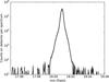 |
Fig. 1 Example of DFMS data showing the number of counts per spectrum of the H2O peak and the corresponding error. |
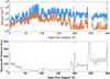 |
Fig. 2 Top panel: H2O (blue) and CO2 (orange) densities observed by the DFMS instrument from 4 August 2014 to 2 June 2015, bottom panel: spacecraft cometocentric distance in km. |
This approach is performed from 4 August 2014 up to 2 June 2015, a few days after equinox. Figure 2 shows the DFMS measured densities for the two species of interest for this study: H2O and CO2. The bottom panel shows the spacecraft distance from the comet. As expected, larger densities tend to be observed when the spacecraft is closer to the nucleus. Also, a general large-scale anti-correlation can be observed between H2O and CO2 in agreement with the RTOF measurements (Mall et al. 2016). A subset of this dataset was used by Hässig et al. (2015) to show the diurnal behaviors of H2O and CO2, which have two maxima per nucleus rotation. However, CO2 tends to show a maximum slightly shifted in time with respect to H2O, corresponding to the time when the Imhotep region (Thomas et al. 2015) is oriented toward the spacecraft (Hässig et al. 2015).
3. Description of the model
3.1. Generalities and boundary conditions
To describe the entire coma, including the regions where collisions cannot maintain the flow in a fluid regime, the use of a kinetic method is necessary. Hence, we apply a DSMC approach to solve the Boltzmann equation with the Adaptive Mesh Particle Simulator (AMPS) code (Tenishev et al. 2008, 2011; Fougere et al. 2013) to model the coma of comet 67P from the surface of the nucleus up to 400 km. This code was adapted and tested in 3D, enabling the use of irregular nucleus shapes (Fougere 2014). The coma model described in Fougere (2014) takes full advantage of the 3D character of the nucleus by using the local orientation of each triangular facet of the nucleus model with respect to the Sun to compute the local sublimating gas flux. We use a version of the triangulation of SHAP5.1 from the OSIRIS Science team (Preusker et al. 2015). The coordinate system used in the DSMC simulations follows the coordinate system from the nucleus shape model. The details regarding the collision cross-sections and physical processes (photodissociation, radiative cooling, etc.) included in the model are provided in Tenishev et al. (2008) and Fougere (2014).
The temperature at the inner boundary is deduced from the thermophysical model of Davidsson & Gutierrez (2004, 2005, 2006) showing variation with respect to the local solar illumination. The gas flux is computed for the kth nucleus triangular facet following the formula: 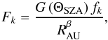 (1)where the function
  , simulating the variation of the flux with solar zenith angle similarly to the simulations presented in Bieler et al. (2015), is defined by
  (2)where anight is the flux ratio for a given location between conditions at local noon, i.e. when the triangle is directly oriented toward the Sun, and on the night side. As shown later, we find anight is 2% for H2O, which is a typical value according to the model of Davidsson & Gutierrez (2004, 2005, 2006), and 10% for CO2, which has a much lower sublimation temperature. ΘSZA is the local solar zenith angle, i.e. the angle between the normal of the triangle and the Sun direction. The self-shadowing of the nucleus is taken into account, and g = anight when a facet is in the shadow. The denominator in Eq. (1) simulates the general increase of gas production as the comet approaches the Sun. We assume that it follows a power-law with RAU, the comet heliocentric distance in units of AU, and we pick β = 4.2 for H2O (Hansen et al. 2015) and 2.0 for CO2. Finally, fk represents the heterogeneity of outgassing activity at the surface of the nucleus. Indeed, contrary to the assumption made in Bieler et al. (2015), it was observed extensively that the nucleus of comet 67P does not release gas in a uniform manner (Migliorini et al. 2016; Bockelée-Morvan et al. 2015; Biver et al. 2015; Feldman et al. 2015). The fk depends on the species type since the main regions of gas release have been observed to be different for H2O and CO2 (Hässig et al. 2015; Bockelée-Morvan et al. 2015; Migliorini et al. 2016). In our simulations, we describe the surface activity distributions of H2O and CO2 using a spherical harmonic expansion with 25 terms (i.e., of order 4) with constants determined by a least-squares method constrained by the ROSINA-DFMS data as described in the following section.
3.2. Description of the activity at the surface of the nucleus
Inhomogeneity in the gas release has been observed in several comets. Comet 103P/Hartley 2 was mostly releasing CO2 and icy grains from the subsolar lobe. Also, while most of the H2O from 103P/Hartley 2 was released in the form of large ice clumps of ~10 cm in size (Mumma et al. 2011), the H2O produced by the nucleus predominantly originated from the waist region as shown by the Medium Resolution Instrument images from the EPOXI mission (A’Hearn et al. 2011). A similar variation of source regions around the surface at comet 67P is suggested by the instruments observing the coma on board the Rosetta spacecraft (Hässig et al. 2015; Bockelée-Morvan et al. 2015; Migliorini et al. 2016; Biver et al. 2015; Feldman et al. 2015).
To reproduce the COPS data, Bieler et al. (2015) had to apply a latitude correction to the gas densities computed with a uniform surface activity model (see Figs. 5 and 6 from Bieler et al. 2015). This post-processing artificially increases the densities for positions in the coma with higher latitudes with respect to the rest of the coma. However, as a result of strong kinetic effects and nonradial motion of particles, the in situ gas density measured at a specific spacecraft latitude and longitude above the surface is not a direct indication of the source strength at the same latitude and longitude on the surface. Indeed, owing to fast gas expansion, small sources and outgassing features are lost within a few nucleus radii (Combi et al. 2012). Hence, a careful analysis is needed to clearly identify the gas sublimation pattern and identify the regions of the nucleus that release most of the gas observed in the coma.
To describe the activity at the surface of the nucleus, we decided to use spherical harmonics, ignoring the few regions that overlap because of the concavity of the nucleus. We use a least-squares method to obtain the best fit of the DFMS data with an analytical model to derive the undetermined coefficient for each spherical harmonic term. This model is an extension of the analytical model from Bieler et al. (2015), which proved to be a relatively good approximation of more complex and physically accurate models. In this study, the analytical model is used to describe the modeled gas density at the spacecraft location at the time of each DFMS data point from 4 August 2014 to 2 June 2015, a few days after equinox. These densities were then developed in spherical harmonics to create a M × N matrix (C), where M is the size of the DFMS/COPS data set (number of data points, ~17 000 for H2O and ~7000 for CO2) and N is the number of terms in the spherical harmonics expansion (here 25, i.e., up to order 4), defined as follows: 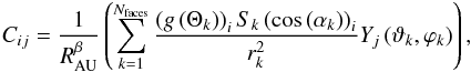 (3)where Nfaces is the total number of triangles meshing the nucleus, the function g is defined by similarly as in Bieler et al. (2015) by the following equation:
  (4)where the value anight is enforced when the triangle is in the shadows. The surface area of the kth triangle is Sk, rk and αk are the distance and angle between the spacecraft and the kth triangle, respectively. The parameter ϑk and ϕk are the colatitude and longitude of the center of the kth triangle from the nucleus model, respectively. Finally, the Yjs represent the different terms of the spherical harmonics.
Then, we need to solve a least-squares problem of the form  (5)where d is a vector of size M with elements containing the DFMS data, and x, the objective function, is a vector of size N representing the coefficients in front of the spherical harmonics, with the constraints that the activity described at a given triangle k by
  needs to be positive at all positions on the nucleus. This parameter fk is then be used in the inner boundary condition of the DSMC numerical model as described in Eq. (1).
This problem is solved with a standard constrained optimization iterative procedure detailed in Gould & Toint (2004). The best fit of the analytical model with the data, after applying the least-squares approach to derive the spherical harmonic coefficients, is illustrated in Fig. 3 with correlations of 0.84 and 0.83 for H2O and CO2, respectively. The analytical model is able to reproduce the large timescale anti-correlation between the two species. Indeed, it is clearly able to follow the evolution of the density measured by DFMS/COPS for both species during this period of ten months. The large-scale oscillation of the measured densities, with an amplitude of about 3 orders of magnitude over a few days for H2O and more than an order of magnitude for CO2, is relatively well reproduced by the model within a factor of 2 for the full period of ten months of data we considered. To better understand how well the model fits the data, we compute the root mean square coefficient of variation (rms-CV) defined as the root mean square deviation normalized by the mean measured value. We find that the rms-CV for H2O and CO2 are 1.14 and 1.08, respectively. Then, we can quantify improvement in the model ability to reproduce the DFMS data with respect to a model with a uniform activity. To do so, we apply the least-squares method with only the first constant term in the spherical harmonic expansion (order 0) to the H2O DFMS data, which returns the best fit with the assumption of a uniform activity. The corresponding rms-CV for the uniform activity case has a value of 2.03, which is about 80% higher than that computed with the 25-term spherical harmonic expansion discussed in this work.
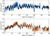 |
Fig. 3 Best fit of the analytical model (black) resulting from the optimization procedure with the DFMS data (blue for H2O and orange for CO2) from 4 August 2014 to 2 June 2015. |
Real spherical harmonics and the normalized corresponding coefficient found from the least-squares method for H2O and CO2.
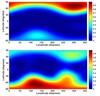 |
Fig. 4 Latitude/longitude mapping of the H2O (top) and CO2 (bottom) relative activity distribution at the surface of the nucleus described with a 25-term (order 4) spherical harmonic expansion. |
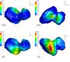 |
Fig. 5 H2O (top) and CO2 (bottom) relative activity distribution at the surface of the nucleus described with a 25-term (order 4) spherical harmonic expansion at the surface of the nucleus. The H2O peak emission is located in the Hapi region, while the CO2 emission is maximum south of the Imhotep region and above the Khonsu region following the nomenclature from Thomas et al. (2015). |
The optimization procedure leads to the activity distribution represented in Figs. 4 and 5, corresponding to the retrieved coefficients given by Table 1. This distribution follows the general observations with a dominant source of H2O released from the Hapi region of the nucleus following the nomenclature from Thomas et al. (2015), while more CO2 is produced in the southern hemisphere of the nucleus notably with the principal source south of the Imhotep region and above the Khonsu region. These results are consistent with the observations made by the different instruments on board Rosetta (Biver et al. 2015; Gulkis et al. 2015; Hässig et al. 2015; Bockelée-Morvan et al. 2015; Lee et al. 2015; Luspay-Kuti et al. 2015; Migliorini et al. 2016). Calculations by Keller et al. (2015) show that the total energy input close to the Hapi region is enhanced by reflected light and IR radiation from the walls of the local concavity, which could explain the H2O distribution of activity. Conversely, the identification of two areas in the Imhotep region, where exposed water ice is present in stable form at the surface, has been reported by Filacchione et al. (2016). However, the sparse illumination conditions, which occurred above these deposits before equinox, prevented the sublimation of the ice.
4. Simulation outputs
The DSMC simulations give access to a large number of macroscopic parameters, such as number density, velocity, kinetic temperature, and rotational temperature, and provide a full description of the coma of comet 67P.
The combination of the nonuniformity of the activity at the surface of the nucleus (previous section) and the local illumination imply that the flow is strongly asymmetric. Higher densities and speeds are observed where the surface is normal to the Sun direction and close to the identified main gas sources (Hapi region for H2O and south of the Imhotep region for CO2). Since the activity distributions are different for H2O and CO2, we notice very distinctive gas distributions in the resulting H2O and CO2 coma.
As an example to illustrate these points, Fig. 6 shows the local illumination at the surface of the nucleus on 23 December at 12:00 UT. The computation of the local solar angle is critical to derive the flux of gas that is released by each surface facet of the nucleus (see Eq. (1)). This is done taking into account self-shadowing from the nucleus itself due to the concave shape. Hence, the local illumination is computed as the cosine of the angle between the normal of each surface triangle and the direction of the Sun multiplied by a factor 0 if the triangle is in shadow and 1 if it is illuminated.
Figures 7 and 8 are DSMC model outputs of plane cuts of density and speed for H2O and CO2 on 23 December at 12:00 UT, respectively, out to 30 km from the nucleus. For that geometry, the H2O density ranges from about 1017 m-3 close to the Hapi region of the nucleus to a few times 1012 m-3 at 30 km from the nucleus. The CO2 density is between about 1015 m-3 close to the nucleus and appears more uniform than H2O since, at this time, the Sun was illuminating mostly the northern latitudes of the nucleus while the main source of CO2 was at a large solar zenith angle. At that time, the H2O speed reaches values of about 680 m s-1, which is consistent with MIRO observations (Gulkis et al. 2015).
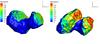 |
Fig. 6 Illumination on 23 December 2014 at 12:00 UT, i.e., the cosine of the angle between the Sun direction and each triangle normal multiplied by a factor 0 if the triangle is in shadows and 1 if the triangle is illuminated. |
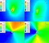 |
Fig. 7 DSMC outputs for H2O showing density distribution (top panels) in m-3 and speed (bottom panels) in m/s in the plane sections Y = 0 and Z = 0 for the case of 23 December 2014 at 12:00 UT. Each panel represents a square of 30 × 30 km. |
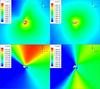 |
Fig. 8 DSMC outputs for CO2 showing density distribution (top panels) in m-3 and speed (bottom panels) in m/s in the plane sections Y = 0 and Z = 0 for the case of 23 December 2014 at 12:00 UT. Each panel represents a square of 30 × 30 km. |
5. Model comparison with instruments on board the Rosetta spacecraft
5.1. Model comparison with ROSINA-DFMS measurements
Since the boundary conditions of the model were determined by an analytical approach constrained using DFMS and COPS data, it is critical to verify that the outputs of the more rigorous DSMC model can reproduce these measurements. However, because of the nucleus rotation with a period of 12.4 h (Sierks et al. 2015), the parts of the nucleus that are directly illuminated by the Sun evolve. Also, as the comet approaches the Sun, the energy that the nucleus receives increases, and the Sun’s latitude slowly decreases. As a result of the large computational time required by the DSMC method, we cannot run a fully time-dependent simulation for an extended period. Instead, we extract the values from 48 steady-state simulations, where four full nucleus rotations are represented from 23 August 2014, 23 December 2014, 4 March 2015, and 6 May 2015 with a resolution of 1 h (12 simulations per nucleus rotation). To do so, from 4 August 2014 to 1 June 2015, we extract the solar latitude and longitude every hour. Then, we select the day from the simulation cases with the closest solar latitude with respect to the local latitude. Finally, we pick the case corresponding to the time with the closest solar longitude as the most representative.
By extracting the gas density of each species at the location of the spacecraft, we can directly compare the coma model with the DFMS/COPS observations (Fig. 9). The model clearly reproduces well the measured H2O and CO2 densities from August 2014 to June 2015. It also captures the seasonal variation of H2O and CO2, including their general anti-correlation. To take a closer look at the diurnal variation, Fig. 10 shows two weeks of DFMS data compared to the DSMC model during the second half of the month of October 2014. The model captures the maxima and minima for both H2O and CO2, notably the times when the Imhotep region is directed toward the spacecraft and the CO2 shows a maximum before H2O does as reported by Hässig et al. (2015). This validates the analytical approach that was used to derive the activity at the surface of the nucleus, and shows that the DSMC coma model is able to reproduce the ROSINA observations.
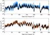 |
Fig. 9 Density extracted at the location of the spacecraft every hour from the DSMC outputs choosing the case from the 48 runs with the closest Sun/comet geometry. The top panel is for water with the DFMS/COPS in blue circles and the DSMC model in black. The bottom panel represents CO2 with DFMS/COPS data in orange and the DSMC model in black. |
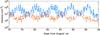 |
Fig. 10 Density extracted at the location of the spacecraft every hour from the DSMC outputs choosing the case from the 12 runs in August with the closest local time of the observation. Two weeks are represented showing the diurnal variation of H2O (blue) and CO2 (orange). The DFMS/COPS data is represented with circles and diamonds for H2O and CO2, respectively, while the model is illustrated with continuous lines. |
5.2. Model comparison with VIRTIS-M coma mappings
VIRTIS-M obtained maps of the very inner coma of comet 67P for emission bands of different species (Migliorini et al. 2016). A total of 74 observations were performed between 8 April and 14 April 2015 when the comet was at a heliocentric distance of about 1.9 AU. These observations clearly reveal that the main sources of H2O and CO2 are located at disparate locations at the surface of the nucleus (Migliorini et al. 2016), which is in agreement with the results shown in this paper. We focus on four of these observations covering different Sun/comet and spacecraft/comet geometries (Table 2). The duration of these observations covers time ranges from 18 to 24 min. For our DSMC simulations, we selected a typical time representative of the geometry at the times of observation (Table 2), neglecting the rotation of the comet during these 18−24 min of observation. The modeled column densities are then directly computed from the DSMC results by integrating the density along the line of sight from the spacecraft location to the boundary of the simulated domain.
Figure 11 compares the modeled H2O column density with four VIRTIS-M H2O images. In each VIRTIS-M image, the nucleus is masked to avoid high contrast among adjacent pixels that could generate undesirable scattering on the filter junctions. The mask is then enlarged by 7 pixels in all directions to take into account any uncertainty resulting from the nucleus shape model (Migliorini et al. 2016). This region is then also concealed in the model synthetic images. The agreement between the model and observations is evident with the part of the coma close to the Hapi region and directly illuminated by the Sun showing larger column densities up to about 8 × 10²⁰ m-2. Also, the model is able to capture smaller coma features not directly related to the most active regions of the nucleus, such as the coma feature seen close the southern latitudes of the nucleus on the image corresponding to observation I1_00387379010.
VIRTIS-M IR observations details (Migliorini et al. 2016) and corresponding times and gas production rates used in the DSMC runs.
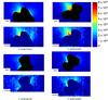 |
Fig. 11 H2O column density (in m-2) from the DSMC model (top image of each panel) compared with the corresponding VIRTIS-M observations (bottom image of each panel) from Migliorini et al. (2016) using a linear color scale from 0 to 8 × 10²⁰ m-2. |
Similarly, the juxtaposition between the CO2 synthetic images and the VIRTIS-M observations is represented in Fig. 12. The model reproduces rather well observations I1_00387379010, I1_00387481450, and to some extent I1_00387554894 with larger column densities coming from the southern latitudes of the nucleus and illuminated regions with column densities reaching a few 1019 m-2. However, some discrepancy appears between the model and observation I1_00387442903, where the CO2 distribution is somewhat different. Several effects may explain this disparity: we carried out the DFMS observations, which enabled us to retrieve the activity distribution at the surface of the nucleus, up to equinox when the Sun was mostly illuminating the northern latitudes. Hence, the retrieval for the southern latitudes may be less accurate. This might be further supported by the low resolution of the spherical harmonic description of the activity of the nucleus resulting in an uncertainty in the simulated coma and their inability to represent concavities. Moreoever, the fact that the nucleus rotated during the period of observation may be of importance for that particular geometry. Finally, the comet shows an intrinsic time variability of the outgassing not only due to the change of illumination. The model does not capture short-term inhomogeneities in the coma such as outbursts or jets appearing and disappearing over the time of hours.
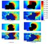 |
Fig. 12 CO2 column density (in m-2) from the DSMC model (top image of each panel) compared with the corresponding VIRTIS-M observations (bottom image of each panel) from Migliorini et al. (2016) using a linear color scale from 0 to 1 × 10¹⁹ m-2. |
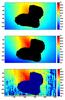 |
Fig. 13 log 10 of the H2O column density (in m-2) for the geometry of observation I1_00387442903 comparing a DSMC model with uniform surface activity (top panel), the DSMC model with a nonuniform surface activity defined with the spherical harmonics from this work (middle panel) compared with the corresponding VIRTIS-M observations (bottom panel) from Migliorini et al. (2016). |
In order to show the effect of the nonuniform surface activity on the resulting coma, we performed an additional DSMC simulation for the geometry of observation I1_00387442903 using the boundary conditions with a uniform surface activity from Bieler et al. (2015) and Bockelée-Morvan et al. (2015), where we scaled the total production rate to match the rate found in this work (5.0 × 1026 s-1 for H2O). Then, we proceeded to the same line-of-sight integration to simulate the synthetic image from this model with a uniform surface activity.
Figure 13 shows side-by-side the 10-based logarithm of the column densities to better show the coma structure and differences from the earlier model with uniform surface activity (Bieler et al. 2015), the model with the surface activity described with the use of spherical harmonics from this work, and the VIRTIS-M data. While the column density from uniform surface activity model is somewhat enhanced in the neck region because of the concavity of the surface, it underestimates the column density in this region by a factor of about 2 compared with the VIRTIS-M data and the new nonuniform model. Also, some high column densities appear at the bottom of the image derived from the uniform surface activity model on the night side of the nucleus that are not observed by VIRTIS-M, which was expected since the model presented in Bieler et al. (2015) was fitted to COPS data observing the total gas density without distinguishing species and includes contributions from highly volatile species like CO2 and CO. The model presented in this work agrees better with the VIRTIS-M data and gives better results regarding the distribution of both individual gas species in the coma of 67P.
5.3. Model comparison with VIRTIS-H data
Bockelée-Morvan et al. (2015) showed the first observations of H2O and CO2 in comet 67P by the VIRTIS-H instrument from 24 November to 24 January. These remote sensing observations were converted into column densities and the H2O data were compared to a DSMC coma model with a uniform nucleus surface, showing that the H2O column densities close to Hapi and Seth regions were underestimated by the model (Bockelée-Morvan et al. 2015). We present a model with a nonuniform surface leading to regions of the nucleus with different activity. Hence, we can reiterate the process that was applied in Bockelée-Morvan et al. (2015) with a more realistic nucleus outgassing. Also, we can make a direct comparison of our CO2 model with these observations.
Figure 14 shows a direct comparison of the modeled column densities from the DSMC model presented in this work in function of the observed VIRTIS-H column densities for H2O and CO2. The column densities from the model were computed by taking the average of values of the integrated density profiles along the line of sight at both the starting and ending times of observation corrected for the heliocentric distance using the power laws used in the model (β = 4.2 for H2O and 2.0 for CO2), which represent the lower and upper values of the error bars. We notice that the model can now correctly reproduce the larger H2O column densities observed by VIRTIS-H, which corresponds to the Seth and Hapi regions (Bockelée-Morvan et al. 2015), where we find the main source of H2O. This is an improvement with respect to the simpler model assuming a uniform surface activity that would consistently underestimate the column densities close to these regions and in agreement with the comparison made in the previous section with VIRTIS-M (Fig. 13).
Regarding CO2, the model follows the observations for most of the data points relatively well, showing a slope resulting from a linear regression close to 1. However, we observe that the model overestimates the column densities from observations I_00378954841 and I_00380112315, which both sustain the largest time-averaged solid angle from the Seth and Anuket regions (Bockelée-Morvan et al. 2015). This suggests that the model may somehow overestimate the CO2 released by these regions.
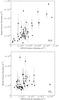 |
Fig. 14 Modeled column densities (in m-2) from the DSMC model we present in function of the observed VIRTIS-H column densities (in m-2) for H2O (top panel) and CO2 (bottom panel) from Bockelée-Morvan et al. (2015). The value is the average between the integration of the density profiles over the line of sight for both the starting and ending times of observation, which represent the upper and lower values by the error bars. |
6. Discussion
6.1. Evolution of the H2O and CO2 production rates
In previous sections, we showed that the model is able to reproduce the different observations made by the ROSINA and VIRTIS instruments on board the Rosetta spacecraft. Using the model results, we can get much more information regarding the coma’s properties and evolution.
As a result of strong asymmetries in the coma, deducing a gas production rate from a measurement is not straightforward. The use of a simple Haser model can give a rough estimate of the instantaneous production rate, but it is clear that it strongly overestimates the total production rate if the observation is made on the day side, while it underestimates the total outgassing when the spacecraft is above the night side. The spatial distribution of the sources and resulting coma gas distribution from this work can be used for a better estimate of the gas production rate. Hansen et al. (2015) derived an analytical formula to reproduce the average of a solely illumination-based coma model over a nucleus rotation period to derive a power law to follow the total gas production rate observed by COPS. With the model presented in this paper, we can derive H2O and CO2 production rates observed by both DFMS and VIRTIS. For each data point, we derive the expected density from the model for a given production rate using the case with the closest geometry among the 48 simulations. Then, to a first order approximation, the ratio between the observed density and the modeled density is equal to the ratio between the production rate deduced from the DFMS measurement and the rate used in the model run. We can operate similarly for VIRTIS-H using the ratio of the observed and modeled column densities. In the case of DFMS, we averaged over two-day periods of time (about four nucleus rotations).
These computations result in the H2O and CO2 production rates as a function of heliocentric distance (Fig. 15). Both VIRTIS and ROSINA production rates deduced from the model show good agreements with observations made during previous apparitions of comet 67P, both ground based (Schleicher 2006) and from the AKARI spacecraft (Ootsubo et al. 2012). The predictions made from light curve, ground-based measurements by Snodgrass et al. (2013) during its last perihelion passage agree well with the H2O production rate observed by DFMS and VIRTIS, while the CO2 predictions seem to be slightly overestimated. The model from Cowan & A’Hearn (1979), assuming that the spin axis tilt is perpendicular to the comet-Sun line with an active area of 2%, shows a weaker dependence with heliocentric distance. One could explain this by an increase of active area as the comet gets closer to the Sun, which could be due to erosion on the southern latitudes of the nucleus (Keller et al. 2015) enabling easier sublimation as these regions are illuminated.
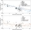 |
Fig. 15 Production rates resulting from DFMS/COPS, VIRTIS-H (Bockelée-Morvan et al. 2015), and VIRTIS-M (Migliorini et al. 2016) data deduced from the DSMC model for H2O (top panel) and CO2 (bottom panel). These values are compared to observations from Schleicher (2006) and Ootsubo et al. (2012), the predictions from Snodgrass et al. (2013), and the water sublimation model from Cowan & A’Hearn (1979). The continuous line represents the power law that was used in this work (β = 4.2 for H2O (Hansen et al. 2015) and 2.0 for CO2). |
6.2. Description of the CO2/H2O ratio in the coma of 67P
ROSINA measurements showed number density ratios of CO2/H2O ranging from 2.5% in the summer hemisphere to 80% in the winter hemisphere (Le Roy et al. 2015). VIRTIS provided observations of the CO2/H2O column density ratios in 67P’s coma with values between 2 and 60% (Bockelée-Morvan et al. 2015; Migliorini et al. 2016). Our model can give the evolution of these parameters with time and location in the coma. As an example, Fig. 16 shows the modeled column density ratios between CO2 and H2O in log 10 for the geometry of observation I1_00387379010. We observe that this ratio varies by an order of magnitude, depending which region of the coma is probed by the remote sensing instrument. The lower CO2/H2O column density ratios are found close to the Hapi region where the most active H2O region is located. Hence, due to the strong asymmetries in the coma, these measurements can only give some clues regarding the actual CO2/H2O ratio in terms of production rates without the use of a coma model.
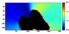 |
Fig. 16 log 10 distribution of the ratio between the modeled column densities of CO2 and H2O using the geometry of observation I1_00387379010. |
The difference of volatility between the two species implies that the mixing ratio of CO2 with respect to H2O tends to be higher at larger heliocentric distances. This is in agreement with the evolution of the production rates observed in Fig. 15, showing that the increase of the H2O production rate as the comet gets closer to the Sun is larger than that of CO2. Moreover, the rotation of the nucleus implies that different regions of the nucleus are illuminated at different times, which implies a diurnal variation of the CO2/H2O ratio due to their different activity distribution. Figure 17 shows the evolution of the ratio between the CO2 production rate (Q(CO2)) and the H2O production rate (Q(H2O)) for the cases used in the model. The Q(CO2)/Q(H2O) ratios are within 3 and 10% with variations of about 3% within one nucleus rotation period.
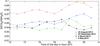 |
Fig. 17 Diurnal variation of the Q(CO2)/Q(H2O) ratio from the modeled DSMC cases. |
7. Conclusions
Using the least-squares fit of an analytical model to best fit the ROSINA DFMS data, we were able to construct the activity distribution at the surface of the nucleus for H2O and CO2, showing a nonuniform surface activity. H2O has a dominant source in the Hapi region, while CO2’s main source is located south of the Imhotep region. This activity distribution was coupled with our previous illumination driven model of surface activity to simulate the H2O and CO2 coma of comet 67P using a 3D DSMC model.
The densities measured by DFMS and the simulated densities from the DSMC model show good agreement both at the seasonal and at diurnal level, reproducing the general anti-correlation between H2O and CO2, and the accurate location of the two local maxima per nucleus rotation period.
A direct comparison to the impressive images taken by VIRTIS-M of the very inner coma of comet 67P (Migliorini et al. 2016) shows that the model captures the H2O coma structure even close to the nucleus. For CO2, most geometries show consistency between the model and the data. The remaining differences are probably because the data set that constrains the surface activity does not cover the post-equinox period and/or a rather low resolution of the activity distribution. In future work we will continue to apply our spherical harmonics fitting method to post-equinox and post-perihelion DFMS measurements, which should address some of these issues.
A similar comparison between our model and the VIRTIS-H data as in Bockelée-Morvan et al. (2015) was performed showing that the DSMC coma model presented in this work can reproduce H2O column densities. The previous model assuming uniform surface activity underestimated the column densities close to the “neck” region. Also, for the first time, we compared the CO2 VIRTIS-H data from Bockelée-Morvan et al. (2015) with our model, showing good agreement overall but with a potential overestimation close to the Seth and Anuket regions.
The model showed agreement with a large data set from different instruments, making a strong statement regarding our understanding of the coma of comet 67P. This model was able to reproduce the observations much better than a simpler model assuming a uniform surface activity. This model can be used as a tool for interpretation of other measurements made by the Rosetta spacecraft. The results presented in this paper can be extrapolated to minor species since their distributions are often correlated with either H2O or CO2 (Luspay-Kuti et al. 2015).
Using the coma model, we were able to convert the DFMS and VIRTIS measurements into gas production rates, which compare relatively well with previous observations of comet 67P and model predictions. Also, we show that the mixing ratio of CO2 with respect to H2O varies strongly within the coma and with nucleus rotational phase and heliocentric distance. Estimates of the ratio between CO2 and H2O in terms of total production rates were between 3% and 10%, and tended to decrease as the comet moved closer to the Sun due to the difference of volatility between the two species.
The modeling work of the gas coma of comet 67P presented here is critical for correctly computing the drag force exerted on the dust grains. While 3D DSMC dust coma simulations applied to comet 67P have already been performed (Fougere et al. 2014), we will run additional dust simulations building from this work and compare them with the relevant instrument data.
Acknowledgments
This work was supported by contracts JPL#1266313 and JPL#1266314 from the US Rosetta Project and NASA grant NNX09AB59G from the Planetary Atmospheres Program. Work at UoB was funded by the State of Bern, the Swiss National Science Foundation, and by the European Space Agency PRODEX Program. Work at Southwest Research institute was supported by subcontract #1496541 from the Jet Propulsion Laboratory. Work at BIRA-IASB was supported by the Belgian Science Policy Office via PRODEX/ROSINA PEA C4000107705 and an Additional Researchers Grant (Ministerial Decree of 2014-12-19), as well as by the Fonds de la Recherche Scientifique grant PDR T.1073.14 Comparative study of atmospheric erosion. ROSINA would not give such outstanding results without the work of the many engineers, technicians, and scientists involved in the mission, in the Rosetta spacecraft, and in the ROSINA instrument team over the last 20 years whose contributions are gratefully acknowledged. The authors would like to thank ASI, Italy; CNES, France; DLR, Germany; and NASA, USA for supporting this research. VIRTIS was built by a consortium formed by Italy, France, and Germany under the scientific responsibility of the Istituto di Astrofisica e Planetologia Spaziali of INAF, Italy, which also guides the scientific operations. The consortium also includes the Laboratoire dtudes spatiales et d’instrumentation en astrophysique of the Observatoire de Paris, France, and the Institut für Planetenforschung of DLR, Germany. The authors wish to thank the Rosetta Science Ground Segment and the Rosetta Mission Operations Centre for their continuous support. We thank the NASA Supercomputer Division at AMES for enabling us to perform the simulations presented in this paper on Pleiades supercomputers.
References
- A’Hearn, M. F., Belton, M. J. S., Delamer, W. A., et al. 2011, Science, 332, 1396 [NASA ADS] [CrossRef] [Google Scholar]
- Balsiger, H., Altwegg, K., Bochsler, P., et al. 2007, Space Sci. Rev., 128, 745 [NASA ADS] [CrossRef] [Google Scholar]
- Bieler, A., Altwegg, K., Balsiger, H., et al. 2015, A&A, 583, A7 [NASA ADS] [CrossRef] [EDP Sciences] [Google Scholar]
- Biver, N., Hofstadter, M., Gulkis, S., et al. 2015, A&A, 583, A3 [NASA ADS] [CrossRef] [EDP Sciences] [Google Scholar]
- Bockelée-Morvan, D., Debout, V., Erard, S., et al. 2015, A&A, 583, A6 [NASA ADS] [CrossRef] [EDP Sciences] [Google Scholar]
- Combi, M. R., Tenishev, V. M., Rubin, M., Fougere, N., & Gombosi, T. I. 2012, ApJ, 749, 29 [NASA ADS] [CrossRef] [Google Scholar]
- Coradini, A., Capaccioni, F., Drossart, P., et al. 2007, Space Sci. Rev., 128, 529 [NASA ADS] [CrossRef] [Google Scholar]
- Cowan, J. J., & A’Hearn, M. F. 1979, Moon and the Planets, 21, 155 [NASA ADS] [CrossRef] [Google Scholar]
- Davidsson, B. J. R., & Gutierrez, P. J. 2004, Icarus, 168, 392 [NASA ADS] [CrossRef] [Google Scholar]
- Davidsson, B. J. R., & Gutierrez, P. J. 2005, Icarus, 176, 453 [NASA ADS] [CrossRef] [Google Scholar]
- Davidsson, B. J. R., & Gutierrez, P. J. 2006, Icarus, 180, 224 [NASA ADS] [CrossRef] [Google Scholar]
- De Sanctis, C., Capaccioni, F., Ciarnello, M., et al. 2015, Nature, 525, 500 [NASA ADS] [CrossRef] [Google Scholar]
- Feldman, P., A’Hearn, M., Bertaux, J.-L., et al. 2015, A&A, 583, A8 [NASA ADS] [CrossRef] [EDP Sciences] [Google Scholar]
- Filacchione, G., De Sanctis, M. C., Capaccioni, F., et al. 2016, Nature, 529, 368 [NASA ADS] [CrossRef] [Google Scholar]
- Fougere, N. 2014, Ph.D. Thesis University of Michigan, 245 [Google Scholar]
- Fougere, N., Combi, M. R., Rubin, M., & Tenishev, V. 2013, Icarus, 225, 688 [NASA ADS] [CrossRef] [Google Scholar]
- Fougere, N., Tenishev, V., Bieler, A., et al. 2014, American Geophysical Union, Fall Meeting, abstract #P41C-3930 [Google Scholar]
- Gould, N., & Toint, P. L. 2004, Math. Program., 100, 95 [Google Scholar]
- Gulkis, S., Allen, M., Von Allmen, P., et al. 2015, Science, 347, 0709 [Google Scholar]
- Hansen, K. C., Fougere, N., Bieler, A., et al. 2015, American Geophysical Union, Fall Meeting, abstract #P31E-2104 [Google Scholar]
- Hässig, M., Altwegg, K., Balsiger, H., et al. 2015, Science, 347, 0276 [CrossRef] [Google Scholar]
- Johnson, E. G., & Nier, A. O. 1953, Phys. Rev., 91, 10 [NASA ADS] [CrossRef] [Google Scholar]
- Keller, H. U., Mottola, S., Skorov, Y., & Jorda, L. 2015, A&A, 579, L5 [NASA ADS] [CrossRef] [EDP Sciences] [Google Scholar]
- Le Roy, L., Altwegg, K., Balsiger, H., et al. 2015, A&A, 583, A1 [Google Scholar]
- Lee, S., Von Allmen, P., Allen, M., et al. 2015, A&A, 583, A5 [NASA ADS] [CrossRef] [EDP Sciences] [Google Scholar]
- Luspay-Kuti, A., Hässig, M., Fuselier, S. A., et al. 2015, A&A, 583, A4 [NASA ADS] [CrossRef] [EDP Sciences] [Google Scholar]
- Mall, U., Dabrowski, B., Korth, A., et al. 2016, ApJ, submitted [Google Scholar]
- Migliorini, A., Piccioni, G., Capaccioni, F., et al. 2016, A&A, in press, DOI: 10.1051/0004-6361/201527661 [Google Scholar]
- Mumma, M. J., Bonev, B. P., Villanueva, G. L., et al. 2011, ApJ, 734, L7 [NASA ADS] [CrossRef] [Google Scholar]
- Ootsubo, T., Kawakita, H., Hamada, S., et al. 2012, ApJ, 752, 12 [Google Scholar]
- Preusker, F., Scholten, F., Matz, K.-D., et al. 2015, A&A, 583, A33 [NASA ADS] [CrossRef] [EDP Sciences] [Google Scholar]
- Schlaäppi, B., Altwegg, K., Balsiger, H., et al. 2010, JGRE, 115, A12 [Google Scholar]
- Schleicher, D. G. 2006, Icarus, 181, 442 [CrossRef] [Google Scholar]
- Sierks, H., Barbieri, C., Lamy, P. L., et al. 2015, Science, 347, 1044 [NASA ADS] [CrossRef] [Google Scholar]
- Snodgrass, C., Tubiana, C., Bramich, D. M., et al. 2013, A&A, 557, A2 [Google Scholar]
- Tenishev, V., Combi, M. R., & Davidsson, B. 2008, ApJ, 685, 659 [NASA ADS] [CrossRef] [Google Scholar]
- Tenishev, V., Combi, M. R., & Rubin, M. 2011, ApJ, 732, 104 [Google Scholar]
- Thomas, N., Sierks, H., Barbieri, C., et al. 2015, Science, 347, 0440 [CrossRef] [Google Scholar]
All Tables
Real spherical harmonics and the normalized corresponding coefficient found from the least-squares method for H2O and CO2.
VIRTIS-M IR observations details (Migliorini et al. 2016) and corresponding times and gas production rates used in the DSMC runs.
All Figures
|
Fig. 1 Example of DFMS data showing the number of counts per spectrum of the H2O peak and the corresponding error. |
| In the text | |
|
Fig. 2 Top panel: H2O (blue) and CO2 (orange) densities observed by the DFMS instrument from 4 August 2014 to 2 June 2015, bottom panel: spacecraft cometocentric distance in km. |
| In the text | |
|
Fig. 3 Best fit of the analytical model (black) resulting from the optimization procedure with the DFMS data (blue for H2O and orange for CO2) from 4 August 2014 to 2 June 2015. |
| In the text | |
|
Fig. 4 Latitude/longitude mapping of the H2O (top) and CO2 (bottom) relative activity distribution at the surface of the nucleus described with a 25-term (order 4) spherical harmonic expansion. |
| In the text | |
|
Fig. 5 H2O (top) and CO2 (bottom) relative activity distribution at the surface of the nucleus described with a 25-term (order 4) spherical harmonic expansion at the surface of the nucleus. The H2O peak emission is located in the Hapi region, while the CO2 emission is maximum south of the Imhotep region and above the Khonsu region following the nomenclature from Thomas et al. (2015). |
| In the text | |
|
Fig. 6 Illumination on 23 December 2014 at 12:00 UT, i.e., the cosine of the angle between the Sun direction and each triangle normal multiplied by a factor 0 if the triangle is in shadows and 1 if the triangle is illuminated. |
| In the text | |
|
Fig. 7 DSMC outputs for H2O showing density distribution (top panels) in m-3 and speed (bottom panels) in m/s in the plane sections Y = 0 and Z = 0 for the case of 23 December 2014 at 12:00 UT. Each panel represents a square of 30 × 30 km. |
| In the text | |
|
Fig. 8 DSMC outputs for CO2 showing density distribution (top panels) in m-3 and speed (bottom panels) in m/s in the plane sections Y = 0 and Z = 0 for the case of 23 December 2014 at 12:00 UT. Each panel represents a square of 30 × 30 km. |
| In the text | |
|
Fig. 9 Density extracted at the location of the spacecraft every hour from the DSMC outputs choosing the case from the 48 runs with the closest Sun/comet geometry. The top panel is for water with the DFMS/COPS in blue circles and the DSMC model in black. The bottom panel represents CO2 with DFMS/COPS data in orange and the DSMC model in black. |
| In the text | |
|
Fig. 10 Density extracted at the location of the spacecraft every hour from the DSMC outputs choosing the case from the 12 runs in August with the closest local time of the observation. Two weeks are represented showing the diurnal variation of H2O (blue) and CO2 (orange). The DFMS/COPS data is represented with circles and diamonds for H2O and CO2, respectively, while the model is illustrated with continuous lines. |
| In the text | |
|
Fig. 11 H2O column density (in m-2) from the DSMC model (top image of each panel) compared with the corresponding VIRTIS-M observations (bottom image of each panel) from Migliorini et al. (2016) using a linear color scale from 0 to 8 × 10²⁰ m-2. |
| In the text | |
|
Fig. 12 CO2 column density (in m-2) from the DSMC model (top image of each panel) compared with the corresponding VIRTIS-M observations (bottom image of each panel) from Migliorini et al. (2016) using a linear color scale from 0 to 1 × 10¹⁹ m-2. |
| In the text | |
|
Fig. 13 log 10 of the H2O column density (in m-2) for the geometry of observation I1_00387442903 comparing a DSMC model with uniform surface activity (top panel), the DSMC model with a nonuniform surface activity defined with the spherical harmonics from this work (middle panel) compared with the corresponding VIRTIS-M observations (bottom panel) from Migliorini et al. (2016). |
| In the text | |
|
Fig. 14 Modeled column densities (in m-2) from the DSMC model we present in function of the observed VIRTIS-H column densities (in m-2) for H2O (top panel) and CO2 (bottom panel) from Bockelée-Morvan et al. (2015). The value is the average between the integration of the density profiles over the line of sight for both the starting and ending times of observation, which represent the upper and lower values by the error bars. |
| In the text | |
|
Fig. 15 Production rates resulting from DFMS/COPS, VIRTIS-H (Bockelée-Morvan et al. 2015), and VIRTIS-M (Migliorini et al. 2016) data deduced from the DSMC model for H2O (top panel) and CO2 (bottom panel). These values are compared to observations from Schleicher (2006) and Ootsubo et al. (2012), the predictions from Snodgrass et al. (2013), and the water sublimation model from Cowan & A’Hearn (1979). The continuous line represents the power law that was used in this work (β = 4.2 for H2O (Hansen et al. 2015) and 2.0 for CO2). |
| In the text | |
|
Fig. 16 log 10 distribution of the ratio between the modeled column densities of CO2 and H2O using the geometry of observation I1_00387379010. |
| In the text | |
|
Fig. 17 Diurnal variation of the Q(CO2)/Q(H2O) ratio from the modeled DSMC cases. |
| In the text | |
Current usage metrics show cumulative count of Article Views (full-text article views including HTML views, PDF and ePub downloads, according to the available data) and Abstracts Views on Vision4Press platform.
Data correspond to usage on the plateform after 2015. The current usage metrics is available 48-96 hours after online publication and is updated daily on week days.
Initial download of the metrics may take a while.