| Issue |
A&A
Volume 588, April 2016
|
|
|---|---|---|
| Article Number | A76 | |
| Number of page(s) | 14 | |
| Section | Galactic structure, stellar clusters and populations | |
| DOI | https://doi.org/10.1051/0004-6361/201527302 | |
| Published online | 22 March 2016 | |
Warp evidence in precessing galactic bar models
1 IEEC-UPC i Dept. de Matemàtiques, Universitat Politècnica de Catalunya, Diagonal 647 (ETSEIB), 08028 Barcelona, Spain
e-mail: This email address is being protected from spambots. You need JavaScript enabled to view it.
; This email address is being protected from spambots. You need JavaScript enabled to view it.
2 Dept. d’Astronomia i Meteorologia, Institut de Ciències del Cosmos, Universitat de Barcelona, IEEC, Martí i Franquès 1, 08028 Barcelona, Spain
e-mail: This email address is being protected from spambots. You need JavaScript enabled to view it.
3 GTM – Grup de recerca en Tecnologies Mèdia, La Salle, Universitat Ramon Llull, Quatre Camins 2, 08022 Barcelona, Spain
e-mail: This email address is being protected from spambots. You need JavaScript enabled to view it.
Received: 3 September 2015
Accepted: 15 January 2016
Abstract
Most galaxies have a warped shape when they are seen edge-on. The reason for this curious form is not completely known so far, so in this work we apply dynamical system tools to contribute to its explanation. Starting from a simple, but realistic model formed by a bar and a disc, we study the effect of a small misalignment between the angular momentum of the system and its angular velocity. To this end, a precession model was developed and considered, assuming that the bar behaves like a rigid body. After checking that the periodic orbits inside the bar continue to be the skeleton of the inner system even after inflicting a precession to the potential, we computed the invariant manifolds of the unstable periodic orbits departing from the equilibrium points at the ends of the bar to find evidence of their warped shapes. As is well known, the invariant manifolds associated with these periodic orbits drive the arms and rings of barred galaxies and constitute the skeleton of these building blocks. Looking at them from a side-on viewpoint, we find that these manifolds present warped shapes like those recognised in observations. Lastly, test particle simulations have been performed to determine how the stars are affected by the applied precession, this way confirming the theoretical results.
Key words: galaxies: kinematics and dynamics / galaxies: structure / galaxies: spiral
© ESO, 2016
1. Introduction
In this study we focus on the warps observed in some galaxies when seen edge-on. Thanks to the images of the Hubble Space Telescope and taking the probability of non-detection of warps into account when the line of nodes lies in the plane of the sky, it has been observed that nearly all galaxies are warped, confirming the suggestion made by Bosma (1981) for HI warps (Sánchez-Saavedra et al. 2003). Although there is abundant literature about this subject, the reason for these warps is not known yet. They have been observed in the distribution of stars (e.g. Sánchez-Saavedra et al. 1990) and in the study of neutral hydrogen (Bosma 1981), confirming that they are a very common phenomenon. In general, warps are commonly viewed as an integral sign as seen edge-on, manifesting themselves in the shape of the outer disc and bending away from the plane defined by the inner disc (like the galaxy shown in Fig. 1). This suggests some misalignment between the angular momenta of some material in warps and some material in the inner disc. In this direction, Debattista & Sellwood (1999) made simulations where the warp was formed when a misalignment between the angular momenta of the disc and the halo occurs.
Several assumptions have been made in the literature about the formation of warps. Briggs (1990) established some rules based on observational studies of external galaxies to determine the behaviour of galactic warps and claimed that warps appear from isophotal radius R26.5. After some time, Cox et al. (1996) studied the observations of the galaxy UGC 7170 concluding that due to the similarities between the stellar and gaseous warps, these could be produced by means of a gravitational origin. And more recently, Sellwood (2013) determined that since warps are really common, they should be either repeatedly regenerated or long-lived.
From a theoretical point of view, numerous approaches have been made to understand the mechanisms responsible for warp generation. One of these mechanisms, explained in Lynden-Bell (1965), established that warps could be produced by internal bending modes in the disc as a long-lived phenomenon, but this proposal held only for a disc with an unrealistic mass truncation (Hunter & Toomre 1969). In this context, Sparke & Casertano (1988) found warp modes inside rigid halos by means of discrete modes of bending. In Revaz & Pfenniger (2004), this discussion was revived and identified short-lived bending instabilities as a possible cause of the formation of warps, but obtaining warp angles of less than 5°. Nevertheless, Binney et al. (1998) argued that the inner halo would realign with the disc so the warp would dissipate.
Another possible explanation for the existence of warps is a tidal interaction between galaxies, a theory that has been studied to explain the Milky Way’s warp, mainly because of the proximity of the Large Magellanic Clouds (see e.g. Avner & King 1967; Hunter & Toomre 1969; Levine et al. 2006). Nevertheless, López-Corredoira et al. (2002) developed a method of calculating the amplitude of the galactic warp generated by a torque due to external forces. The method was applied to discard the tidal theory since it would lead to the formation of warps of very low amplitude. In fact, the authors proposed that warps are formed by the accretion of material over the disc (i.e. the accretion of angular momentum). Read et al. (2008) agree that the warp is an indicator of the merger activity and state that if the impact angle were larger than 20°, then the stellar disc could be warped.
As we can see, the explanation of the existence of warped galaxies represents a challenge. Our approach is based on the fact that warps are long-lived. By means of dynamical system tools, we take a simple, but widely used model composed of a bar and a disc to show that by introducing a natural misalignment between the angular momentum and the angular velocity, the model is consistent and is able to reproduce warped shapes. To check its consistency, we apply the fact that the periodic orbits are the backbone of galactic bars since these orbits are mainly stable, and therefore they mostly determine the structure of the bar (Contopoulos & Papayannopoulos 1980; Athanassoula et al. 1983; Contopoulos & Grosbøl 1989).
Then we study the set of orbits that depart from the Lyapunov orbits, proving that they acquire the warped shape with varying angles. The line of our study follows the analysis of the invariant objects that, in a similar dynamic way, cause the formation of rings and spiral arms in barred galaxies (Voglis & Stavropoulos 2005; Voglis et al. 2006; Patsis 2006; Romero-Gómez et al. 2006, 2007; Athanassoula et al. 2009). Again the purpose is to study the invariant manifolds associated with these objects. How these manifolds are affected by a precessing model and how this explains the appearance of galactic warps. Since invariant manifolds are determined by the potential of the galaxy, they exist for as long as this potential does not change significantly, thereby making them long-lived objects.
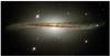 |
Fig. 1 Galaxy ESO 510-G13 photographed by the Hubble telescope. |
In Sect. 2 we justify the consistency of the misalignment between the angular momentum and angular velocity vectors and derive the equations of motion of the precessing model. We also describe the galactic potential considered and the characteristics of this potential in the precessing model. In Sect. 3 we describe the types of orbits inside the bar, observe how they are modified with the tilt angle, and check that they are the skeleton of the model. The formation of warps in our model is described in Sect. 4 where we study the invariant manifolds of the system that, as it is well known, provide the backbone of dynamics. In Sect. 5 we perform test-particle simulations of the model that, although they are collisionless simulations, serve to demonstrate that the orbits in the model behave as predicted. Finally, conclusions and expectations for future work are given in Sect. 6.
2. The precessing model
There are some theories that seek to explain the formation of warps through a misalignment between the angular momenta of the components of the models. Usually they assume that this is produced by the contribution of a third element, for instance, as an accretion of material due to the cosmic infall (see e.g. Ostriker & Binney 1989; Jiang & Binney 1999; López-Corredoira et al. 2002). It may also be aided by dynamical friction between the components (see e.g. Debattista & Sellwood 1999). Although this could be one of the reasons, the dynamics in the formation of the bar and other blocks of the galaxy could lead to a small misalignment between the angular velocity, ω, and the angular momentum, L, without any additional perturbation.
If we understand the galaxy and the formation of the bar as an accretion of material from a spinning mass distribution, the total angular momentum will be preserved during the process. However, for the angular velocity of its building blocks, even though the main component is in the direction of the angular momentum, a small component can appear in the orthogonal direction causing the misalignment. Probabilistically speaking, it is natural that it occurs in this way; moreover, it is reinforced by the existence of any other external perturbations or internal frictions. This is the result of having angular momentum, and angular velocity slightly misaligned in the motion of the bar should be a common phenomenon even when considering torque free motions of rigid bodies. In fact, the probability that L and ω are aligned is very low, if not zero. The result of this misalignment is a small precession of the bar.
Combes (1994) hypothesised about the relation between the precession of the angular momentum of a galactic disc and the formation of a warp as a vibration of the disc, but she did not pursue this idea any further. Although we reached the idea of studying the misalignment of the angular momentum and the angular velocity independently of Combes (1994), the work carried out in this paper may be considered, to some extent, to be a detailed study of the original question. Considering a galactic model formed by a bar and a disc, the main purpose of this paper is to study the effect of a small misalignment between the angular momentum of the system and its angular velocity.
The fundamentals of the motion of rigid bodies can be found in many books of classical mechanics (a classical reference e.g. Goldstein 1980). In what follows we summarize just a few main concepts that we need in order to introduce a precessing bar in a usual galactic model.
The main equation in rigid body dynamics relating angular momentum and angular velocity when they are expressed in a reference frame attached to the body is L = I·ω, where I is known as the inertia tensor. For the considered body frame, the tensor I is a symmetric constant matrix whose values only depend on the mass distribution. Since it is symmetric, this inertia tensor can be written in diagonal form, Ib = diag { I1,I2,I3 }, in an orthogonal basis. Its eigenvectors point to what are known as the principal axes of rotation, while the components I1, I2, and I3 are called principal moments of inertia. In the case of bodies with symmetric mass distributions, the principal axes are related to the symmetries. For instance, for a Ferrers bar (Ferrers 1877), independently of its degree of homogeneity, our first principal axis is aligned with the major axis of the bar in the x direction, while the remaining two ones are aligned with the major and minor axes of the ellipse obtained when cutting the Ferrers ellipsoid with the plane x = 0. Moreover, even though we will not be restricted to this case, for a constant density ellipsoid, the principal moments of inertia are given by  ,
,  , and
, and  , where Mb denotes the mass of the bar, and the parameters a (semi-major axis) and b, c (intermediate and semi-minor axes, respectively) define the shape of the bar.
Another main ingredient for modelling the motion of our precessing bar are the Euler equations. When assuming a torque-free motion, the angular velocity of the bar with respect to the static inertial axes, but expressed in the body frame (whose axes are aligned with the principal axes of the bar, see top panel of Fig. 2), ωb = (ω1,ω2,ω3) is a solution to Euler’s equations: 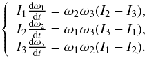 (1)We are going to study Eq. (1)in the case of an axially symmetric bar along the x axis, with parameters a>b = c. Since the major axis of the bar is along the x axis in body coordinates, we have I1 ≠ I2 = I3, and it immediately follows that ω1 and
  are constants of the motion. Then the angular velocity of the bar expressed in the body frame is
 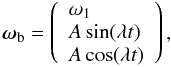 (2)where we have defined
 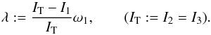 (3)We note that λ is the precession rate of ωb in a cone around the main axis of the bar.
 |
Fig. 2 Reference systems. Top: bar in the body reference frame, where the angular momentum Lb and the ybzb plane keep an angle ε. Bottom: bar in the inertial reference frame, where the angular momentum is aligned with the Z axis and the major axis of the bar keeps an angle ε with the XY plane. |
The angular momentum expressed in the body frame, Lb = Ib·ωb, has constant modulus  , and it describes a cone about the x axis. Let ε be the angle from Lb to the yz plane in the body reference (the angle between the generatrix of the cone, Lb, and the negative x semi-axis is
  , as is represented in the top panel of Fig. 2). We notice that in our study, ε will always be a small parameter. In terms of L and ε, the angular momentum of the bar in the body frame can be written as
  (4)Again we note that Lb has a small constant component, −Lsin(ε), in the x direction of the body frame and a big one of modulus Lcos(ε) describing a circle in the yz plane of the body frame. The angular velocity in the body frame is given by
  (5)It follows from Eqs. (3)and (5)that
  . Since the main axis, a, of the ellipsoid is much greater than the other axes, b and c, we find that I1<IT. Moreover, for low values of ε, sin(ε) ≈ ε, and therefore λ is also small. Finally let us note that when ε = 0, then λ = 0 and both, angular momentum and the angular velocity are aligned on the z axis.
Since the angular momentum, L, is preserved in an inertial reference frame, we take the inertial system so that the Z axis is aligned with L. The major axis of the bar has to keep an angle with respect to L, and then ε also measures the angle between the main axis of the bar and the XY plane of the inertial reference system. For this reason, from now on, it will be referred to as the tilt angle of the motion of the bar (see bottom panel of Fig. 2). In the inertial frame the major axis of the bar describes a cone about the Z axis, while L and ω are slightly misaligned since the bar is also rotating about its major axis. When ε = 0, the major axis of the bar rotates inside the XY plane, there is no rotation of the bar about its major axis, and L and ω are again aligned.
We define now a new non-inertial reference frame henceforth called the precessing reference system. In this reference frame, the x axis is aligned with the major axis of the bar, but the bar is not fixed as in the body frame but rotating around the x axis.
In the body reference system, the angular momentum and angular velocity vectors rotate around the main axis of the bar (x axis in the body frame) with angular speed λ. The precessing reference frame rotates with respect to the body frame about the x axis they share. This is, these frames are related by means of a time-dependent rotation of x axis and angular velocity λ, in such a way that ω and L are constant in the precessing reference system, with values of  (6)We are interested in the equations of motion of our galactic model in the precessing reference frame. To compute them, we need the angular velocity of the precessing frame with respect to the inertial one. This angular velocity, Ωp, is the sum of the angular velocity of the body, ωp, and the angular velocity of the body axes in the precessing frame. Therefore, and taking the value of λ into account, we obtain
 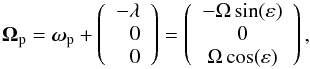 (7)where
  (see Chapter 2 of Sánchez-Martín 2015 for more details about the rotations).
Finally, as a complement, we briefly discuss the motion of the bar in the inertial frame. According to Poinsot’s theorem (see Arnold 1989), the bar, which is described by an ellipsoid, rolls without slipping on a fixed plane normal to the angular momentum L. If the ellipsoid has axial symmetry, as in our case, this motion is the superposition of a rotation of the ellipsoid along its symmetry axis with constant angular velocity, λ, and a precession with constant pattern speed Ω around the axis of the angular momentum. The tilt angle, ε, formed by the symmetry axis of the ellipsoid and the fixed plane remains constant.
It is also interesting to point out that when in our model we take ε = 0, the misalignment between the angular velocity and the angular momentum disappears, and we recover the classical model with pattern speed (0,0,Ω).
We have to emphasise here that this solution is valid for an axially symmetric rigid body, which in the case of the bar implies that the components b and c are equal, so that the moments of inertia I2 and I3 take the same value. If we want to treat the problem for the triaxial bar (b ≠ c), the equations of motion (10) that we present in the next section would not be autonomous, and this would introduce a complexity into the model that is not essential for our research. We see in the following sections, however, that the behaviour for a bar with b ≠ c is qualitatively the same and that the results for the axially symmetric and triaxial bar are essentially equivalent.
As for the location of the disc, we have to consider that we do not consider that the disc behaves as a rigid body, but it has to follow the main motion of the bar around the z-axis since the bar has been formed from the disc. We therefore include the disc in the equatorial xy plane of the model as a building block. Thus, the new model essentially provides a gravitational potential once the bar is formed, like many other traditional barred models (e.g. Contopoulos & Papayannopoulos 1980; Pfenniger 1984; Contopoulos & Grosbøl 1989) and generalises the fact that when the particles rearrange to form the bar, this is not just like a “parallel” arrangement with the main axes, but it may have small misalignments that make the bar precess inside the disc. Therefore, we can consider that the new model is a perturbation of order ε of the traditional bar plus axisymmetric component model. For clear reasons, this forces the value of ε to be low.
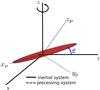 |
Fig. 3 Reference systems. The major axis of the bar is aligned with the precessing x axis, and the precessing z axis describes a cone about the inertial Z axis. Here (xp,yp,zp) denotes the precessing reference frame and (X,Y,Z) the inertial one. |
Of course, in a more realistic situation, the disc would be somewhat warped, but we have not included this possibility in the model because the small warped amplitude would not play an essential role in the gravitational potential that is already considered in the order of the thickness of the disc. On the contrary, a main point of the precessing model is that, owing to symmetries and by construction, the resulting system is autonomous, making it simpler.
2.1. Equations of motion associated with the precessing model
As is well known, the equation of motion of a particle in a rotating system is  (8)where r = (x,y,z) is the position vector of a star or a particle; φ = φd + φb is the potential of the system, which in our case is the sum of the potentials φd and φb of the disc and bar, respectively; and Ωp is the angular velocity given in Eq. (7). The second term on the right-hand side corresponds to Coriolis acceleration, and the last term to centrifugal acceleration.
To study the trajectories of stars under this potential, we consider the precessing reference frame as shown in Fig. 3. The equations of motion for our precessing reference system, hereafter referred to as the precessing model, are obtained by substituting the pattern speed (7)in Eq. (8), 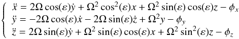 (9)where ε is the tilt angle, Ω the modulus of the pattern speed, and φ the potential (φ = φb + φd).
By setting (x1,x2,x3,x4,x5,x6) = (x,y,z,ẋ,ẏ,ż), the system (9) can be written as a system of first-order differential equations, 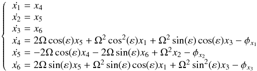 (10)where we recover the classical model when ε = 0. It is also worth mentioning that the precessing model has a Jacobi first integral given by
 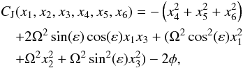 (11)and the effective potential is defined by
 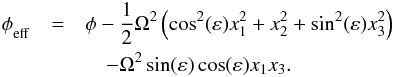 (12)
(12)
The Jacobi integral is related to the Hamiltonian character of the system. In fact, and as in the non-precessing case, CJ = −2H, where the Hamiltonian in the precessing reference system is 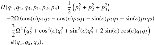 (13)where (pi, qi) is the momenta and positions, respectively, in Hamiltonian coordinates defined as
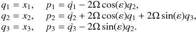
2.2. The galactic bar potential
As mentioned above, our galactic model consists of the superposition of an axisymmetric disc plus an ellipsoidal bar. In this paper and in Romero-Gómez et al. (2006), we essentially consider the same potential as in Pfenniger (1984). The disc component is modelled by a Miyamoto-Nagai potential (Miyamoto & Nagai 1975),  (14)where R2 = x2 + y2, and z denotes the distance in the out-of-plane component. The parameter G is the gravitational constant, and Md is the mass of the disc. The parameters A and B characterise the shape of the disc. Parameter A measures the radial scale length of the disc, while B is a measure of the disc thickness in the z direction. Since galactic discs are larger in the radial direction than in the vertical one, A is greater than B.
The barlike part is modelled by a Ferrers ellipsoid (Ferrers 1877) with a density function,  (15)where m2 = x2/a2 + y2/b2 + z2/c2. The parameters a (semi-major axis) and b, c (intermediate and semi-minor axes) determine the shape of the bar, parameter nh determines the homogeneity degree for the mass distribution,
  is the central density if nh = 2, and Mb the mass of the bar. This model concentrates matter in the central region and decreases smoothly towards zero at a finite distance.
The density of the bar potential is related with its potential, φb, by means of the Poisson equation (∇2φ = 4πGρ):  (16)where G is the gravitational constant, Δ(u) = (a2 + u)(b2 + u)(c2 + u), and
  the unique positive solution of
  if m ≥ 1 (that is, if the particle lies outside the bar), and zero otherwise.
The length unit used throughout this work is the kpc, the time unit is ut = 2 × 10⁶ yr, and the gravitational constant G = 6.674 × 10⁻¹¹ m3 kg-1 s-2. In this paper we take values A = 3, B = 1 for the disc, and for the bar we are going to consider two different Ferrers bars, one symmetric and another one with the values taken by Pfenniger (1984). For both bars, the homogeneity index is set to nh = 2 and the semi-major axis of the bar to a = 6. Whereas the first bar has revolution symmetry with semi-minor axes b = c = 0.95, the second bar only has axial symmetry with b = 1.5 ≠ c = 0.6. Some other parameters are considered to vary within a range: GMd ∈ [0.6,0.9], GMb ∈ [0.1,0.4] (but keeping in mind that G(Md + Mb) = 1). Finally we also consider the pattern speed Ω ∈ [0.05,0.06] [ut]-1 (~[24.46,29.36] km s-1/kpc) and the tilt angle ε ∈ [0,0.2] rad = [0,11.46] °.
A useful property for studying the matter distribution in galactic models is the rotation curve or circular speed Vrot(r), defined as the speed of a particle of negligible mass in a circular orbit at radius r. For a potential φ, we define Vrot as  (17)Although we have not imposed a halo potential, the rotation curve of the total potential, composed by the Ferrers bar and the Miyamoto-Nagai disc, is rather flat in the outer parts (see Fig. 4).
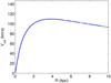 |
Fig. 4 Rotation curve of the potential φ = φb + φd. |
2.3. Characteristics of the precessing model
We define zero velocity surfaces of the precessing model as the manifold (x1,x2,x3) ∈ R3 defined by Eq. (11) with x4 = x5 = x6 = 0 for a given value of the Jacobi integral CJ. Their cut with the z = 0 plane defines zero velocity curves and the regions where φeff>CJ are forbidden regions for a star of the given energy (see Fig. 5).
As in the case ε = 0, our precessing model in rotating coordinates has five Lagrangian equilibrium points (Li, i = 1...5), solutions of ∇φeff = 0. These are represented in Figs. 5 and 6. As for the properties of these libration points when ε = 0, L1, and L2 lie on the x-axis and are symmetric with respect to the origin. Here, L3 lies on the origin of coordinates, L4 and L5 lie on the y-axis, and they are also symmetric with respect to the origin (see the upper panel of Fig. 5). The two equilibrium points, L1 and L2, are unstable, while L3 is linearly stable, and it is surrounded by the x1 family of periodic orbits, which is responsible for maintaining the bar structure, while the stable points L4 and L5 when ε = 0 have been thoroughly examined and are surrounded by families of periodic banana orbits (Athanassoula et al. 1983; Contopoulos 1981; Skokos et al. 2002a).
In our precessing model, we notice that whereas L3, L4, L5 maintain their coordinates fixed independently of ε, L1 and L2 vary as ε changes. Of relevant importance is the out-of-plane z-component for L1 and L2 (see bottom panel of Fig. 5). In Fig. 6 we detail the evolution of the coordinates of the equilibrium point L1 when the parameter ε varies from ε = 0 to ε = 0.2.
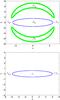 |
Fig. 5 Equilibrium points of the precessing model with GMb = 0.1. Top: xy plane with zero velocity curves for a Jacobi constant CJ = −0.1876. Bottom: xz plane, “+” for ε = 0, “×” for ε = 0.1, “•” for ε = 0.2, while the “∗” shows the position of the central L3 point. The blue curve in both panels outlines the triaxial Ferrers bar. |
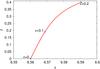 |
Fig. 6 Variation of the xz coordinates of L1 as ε varies within the range ε ∈ [0,0.2] for the precessing model with GMb = 0.1. The marked dots show the L1 coordinates for three specific values of ε: ε = 0 (bottom part of the plot), ε = 0.1 (middle), and ε = 0.2 (top). |
3. The structure of periodic orbits inside the bar
To understand the formation, evolution and properties of any given structure, it is essential to first understand its building blocks. In the case of galactic dynamics and, particularly, for barred galaxies, it has been clearly demonstrated that some building blocks are periodic orbits elongated along the bar. The study of these building blocks has provided answers to a number of crucial questions, such as why bars are bisymmetric, why they rotate as rigid bodies, and why they cannot extend beyond corotation (see Contopoulos 1981; Athanassoula et al. 1983; Pfenniger 1984; Skokos et al. 2002a, among others).
In this section we start from the infinitesimal periodic orbits about the central equilibrium point L3 and, considering either the period or the energy, continue the families of periodic orbits inside the bar at the same time as we study their stability properties. We therefore obtain evidence that the stable orbits we find give structure to the bar, since stars or particles can be trapped in their neighbourhood. All the integrations in this work were carried out numerically using a Runge-Kutta-Fehlberg method of orders 7–8. This method not only assures the conservation of the Jacobi constant, but it also provides the required accuracy for the detection of periodic orbits in the dynamical system.
With this aim, we first analyse the stability of the equilibrium point L3 in the precessing model. Let us consider the differential matrix around any Lagrangian point of the system (10): 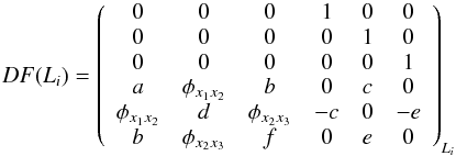 (18)where
 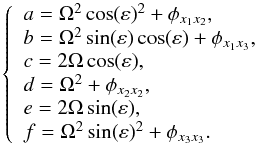 (19)For the particular case of L3, the eigenvalues of (18) are of the form { λi, −λi, μi, −μi, ωi, −ωi } (λ, μ, ω∈ R+) for any selected value of ε. Since the purely imaginary eigenvalues are associated with infinitesimal librations, the linearised flow around L3 in the rotating frame of coordinates is characterised by a superposition of three oscillations. This means that the L3 Lagrangian point is a linearly stable elliptic point, and in dynamical systems, this behaviour is usually denoted by the form centre×centre×centre. In our case it has two central components inside the xy plane and another one in the z direction.
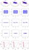 |
Fig. 7 Family of periodic orbits of the precessing model with b ≠ c and GMb = 0.1 (first row: 3D view; second, third, and fourth rows: (x,y), (x,z), and (y,z) projections, respectively) and stability indexes (bottom row) for ε = 0,0.1,0.2 (left, middle and right columns, respectively). In the first four rows, the red dashed lines outline the position of the triaxial Ferrers bar, while the blue lines are periodic orbits of the precessing model. In the bottom row: dark magenta (brown) lines indicate the b1 (b2) stability index. |
Next, following the work of Pfenniger (1984), which is a particular case of the precessing model with ε = 0, and following Broucke (1969), Hadjidemetriou (1975), we define the stability indexes of the periodic orbits, b1, b2:  (20)With these definitions, a periodic orbit is stable only when b1 and b2 are real and | b1 | , | b2 | ≦ 2, otherwise it is unstable. If | b1 | or | b2 | = 2, the Jacobian matrix of the continuation process is degenerate, and bifurcations of the family are allowed. If bi = + 2, the bifurcation occurs through period doubling, while if bi = −2, the bifurcation keeps the same period.
In the left-hand panel of Fig. 7, we show the results obtained for GMb = 0.1,Ω = 0.05, and ε = 0, which appears in Fig. 4 of Pfenniger (1984) for reference. In this figure, red dashed lines show the contour of the bar with semi-axis a = 6,b = 1.5,c = 0.6 in each plane, whereas blue lines indicate the x1 family of periodic orbits of the model and its bifurcations.
In a two-dimensional model, the x1 family of planar periodic orbits about L3 is mainly stable and has been regarded as responsible for the skeleton of the bar’s structure. But, in three-dimensional models, the backbone of the bars is the x1 family, together with its 3D bifurcating families (Skokos et al. 2002a,b). A continuation process in ε is then used to obtain parallel results for the tilt angle ε ≠ 0.
The results obtained in continuing the x1 family and its bifurcations for ε = 0.1 and ε = 0.2 are shown in the middle and right-hand panels of Fig. 7. Owing to the nature of the tilting, the most significant change is in the z component. The xy projections essentially remain the same, and the families of periodic orbits continue giving structure to the bar, as displayed in Fig. 8 where the families for ε = 0 and ε = 0.2 are compared. In this figure, red (green) lines show the position of the bar for ε = 0 (ε = 0.2). Blue (purple) lines indicate the periodic orbits of the model for ε = 0 (ε = 0.2).
In the last row of Fig. 7, we compare the stability indexes. For a given value of ε, b1 and b2 cross the limits (±2) an equal number of times and approximately at the same value of the Jacobi constant, CJ. All these facts again reinforce the evidence that the families of periodic orbits about L3 for any ε are qualitatively the same.
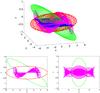 |
Fig. 8 Family of periodic orbits of the precessing model with b ≠ c for ε = 0 (blue) and ε = 0.2 (purple) and GMb = 0.1. From top to bottom: 3D view, xz-plane (left), yz-plane (right). Red (green) lines show the position of the bar for ε = 0 (ε = 0.2). Blue (purple) lines indicate the periodic orbits of the model for ε = 0 (ε = 0.2). |
At this moment, we can prove that although the equations given in Sect. 2 are for the case in which b = c in the bar, the results given in this section for the axially symmetric model remain the same. To prove this statement, we show in Fig. 9 how the periodic orbits and the stability indexes remain unchanged for b = c (following the same colour convention as in Fig. 7). To compare the symmetric case (b = c) with the non-symmetric one (model given in Pfenniger 1984 with b = 1.5 ≠ c = 0.6), we impose in both models equal bar mass (GMb = 0.1), equal homogeneity (nh = 2), and therefore equal particle distribution. Thus, we take a symmetric bar where the parameters  and
and  are the geometric mean of the previous parameters, i.e.
  . This results, somehow, in a gravitational field that is the average along time of the previous one.
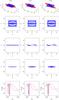 |
Fig. 9 Family of periodic orbits of the precessing model with b = c = 0.95 and GMb = 0.1 (first row: 3D view; second, third, and fourth rows: (x,y), (x,z), and (y,z) projections, respectively) and stability indexes (bottom row) for ε = 0,0.1,0.2 (left, middle, and right columns, respectively). In the first four rows, the red dashed lines outline the position of the triaxial Ferrers bar, while the blue lines are periodic orbits of the precessing model. In the bottom row: dark magenta (brown) lines indicate the b1 (b2) stability index. |
Comparing Figs. 7 and 9, we can confirm that the family of periodic orbits around the central equilibrium point L3 essentially remains the same, independently of whether we use a symmetric bar. Moreover, observing the stability indexes for both models (bottom panels), periodic orbits are in a comparable range of values of the Jacobi constant, where the cuts of the indexes within the limits | ± 2 | are qualitatively equal.
Therefore, we can conclude this comparison by saying that in both models, namely the one with revolution symmetry and the one that is axially symmetric, the periodic orbits are responsible for maintaining the structure of the bar and giving consistency to the model. In this way, we could use any of both models, but since a bar with parameters b ≠ c is more commonly used and we want to compare with the model given in Pfenniger (1984) to prove that our model is consistent although we apply a tilt, we prefer to show the rest of results for b ≠ c.
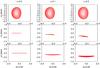 |
Fig. 10 Lyapunov family of periodic orbits around L2 for the model with GMb = 0.1 and for a range of values of the Jacobi constant in (CJ,L2,CJ,L2 + 2 × 10⁻³), where CJ,L2(ε = 0) = −0.1879, CJ,L2(ε = 0.1) = −0.1876 and CJ,L2(ε = 0.2) = −0.1865. The tilt angle ε ∈ [0,0.2]. Note the varying scale of the vertical axis. |
4. The invariant manifolds in the precessing model
Once we have analysed the behaviour of periodic orbits inside the bar, we continue the study by considering trajectories outside the bar that are responsible for the main visible building blocks in the barred galaxies, such as spirals and rings, i.e. the normally hyperbolic invariant manifolds associated to the libration point orbits about L1 and L2. The set of these orbits is responsible for the transport of matter between the neighbourhood of the bar and the exterior part of the galaxy. The stars trapped in these manifolds make their structure visible in the form of rings and arms. The rings and spirals obtained are response rings and spirals from the bar potential, and they are not imposed in the galactic potential, which means that they are not self-gravitating.
We study now the stability character of the libration points L1 and L2. The eigenvalues of the differential matrix (18) around L1 and L2 are of the form { λ, −λ, μi, −μi, ωi, −ωi } (λ, μ, ω∈ R+) for any value of ε. This means that the two real eigenvalues are related to a hyperbolic behaviour like a saddle, whereas the purely imaginary are associated to libration motions. This implies that the linearised flow around L1 and L2 in the rotating frame of coordinates is characterised by a superposition of a saddle and two harmonic oscillations, and in dynamical systems, this is usually described as a saddle×centre×centre behaviour. Then L1 and L2 are unstable and are called hyperbolic points. The dynamics around the unstable equilibrium points in our context are described in detail in Romero-Gómez et al. (2006) and Canalias & Masdemont (2006). Here just a brief summary follows.
As is well known, around each unstable equilibrium point, L1 and L2, there must exist a family of periodic orbits associated with the eigenvalues of the elliptical part. They are the planar and vertical families of Lyapunov periodic orbits. These orbits are unstable in the vicinity of the equilibrium point. The vertical family of Lyapunov orbits has been computed in galactic potentials (e.g. Ollé & Pfenniger 1998; Romero-Gómez et al. 2009) and its structure is different from the planar family shown in Fig. 10. The vertical family extends to both sides of the galactic plane, while the planar family in the precessing model when the parameter ε ≠ 0 remains on one side of the galactic plane without crossing it. Furthermore, in Romero-Gómez et al. (2009), it is shown that the family relevant to the transfer of matter within the galaxy is the planar family. Therefore, in the following we restrict our study to the planar family. In the second and third rows of Fig. 10, we show the xz and yz projections of Lyapunov orbits. It can be clearly seen from the yz projection that the orbit acquires some out-of-plane curvature when the parameter ε increases. Moreover, the z components of the orbit decrease with ε. (Keeping in mind that we are showing the Lyapunov orbits about L2, the opposite happens for the ones about L1.) This means that the libration point and the orbit are not strictly contained in the plane z = 0 when ε ≠ 0,and the periodic orbits are moreover not strictly planar.
For a given Jacobi constant, two sets of asymptotic orbits emanate from the periodic orbit. They are known as the stable and the unstable invariant manifold, and each set has two branches (see Fig. 11).
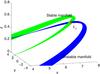 |
Fig. 11 Stable and unstable invariant manifold associated to the periodic orbit around L1 with ε = 0.2 and GMb = 0.3. |
We denote by  the stable invariant manifold associated to the periodic orbit γi around the equilibrium point Li, i = 1,2. This stable invariant manifold is the set of orbits that tend to the periodic orbit asymptotically forward in time. On the other hand, we denote by
  the unstable invariant manifold associated to the periodic orbit γi around the equilibrium point Li, i = 1,2. The unstable invariant manifold is the set of orbits that departs asymptotically from the periodic orbit (i.e. orbits that tend to Lyapunov orbits backwards in time). Since the invariant manifolds extend well beyond the neighbourhood of the equilibrium points, they are responsible for the large-scale structures and the transport of matter.
In Figs. 12 (Ω = 0.05) and 13 (Ω = 0.06), we show the (x,y) projection of the invariant manifolds of Lyapunov orbits around the equilibrium points, L1 and L2, varying with the tilt angle, the angular velocity or the bar mass, for the precessing model. In both figures we have chosen the values GMb = 0.1 and GMd = 0.9 for the first row, GMb = 0.2 and GMd = 0.8 for the second row, GMb = 0.3 and GMd = 0.7 for the third row and, GMb = 0.4 and GMd = 0.6 for the last row. Moreover, we have set the tilt angle ε = 0 in the first column, ε = 0.1 in the second column, and ε = 0.2 in the last column for each figure.
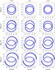 |
Fig. 12 (x,y) projection of the unstable invariant manifolds for the precessing model with Ω = 0.5, GMb ∈ [0.1,0.4] (from top to bottom) and tilt angle ε ∈ [0.,0.2] (from left to right). The position of the equilibrium points is marked with red crosses. |
When Ω = 0.05 (Fig. 12), we observe that the structure of invariant manifolds is preserved for different values of ε, but with small particularities. For example, the position of the invariant manifolds is not exactly the same in the three columns for a given value of GMb. In this way, we can see that the structure remains, but the spiral arms slowly open up. Moreover, when the bar mass increases, the structure moves from a morphology of a rR1 ringed galaxy to the one of a spiral galaxy as expected (Romero-Gómez et al. 2007).
When we increase the pattern speed to Ω = 0.06, we appreciate (in Fig. 13) that, although the basic structure is preserved, the arms are more open even for low bar masses. And again, the behaviour of the manifolds are the same with respect to the variation in ε.
Figures 14 and 15 show the previous panels in three dimensions to better appreciate the variation with respect to the tilt angle of the model. Here, we clearly see the structures that have been discussed before, and we see how the invariant manifolds change in the z component.
In Figs. 16 and 17, we show a possible approach to the evidence of detected warps in galaxies. In a side-on view, and when the tilt angle ε> 0, we observe that the outer branches of the unstable manifold are clearly warped, emulating the shape of some observed galaxies. For example, when we take a bar mass GMb = 0.2, all plots present a warped shape, and differences among them are obtained when one varies the inclination and pattern speed.
For Ω = 0.05 (Fig. 16), we can see that no warped shape appears with ε = 0 as expected. But, when ε is increased, as well as GMb, different warp shapes are present. With GMb = 0.2, invariant manifolds are just hinting at the shape of warps, and when GMb = 0.3, the warps are clearly shown.
The same phenomenon occurs for the pattern speed Ω = 0.06 (Fig. 17). But in this case the warped structure is present for a wider variety of parameter combinations. With ε> 0, a warp is present already with a bar mass of GMb = 0.2. As GMb increases, the S shape of the warp becomes more evident, increasing its inclination with respect to the galactic plane, where the most tilted case is the one with ε = 0.2 and GMb = 0.4. Also, the contribution of the inner branches of the invariant manifolds are more evident with a pattern speed faster than Ω = 0.05.
To get an overall vision, in Fig. 18 we show the invariant manifolds for GMb = 0.3, Ω = 0.05, and ε = 0.2 (hereafter Model S), together with the Ferrers bar and the zero velocity surface of the energy level considered. With this model, we are able to appreciate the strong resemblance with the warp of the Integral Sign Galaxy (Fig. 19).
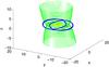 |
Fig. 18 3D view of the unstable invariant manifolds (blue), zero velocity surface (green), and triaxial Ferrers bar (yellow) for Model S. The red crosses indicate the position of the equilibrium points. |
In summary, we conclude that the warp formation is closely related to the pattern speed of the bar, the bar mass and, especially, to the tilt angle of the model, as we expected. We also note that if we consider a symmetric bar instead of a bar with b ≠ c, the results are essentially identical.
4.1. Warp angles
We measure the maximum amplitude of the warp as the angle between the outermost detected point and the mean position of the plane of symmetry, as defined by the internal unwarped region, as in Sánchez-Saavedra et al. (2003). The warp angle obtained in our theoretical analysis varies considerably depending on the pattern speed, bar and disc masses, and above all, the tilt angle ε. As we can observe in Table 1, when the pattern speed increases, the warp angle increases, too. The same phenomenon occurs when we fix a pattern speed and increase the bar mass, but the biggest increment takes place when the tilt angle ε grows. In this context, there are no warps when ε = 0, as expected, but the highest warp angle, θ = 9.3°, is reached when we use the maximum values considered for all the variables. For example, for a pattern speed of Ω = 0.05, the maximum angle obtained is θ = 7.7°, by setting the parameters ε = 0.2, GMb = 0.4, GMd = 0.6. Whereas, if we take a pattern speed of Ω = 0.06 and keep the previous values for the remaining parameters, we obtain a warp angle of θ = 9.3°.
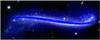 |
Fig. 19 Warp obtained for Model S (blue) superimposed on the Integral Sign Galaxy, UGC 3697. |
The catalogue of warps in the southern hemisphere (Sánchez-Saavedra et al. 2003) shows that most warps have angles less than 11°, which is very close to the maximum warp angle of θ = 9.3° we obtained with our theoretical model. We notice that the tilt angle ε has to be small, since otherwise the system would lose its consistency, in the sense that if the tilt angle were bigger, the model would be unstable, and it would lead to chaotic dynamics. The model is stable up to tilt angles slightly above ε = 0.25 rad, which could produce warp angles close to 11°.
Warp angles (in degrees) obtained in the precessing model.
5. Test particle simulation
The advantage of test particle simulations is that the stars are evolved using a known galactic potential, and they have inherited the information on both density and kinematics, that is, the stars are in statistical equilibrium with the potential imposed after a certain integration time. They are used as generators of mock catalogues (Romero-Gómez et al. 2015) or to obtain information of the potential imposed by studying certain aspects of the simulation, for example the moving groups in the solar neighbourhood (e.g. Dehnen 2000; Fux 2001; Gardner & Flynn 2010; Minchev et al. 2010; Antoja et al. 2011).
The purpose of using test particle simulations here is twofold: to show that the particles are trapped in the manifolds when integrating in the precessing model and present a warped shape, and to show that not only do the manifolds warp, but the orbits in the disc also present a warped shape. The manifolds, which are the backbone of the spiral arms, contribute to it. Therefore, we generate a set of 106 particles using the Hernquist method (Hernquist 1993). The density follows the same Miyamoto-Nagai disc (see Appendix of Romero-Gómez et al. 2015) as in the analytical computations. We give the particles the initial velocity for a circular orbit with zero dispersion. The bar pattern speed is set to Ω = 0.05 [ut]-1; i.e., one bar rotation takes 125 Myr. The bar is introduced adiabatically in t1 = 16 bar rotations, using the same time function as in Dehnen (2000) in the precessing model:  (21)and Ab = 0 if t ≤ 0. Here, Ab grows with time in the interval t ∈ (0,t1) and assumes its maximal amplitude when t ≥ t1, in which Ab = Af; that is, it assumes the total bar amplitude. Since Eq. (21) is continuous and derivable, a smooth transition from umbarred to a barred galaxy is guaranteed.
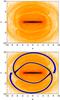 |
Fig. 20 Top: surface density of the xy projection of the test particle simulation for Model S. Bottom: overlap of the invariant manifolds for the same parameters (in blue) with Jacobi constant CJ = −0.19366. |
To keep the total mass of the system constant when we introduce the bar adiabatically, we transfer mass from the disc to the bar progressively, so that  (22)where φT is the total potential of the system, φd, φb the potentials of the disc and bar, respectively, and the time function f(t) is the same polynomial of time t as in Eq. (21). The parameter f0 takes the value of the final bar mass, f0 = GMb = 0.3, so that when the integration time reaches the maximum amplitude of the bar, t = t1, the bar mass is GMb = 0.3 and the mass disc GMd = 0.7. Thus, we consider Model S once the final configuration is reached.
The particles in the xy plane adopt the shape seen in Sect. 4. The top panel of Fig. 20 presents the configuration of the particles, which acquire characteristic features. We observe how some particles are concentrated in the L4 (L5) region, whose stable family of periodic orbits prevents these particles from exiting the region. Even though the L4 and L5 Lagrangian points always remain in the galactic plane, the orbits around them are non-planar, and they contribute slightly to the warped shape. Also, the particles in the outer parts of the zero velocity curves adopt the shape of the invariant manifolds as we expected. This is shown in the bottom panel of Fig. 20, where for the selected model, we overlap the invariant manifolds of the unstable orbits around L1 and L2 with a Jacobi integral CJ close to that of the equilibrium point L1 (CJ = −0.19366 and CJ,L1 = −0.19368).
However, the particles trapped in the manifolds are not all that contribute to warping the disc. In Fig. 21 we show the surface density and its contour levels in the xz projection of the test particle simulation (top panel), and we overlap the invariant manifolds of the unstable orbits around L1 and L2 (bottom panel). We note, first, how the precessing model tilts the bar and disc, and it shows a warped shape towards the outer parts. We also point out the overdensity due to the superposition of the bar and the particles trapped by the outer branches of the invariant manifolds. This overdensity is not only due to the invariant manifolds, since in other models it can be due to other families of periodic orbits that are trapped in the vertical resonances forming a thick spiral (see e.g. Kalnajs 1973; Patsis & Grosbol 1996).
If we compare the density contour with others found in the literature, such as the one shown in Fig. 3 of Debattista & Sellwood (1999) obtained from an N-body simulation, we observe that the tilting of our model is evidently acquiring a similar shape to the one in the mentioned figure. We can also compare our results to those of observations. As previously mentioned, the invariant manifolds of this model match the profile shown by the Integral Sign Galaxy (Fig. 19). In this case, the maximum angle of the warp is θ = 6.7°. This value agrees with warp angles observed in external galaxies (Sánchez-Saavedra et al. 2003), as discussed in Sect. 4.1. Using the test particle simulation, we can see that indeed the particles integrated in the precessing model do indeed get warped in a similar way to the Integral Sign Galaxy.
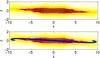 |
Fig. 21 Top: surface density and contours of the xz projection of the test particle simulation for Model S. Bottom: overlap of the invariant manifolds for the same parameters (in blue) with Jacobi constant CJ = −0.19366. |
6. Discussion
Although warps are a common feature in galaxies, there is still no agreement on how the warp is formed. In this paper we continue an idea that started in Romero-Gómez et al. (2006). It is based on the possibility that spirals and rings in barred galaxies are driven by the invariant manifolds associated to the unstable Lyapunov periodic orbits around the unstable equilibrium points in the rotating bar potential. Here we investigate the effect of tilting the model with respect to the XY plane, which is equivalent to a small misalignment between the angular momentum and the angular velocity of the system. Since invariant manifolds behave like tubes transporting matter, we have been able to observe that owing to the small misalignment, these manifolds reproduce warped shapes as observed in warped galaxies. When we study the motion of test particles under the precessing model, we see that even though the main contribution comes from the invariant manifolds, all orbits warp. In addition, we have shown the consistency of the model despite its tilting thanks to the periodic orbits inside the bar (around the central equilibrium point), which continue to be responsible for the bar structure and to constitute its backbone.
To make certain that our principal results do not depend on the model, we prove our theory with a model composed of a bar with revolution symmetry and another one with just axial symmetry. In both models, the periodic orbits around the central point L3 contribute to the backbone of the bar, where the family of periodic orbits are qualitatively the same in both cases, and although the shape of the stability indexes varies, the range of energies in which the orbits are stable is the same. But the main point is that the invariant manifolds in both models are very similar and acquire the same warped form, in the sense that if we take equal values for the free parameters (bar mass, bar disc, tilt angle, and pattern speed), we obtain equivalent warped shapes.
The addition of a spherical dark matter halo to the galactic model has been studied in detail in Sánchez-Martín (2015), where it leads to the same results as in this work. The position of the equilibrium points varies with the presence or absence of the halo and with its mass. But the behaviour of these points does not change: the two equilibrium points at the ends of the bar continue to be unstable, whereas the rest remain stable. As for the invariant manifolds, the halo affects the inner to a greater extent than the outer branches of the invariant manifolds. An increase in the mass of the halo makes the inner branches join and the outer ones to become more open, while if its mass decreases, the inner branches open up, forming a ring, and the outer branches slowly close. The halo also influences the formation of warps, favouring larger warp amplitudes, but within observational ranges.
Compared with observations, we can confirm that the warp angles obtained with this precessing model closely approximate observed warps. We observe that the tilt angle ε, which is the angle between the angular momentum and the angular velocity, is also responsible for the warp shape, though the warped shape also depends on the pattern speed and bar mass, albeit to a second order. We show that if the bar mass grows or the pattern speed is faster, the warp angle increases. In the precessing model, the warp begins close to the corotation radius, where the Lagrangian points are located, and it is related to the warped invariant manifolds. In external galaxies, it is believed that the galaxies are flat within R25, and warps become detectable within the Holmberg radius, RHo = R26.5 (Briggs 1990), which are the radii of the isophote of an elliptical galaxy corresponding to a surface brightness of 25 and 26.5, respectively, blue magnitudes per square arcsecond. It is difficult to test whether the Holmberg radius is close to the corotation radius because there are few edge-on warped galaxies classified as spiral barred galaxies. In some galaxies we can obtain the ratio Rbar/R25, which is 0.1 for NGC 3344 (Verdes-Montenegro et al. 2000), 0.19 for M 33 (Elmegreen et al. 1992; Hernández-López et al. 2009), and 0.37 for NGC 5560 (Baillard et al. 2011). These values indicate that the warp begins far from the end of the bar, but the relation between Rbar and the corotation radius depends on the bar pattern speed. If it is a slow rotator, the corotation radius moves farther out and can be close to R25, or at least within the area the spiral arms cover.
The warps generated in N-body simulations have a different origin from the one proposed here. They include a reorientation of the outer halo caused by cosmic infall (e.g. Jiang & Binney 1999; Shen & Sellwood 2006), a flyby scenario that is caused by an impulsive encounter between two galaxies (Kim et al. 2014), bending instabilities (Revaz & Pfenniger 2004), an external tidal torque causing a tumbling misaligned halo with the disk (Dubinski & Chakrabarty 2009). Such misalignments can also be between the inner disc and the hot gaseous halo (Roškar et al. 2010), between the angular momenta of the disk and halo (Debattista & Sellwood 1999), or between the principal axes of the triaxial halo (Hu & Sijacki 2015). The warps obtained in the works mentioned above have very similar characteristics, and the warp angles obtained are comparable to the ones from observations, although in some cases, the warp angle remains in the lower ranges (e.g. Revaz & Pfenniger 2004; Kim et al. 2014). Not all simulations are cold enough to form non-axisymmetric structures like bar and spiral arms, such as in the cosmological simulation by Roškar et al. (2010); however, in other cases, a spiral structure is present in the outer parts of the disc as well as in the warp (Debattista & Sellwood 1999; Dubinski & Chakrabarty 2009; Kim et al. 2014; Hu & Sijacki 2015). In the recent work of Hu & Sijacki (2015), the authors claim that the warp interferes very little with the spiral structures. This also occurs in our precessing model, where we showed that the XY projection remains the same as if no misalignment between the angular momentum and angular velocity exists. Dubinski & Chakrabarty (2009) show that the disk behaves as a rigid body and that stars in the outer parts of the disc, with weaker self-gravity, are the ones that precess differentially and form the warp.
Finally, let us point out that this work is a first approximation to establish which parameters in our model are related to the formation of warps. A more detailed classification of the warps obtained will be the subject of future investigation.
Acknowledgments
This work has been partially supported by the MINECO (Spanish Ministry of Economy) – FEDER grants AYA2012-39551-C02-01 and ESP2013-48318-C2-1-R, MTM2012-31714 and the Catalan Grant 2014SGR504. P.S.M. has been supported by the Catalan Ph.D. grants FI-AGAUR and FPU-UPC. The test particle simulations were run in the clusters EIXAM (at MA1-UPC) and Sol (at DAM-UB). We thank the anonymous referee for constructive comments that helped improve the manuscript.
References
- Antoja, T., Figueras, F., Romero-Gómez, M., et al. 2011, MNRAS, 418, 1423 [NASA ADS] [CrossRef] [Google Scholar]
- Arnold, V. I. 1989, Mathematical methods of classical mechanics, Graduate Texts in Mathematics (New York: Springer), 60 [Google Scholar]
- Athanassoula, E., Bienaymé, O., Martinet, L., & Pfenniger, D. 1983, A&A, 127, 349 [NASA ADS] [Google Scholar]
- Athanassoula, E., Romero-Gómez, M., & Masdemont, J. J. 2009, MNRAS, 394, 67 [NASA ADS] [CrossRef] [Google Scholar]
- Avner, E. S., & King, I. R. 1967, AJ, 72, 650 [NASA ADS] [CrossRef] [Google Scholar]
- Baillard, A., Bertin, E., de Lapparent, V., et al. 2011, A&A, 532, A74 [NASA ADS] [CrossRef] [EDP Sciences] [Google Scholar]
- Binney, J., Jiang, I.-G., & Dutta, S. 1998, MNRAS, 297, 1237 [NASA ADS] [CrossRef] [Google Scholar]
- Bosma, A. 1981, AJ, 86, 1791 [NASA ADS] [CrossRef] [Google Scholar]
- Briggs, F. H. 1990, ApJ, 352, 15 [NASA ADS] [CrossRef] [Google Scholar]
- Broucke, R. 1969, AIAA J., 7, 1003 [NASA ADS] [CrossRef] [Google Scholar]
- Canalias, E., & Masdemont, J. J. 2006, Discret. Contin. Dyn. S, 14, 261 [Google Scholar]
- Combes, F. 1994, How Galaxies Accrete Mass and Evolve: Spiral Waves and Bars, Warps and Polar Rings, in The Formation and Evolution of Galaxies, eds. C. Muñoz-Tuñón, & F. Sánchez (Cambridge: Cambridge University Press), 317 [Google Scholar]
- Contopoulos, G. 1981, A&A, 102, 265 [NASA ADS] [Google Scholar]
- Contopoulos, G., & Grosbøl, P. 1989, A&ARv, 1, 261 [NASA ADS] [CrossRef] [Google Scholar]
- Contopoulos, G., & Papayannopoulos, T. 1980, A&A, 92, 33 [NASA ADS] [Google Scholar]
- Cox, A. L., Sparke, L. S., Van Moorsel, G., & Shaw, M. 1996, AJ, 111, 1505 [NASA ADS] [CrossRef] [Google Scholar]
- Debattista, V. P., & Sellwood, J. A. 1999, ApJ, 513, 107 [Google Scholar]
- Dehnen, W. 2000, AJ, 119, 800 [NASA ADS] [CrossRef] [Google Scholar]
- Dubinski, J., & Chakrabarty, D. 2009, ApJ, 703, 2068 [NASA ADS] [CrossRef] [Google Scholar]
- Elmegreen, B. G., Elmegreen, D. M., & Montenegro, L. 1992, ApJS, 79, 37 [NASA ADS] [CrossRef] [Google Scholar]
- Ferrers, N. M. 1877, Q. J. Pure Appl. Math., 14, 1 [Google Scholar]
- Fux, R. 2001, A&A, 373, 511 [NASA ADS] [CrossRef] [EDP Sciences] [Google Scholar]
- Gardner, E., & Flynn, C. 2010, MNRAS, 405, 545 [NASA ADS] [Google Scholar]
- Goldstein, H. 1980, Classical Mechanics, 2nd edn. (Addison-Wesley Publishing Company) [Google Scholar]
- Hadjidemetriou, J. D. 1975, Cel. Mech., 12, 255 [NASA ADS] [CrossRef] [Google Scholar]
- Hernández-López, I., Athanassoula, E., Mújica, R., & Bosma, A. 2009, Rev. Mex. Astron. Astrofis., 37, 160 [Google Scholar]
- Hernquist, L. 1993, ApJS, 86, 389 [NASA ADS] [CrossRef] [Google Scholar]
- Hu, S., & Sijacki, D. 2015, MNRAS, submitted [arXiv:1507.01643] [Google Scholar]
- Hunter, C., & Toomre, A. 1969, ApJ, 155, 747 [NASA ADS] [CrossRef] [Google Scholar]
- Jiang, I. G., & Binney, J. 1999, MNRAS, 303, L7 [NASA ADS] [CrossRef] [Google Scholar]
- Kalnajs, A. J. 1973, PASA, 2, 174 [Google Scholar]
- Kim, J. H., Peirani, S., Kim, S., Ann, H. B., An, S.-H., & Yoonm, S.-J. 2014, ApJ, 789, 90 [NASA ADS] [CrossRef] [Google Scholar]
- Levine, E. S., Blitz, L., & Heiles, C. 2006, ApJ, 643, 881 [NASA ADS] [CrossRef] [Google Scholar]
- López-Corredoira, M., Betancort-Rijo, J., & Beckman, J. E. 2002, A&A, 386, 169 [NASA ADS] [CrossRef] [EDP Sciences] [Google Scholar]
- Lynden-Bell, D. 1965, MNRAS, 129, 299 [NASA ADS] [CrossRef] [Google Scholar]
- Minchev, I., Boily, C., Siebert, A., & Bienaymé, O. 2010, MNRAS, 407, 2122 [NASA ADS] [CrossRef] [MathSciNet] [Google Scholar]
- Miyamoto, M., & Nagai, R. 1975, PASJ, 27, 533 [NASA ADS] [Google Scholar]
- Ollé, M., & Pfenniger, D. 1998, A&A, 334, 829 [NASA ADS] [Google Scholar]
- Ostriker, E. C., & Binney, J. 1989, MNRAS, 237, 785 [NASA ADS] [CrossRef] [Google Scholar]
- Patsis, P. A. 2006, MNRAS, 369, L56 [NASA ADS] [CrossRef] [Google Scholar]
- Patsis, P. A., & Grosbol, P. 1996, A&A, 315, 371 [NASA ADS] [Google Scholar]
- Pfenniger, D. 1984, A&A, 134, 373 [NASA ADS] [Google Scholar]
- Read, J. I., Lake, G., Agertz, O., & Debattista, V. P. 2008, MNRAS, 389, 1041 [NASA ADS] [CrossRef] [Google Scholar]
- Revaz, Y., & Pfenniger, D. 2004, A&A, 425, 67 [NASA ADS] [CrossRef] [EDP Sciences] [Google Scholar]
- Romero-Gómez, M., Masdemont, J. J., Athanassoula, E., & García-Gómez, C. 2006, A&A, 453, 39 [NASA ADS] [CrossRef] [EDP Sciences] [Google Scholar]
- Romero-Gómez, M., Athanassoula, E., Masdemont, J. J., & García-Gómez, C. 2007, A&A, 472, 63 [NASA ADS] [CrossRef] [EDP Sciences] [Google Scholar]
- Romero-Gómez, M., Masdemont, J. J., García-Gómez, C., & Athanassoula, E. 2009, Comm. Nonlinear Science Numerical Simulation, 14, 4123 [NASA ADS] [CrossRef] [Google Scholar]
- Romero-Gómez, M., Figueras, F., Antoja, T., Abedi, H., & Aguilar, L. 2015, MNRAS, 447, 218 [NASA ADS] [CrossRef] [Google Scholar]
- Roškar, R., Debattista, V. P., Brooks, A. M., et al. 2010, MNRAS, 408, 783 [NASA ADS] [CrossRef] [Google Scholar]
- Sánchez-Martín, P. 2015, Doctoral Dissertation, http://hdl.handle.net/10803/299366 (Barcelona: Universitat Politècnica de Catalunya) [Google Scholar]
- Sánchez-Saavedra, M. L., Battaner, E., & Florido, E. 1990, MNRAS, 246, 458 [NASA ADS] [Google Scholar]
- Sánchez-Saavedra, M. L., Battaner, E., Guijarro, A., López-Corredoira, M., & Castro-Rodríguez, N. 2003, A&A, 399, 457 [NASA ADS] [CrossRef] [EDP Sciences] [Google Scholar]
- Sellwood, J. A. 2013, Dynamics of Disks and Warps, in Planets, Stars and Stellar Systems, eds. T. D. Oswalt, & G. Gilmore (Dordrecht: Springer), 5, 923 [Google Scholar]
- Shen, J., & Sellwood, J. A. 2006, MNRAS, 370, 2 [NASA ADS] [CrossRef] [Google Scholar]
- Skokos, Ch., Patsis, P. A., & Athanassoula, E. 2002a, MNRAS, 333, 847 [NASA ADS] [CrossRef] [Google Scholar]
- Skokos, Ch., Patsis, P. A., & Athanassoula, E. 2002b, MNRAS, 333, 861 [NASA ADS] [CrossRef] [Google Scholar]
- Sparke, L. S., & Casertano, S. 1988, MNRAS, 234, 873 [NASA ADS] [CrossRef] [Google Scholar]
- Verdes-Montenegro, L., Bosma, A., & Athanassoula, E. 2000, A&A, 356, 827 [NASA ADS] [Google Scholar]
- Voglis, N., & Stavropoulos, I. 2005, in Recent advances in astronomy and astrophysics, ed. N. Solomos, AIP Conf. Proc., 848, 647 [Google Scholar]
- Voglis, N., Stavropoulos, I., & Kalapotharakos, C. 2006, MNRAS, 372, 901 [NASA ADS] [CrossRef] [Google Scholar]
All Tables
All Figures
|
Fig. 1 Galaxy ESO 510-G13 photographed by the Hubble telescope. |
| In the text | |
|
Fig. 2 Reference systems. Top: bar in the body reference frame, where the angular momentum Lb and the ybzb plane keep an angle ε. Bottom: bar in the inertial reference frame, where the angular momentum is aligned with the Z axis and the major axis of the bar keeps an angle ε with the XY plane. |
| In the text | |
|
Fig. 3 Reference systems. The major axis of the bar is aligned with the precessing x axis, and the precessing z axis describes a cone about the inertial Z axis. Here (xp,yp,zp) denotes the precessing reference frame and (X,Y,Z) the inertial one. |
| In the text | |
|
Fig. 4 Rotation curve of the potential φ = φb + φd. |
| In the text | |
|
Fig. 5 Equilibrium points of the precessing model with GMb = 0.1. Top: xy plane with zero velocity curves for a Jacobi constant CJ = −0.1876. Bottom: xz plane, “+” for ε = 0, “×” for ε = 0.1, “•” for ε = 0.2, while the “∗” shows the position of the central L3 point. The blue curve in both panels outlines the triaxial Ferrers bar. |
| In the text | |
|
Fig. 6 Variation of the xz coordinates of L1 as ε varies within the range ε ∈ [0,0.2] for the precessing model with GMb = 0.1. The marked dots show the L1 coordinates for three specific values of ε: ε = 0 (bottom part of the plot), ε = 0.1 (middle), and ε = 0.2 (top). |
| In the text | |
|
Fig. 7 Family of periodic orbits of the precessing model with b ≠ c and GMb = 0.1 (first row: 3D view; second, third, and fourth rows: (x,y), (x,z), and (y,z) projections, respectively) and stability indexes (bottom row) for ε = 0,0.1,0.2 (left, middle and right columns, respectively). In the first four rows, the red dashed lines outline the position of the triaxial Ferrers bar, while the blue lines are periodic orbits of the precessing model. In the bottom row: dark magenta (brown) lines indicate the b1 (b2) stability index. |
| In the text | |
|
Fig. 8 Family of periodic orbits of the precessing model with b ≠ c for ε = 0 (blue) and ε = 0.2 (purple) and GMb = 0.1. From top to bottom: 3D view, xz-plane (left), yz-plane (right). Red (green) lines show the position of the bar for ε = 0 (ε = 0.2). Blue (purple) lines indicate the periodic orbits of the model for ε = 0 (ε = 0.2). |
| In the text | |
|
Fig. 9 Family of periodic orbits of the precessing model with b = c = 0.95 and GMb = 0.1 (first row: 3D view; second, third, and fourth rows: (x,y), (x,z), and (y,z) projections, respectively) and stability indexes (bottom row) for ε = 0,0.1,0.2 (left, middle, and right columns, respectively). In the first four rows, the red dashed lines outline the position of the triaxial Ferrers bar, while the blue lines are periodic orbits of the precessing model. In the bottom row: dark magenta (brown) lines indicate the b1 (b2) stability index. |
| In the text | |
|
Fig. 10 Lyapunov family of periodic orbits around L2 for the model with GMb = 0.1 and for a range of values of the Jacobi constant in (CJ,L2,CJ,L2 + 2 × 10⁻³), where CJ,L2(ε = 0) = −0.1879, CJ,L2(ε = 0.1) = −0.1876 and CJ,L2(ε = 0.2) = −0.1865. The tilt angle ε ∈ [0,0.2]. Note the varying scale of the vertical axis. |
| In the text | |
|
Fig. 11 Stable and unstable invariant manifold associated to the periodic orbit around L1 with ε = 0.2 and GMb = 0.3. |
| In the text | |
|
Fig. 12 (x,y) projection of the unstable invariant manifolds for the precessing model with Ω = 0.5, GMb ∈ [0.1,0.4] (from top to bottom) and tilt angle ε ∈ [0.,0.2] (from left to right). The position of the equilibrium points is marked with red crosses. |
| In the text | |
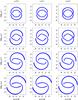 |
Fig. 13 As in Fig. 12 for Ω = 0.06. |
| In the text | |
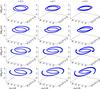 |
Fig. 14 As in Fig. 12 in a 3D view. |
| In the text | |
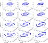 |
Fig. 15 As in Fig. 13 in a 3D view. |
| In the text | |
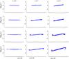 |
Fig. 16 As in Fig. 12 but in the side-on view. |
| In the text | |
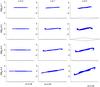 |
Fig. 17 As in Fig. 13 but in the side-on view. |
| In the text | |
|
Fig. 18 3D view of the unstable invariant manifolds (blue), zero velocity surface (green), and triaxial Ferrers bar (yellow) for Model S. The red crosses indicate the position of the equilibrium points. |
| In the text | |
|
Fig. 19 Warp obtained for Model S (blue) superimposed on the Integral Sign Galaxy, UGC 3697. |
| In the text | |
|
Fig. 20 Top: surface density of the xy projection of the test particle simulation for Model S. Bottom: overlap of the invariant manifolds for the same parameters (in blue) with Jacobi constant CJ = −0.19366. |
| In the text | |
|
Fig. 21 Top: surface density and contours of the xz projection of the test particle simulation for Model S. Bottom: overlap of the invariant manifolds for the same parameters (in blue) with Jacobi constant CJ = −0.19366. |
| In the text | |
Current usage metrics show cumulative count of Article Views (full-text article views including HTML views, PDF and ePub downloads, according to the available data) and Abstracts Views on Vision4Press platform.
Data correspond to usage on the plateform after 2015. The current usage metrics is available 48-96 hours after online publication and is updated daily on week days.
Initial download of the metrics may take a while.