| Issue |
A&A
Volume 588, April 2016
|
|
|---|---|---|
| Article Number | A103 | |
| Number of page(s) | 26 | |
| Section | Catalogs and data | |
| DOI | https://doi.org/10.1051/0004-6361/201525648 | |
| Published online | 24 March 2016 | |
Second ROSAT all-sky survey (2RXS) source catalogue⋆
Max-Planck-Institut für extraterrestrische Physik, 85748 Garching, Giessenbachstraße, Germany
e-mail: This email address is being protected from spambots. You need JavaScript enabled to view it.
Received: 8 January 2015
Accepted: 29 February 2016
Abstract
Aims. We present the second ROSAT all-sky survey source catalogue, hereafter referred to as the 2RXS catalogue. This is the second publicly released ROSAT catalogue of point-like sources obtained from the ROSAT all-sky survey (RASS) observations performed with the position-sensitive proportional counter (PSPC) between June 1990 and August 1991, and is an extended and revised version of the bright and faint source catalogues.
Methods. We used the latest version of the RASS processing to produce overlapping X-ray images of 6.4° × 6.4° sky regions. To create a source catalogue, a likelihood-based detection algorithm was applied to these, which accounts for the variable point-spread function (PSF) across the PSPC field of view. Improvements in the background determination compared to 1RXS were also implemented. X-ray control images showing the source and background extraction regions were generated, which were visually inspected. Simulations were performed to assess the spurious source content of the 2RXS catalogue. X-ray spectra and light curves were extracted for the 2RXS sources, with spectral and variability parameters derived from these products.
Results. We obtained about 135 000 X-ray detections in the 0.1−2.4 keV energy band down to a likelihood threshold of 6.5, as adopted in the 1RXS faint source catalogue. Our simulations show that the expected spurious content of the catalogue is a strong function of detection likelihood, and the full catalogue is expected to contain about 30% spurious detections. A more conservative likelihood threshold of 9, on the other hand, yields about 71 000 detections with a 5% spurious fraction. We recommend thresholds appropriate to the scientific application. X-ray images and overlaid X-ray contour lines provide an additional user product to evaluate the detections visually, and we performed our own visual inspections to flag uncertain detections. Intra-day variability in the X-ray light curves was quantified based on the normalised excess variance and a maximum amplitude variability analysis. X-ray spectral fits were performed using three basic models, a power law, a thermal plasma emission model, and black-body emission. Thirty-two large extended regions with diffuse emission and embedded point sources were identified and excluded from the present analysis.
Conclusions. The 2RXS catalogue provides the deepest and cleanest X-ray all-sky survey catalogue in advance of eROSITA.
Key words: X-rays: general / catalogs / surveys
The catalogue is only available at the CDS via anonymous ftp to cdsarc.u-strasbg.fr (130.79.128.5) or via http://cdsarc.u-strasbg.fr/viz-bin/qcat?J/A+A/588/A103
© ESO, 2016
1. Introduction
The ROSAT all-sky survey (RASS) was the first to scan the whole sky with a powerful imaging X-ray telescope operating in the 0.1−2.4 keV band (Trümper 1982). The Wolter type I mirror system (Aschenbach 1988) was exceptionally well suited for the sky survey operation because of the very low micro-roughness of the mirrors (<0.3 nm), which was responsible for the excellent contrast of the X-ray images. The focal plane detector used for the sky survey, the position-sensitive proportional counter (PSPC), had a five-sided anti-coincidence system that reduced the particle background with an efficiency of 99.85% (Pfeffermann & Briel 1986; Pfeffermann et al. 2003). This efficient anti-coincidence veto design resulted in a low, non-X-ray (particle) background. Another reason for the exceptionally low particle background of ROSAT was the low Earth orbit with orbital height of ~ 580 km and inclination 53° (orbital period 96 min).
The ROSAT survey observations were performed in scanning mode, where the field of view (FOV) of the PSPC detector scanned a two-degrees-wide strip along a great circle over the ecliptic poles within 96 min. With a shift of about one degree per day, an all-sky survey was completed within half a year. Because of periods of very high background or poor attitude values, some parts of the sky were missed, but re-observed during the February survey in 1991 and the August survey in 1991. Before the main survey between August 1990 and January 1991, the July mini-survey in 1990 was performed for testing and is part of the ROSAT all-sky survey. Still some parts of the sky remained unobserved, which were later (February 1997) covered by pointing observations. The analysis of these will be reported in a separate paper (Freyberg et al., in prep.).
The RASS sensitivity (Trümper 1993) surpassed that of the Uhuru (Forman et al. 1978) and HEAO-1 (Wood et al. 1984) surveys by a factor >100 in the soft X-ray band. The RASS bright source catalogue (RASS BSC), containing 18 806 sources, was first published in electronic form (Voges et al. 1996) and later in a printed version (Voges et al. 1999). This catalogue has served a very large scientific community working in different fields – from solar system objects (Moon, comets, and planets) out to clusters of galaxies and quasars at large cosmological distances. The faint part of the ROSAT all-sky survey (RASS FSC) with 105 924 sources down to a detection likelihood limit of 6.5 was published only in an electronic version (Voges et al. 2000). Both RASS BSC and FSC, which taken together constitute the ROSAT 1RXS catalogue, were based on the so-called RASS-2 processing (Voges et al. 1999). An updated version of the processing (RASS-3) was performed subsequently with event files being made public, but without further documentation.
After the all-sky survey, ROSAT performed an extended program of pointed observations that covered a significant part of the sky (~ 18%) with deeper observations. Several other satellite missions with imaging telescopes have gathered data over large areas of the sky, producing large catalogues of X-ray point sources. Of particular note are the ROSAT PSPC pointed catalogue (ROSAT Collaboration 2000), the XMM-Newton catalogue of pointed observations (Webb & XMM-Newton Survey Science Centre 2014), the XMM-Newton slew survey (Saxton et al. 2008), and the deep Swift X-ray telescope point source catalogue (Evans et al. 2014).
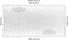 |
Fig. 1 Structure and numbering scheme of the sky fields in the ROSAT all-sky survey in equatorial coordinates (courtesy K. Dennerl, available at the 2RXS web site.) Areas around the North and South ecliptic poles with 1° and 15° radius are indicated at the upper left and lower right corner. |
The aim of this paper is to present a revised point source data base of the ROSAT all-sky survey (ROSAT 2RXS). The main points of improvement are as follows:
-
1.
Use of an improved detection algorithm.
-
2.
Reduction of systematic time delays between star tracker and photon arrival time.
-
3.
A significantly improved reduction of spurious detections by a careful visual screening of each catalogue entry and the exclusion of large, extended emission regions, in particular from the background-map creation process.
-
4.
The provision of X-ray images of 1378 sky fields (6.4° × 6.4°) covering the whole sky.
-
5.
The provision of local maps (40′ × 40′) for each detected X-ray source.
-
6.
The creation of source spectra and light curves and deduction of characteristic parameters.
-
7.
The creation of new photon event tables through correcting astrometric errors that are present in the publicly available event files (originating from the RASS-3 processing).
-
8.
The delivery of a documented and reproducible point source catalogue.
-
9.
Performing extensive simulations to estimate the amount of spurious detections in the 2RXS catalogue as a function of the detection likelihood and other source parameters.
The total number of entries listed in the 2RXS catalogue is 135 118. Of these, 5926 have been flagged as uncertain detections (cf. Sect. 3.2). We have also provided the results of cross correlations of the catalogue with major source catalogues from X-rays and other wavelength bands (see Sect. 6).
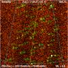 |
Fig. 2 Example for a source count image of sky field 930304 in the way it is used for source detection. For the colour representation in this and all following images the ESO/MIDAS colour table heat is used with linear intensity scaling. The cyan solid lines confine the 6.4° × 6.4° field and the scan direction is marked with the yellow line through the centre of the field. 2RXS sources are indicated with green circles. Detections that were manually flagged as being uncertain (see Sect. 3) are marked with cyan crosses. Coordinates refer to the image centre, the exposure time is the median over the whole image. |
2. 2RXS – data analysis
In the following we describe how the 2RXS catalogue was created (Sect. 2.1 and Appendix A) and how new data products were produced (Sect. 2.2).
2.1. Detection algorithm
We used the data from the third processing of the ROSAT All-Sky Survey (RASS-3) as input, which is publicly available from the MPE ROSAT archival FTP site1: sequences 93nnmmp, with nn ranging from 01 to 33, from the equatorial North Pole in 5.625° steps to the equatorial South Pole, that is, 17 containing the equatorial plane), and mm from 1 to a maximum of 64 (depending on Declination), dividing the equatorial rings along Right Ascension, and prefix 93 being the year of the RASS-2 processing2. The field structure and numbering scheme are illustrated in Fig. 1. Data are thus organised into 1378 overlapping equatorial sky regions of size 6.4° × 6.4°, with event lists originating from the RASS-3 processing.
The RASS-3 processing differs in two points from the RASS-2 processing, which was used to create the 1RXS catalogue. Firstly, the time resolution for the interpolation of the attitude solution (which is given with 1 s accuracy) was refined from 1/64 s to 1/32 000 s. A time delay exists between attitude time and photon time, which is given with a precision of 10 ms. Therefore, a systematic uncertainty of ± 5 ms translates into a systematic positional error (still) in the RASS-3 processing of at least ± 1″ along scan direction. Secondly, in the RASS-3 processing the required number of identified guide stars in the star tracker field to accept photons was relaxed with respect to the RASS-2 processing. This resulted in a larger sky coverage in the RASS-3 processing.
The several phases of the ROSAT all-sky survey (and its completion) are described in a separate paper (Freyberg et al., in prep.). Here we only used data that had been taken in scanning mode during four phases: the mini survey, the main survey, the February survey 91, and the August survey 91 (see Table 2 of Voges et al. 1999).
Periods where the PSPC FOV passed over the Moon (Freyberg 1994) were almost completely removed during RASS-3 processing (remaining periods were excluded in this paper). The photons were rejected from the event lists but kept in separate files.
As for 1RXS, the source detection scheme was optimised to a survey scanning mode with the PSPC and was performed using a three-step approach. The first two steps are based on a sliding cell method, estimating the background locally, and then using background from a model fit. Finally, the resulting source candidate lists are used as input to a maximum likelihood algorithm (for more details see Appendix A). Similar techniques are used for the XMM-Newton catalogues (Watson et al. 2009) and the 1SXPS Swift-XRT catalogue (Evans et al. 2014). However, for the ROSAT survey, likelihood values are determined on an event basis, while the XMM-Newton and Swift methods use binned images. In the ROSAT method the appropriate point-spread function (PSF) and vignetting corrections are assigned to each event: in scanning mode photons from an individual source are detected at very different places in the detector in contrast to a pointed observation, while in the latter (image approach) only an average PSF can be used. In contrast to CCD-type observations, the PSPC does not suffer from so-called out-of-time events such as hot pixels, bad columns, or read-out streaks. Additionally, the highly effective anti-coincidence procedure resulted in a very low particle background. Moreover, the scanning mode smears out remaining telescope artefacts such as stray-light that is due to single reflected X-rays in a Wolter-I telescope. Therefore, we continued with using the ROSAT source detection software, but included several improvements.
Primary source parameters (see Boese 2004) resulting from the source detection procedure are for instance the detection likelihood, exposure time, source counts, count rate, and source extent (with corresponding uncertainties). Derived source parameters include hardness ratios, spectral fit, and variability parameters (with corresponding uncertainties). Cross-correlations with selected catalogues are described in Sect. 6.
The main improvement in the new detection procedure was to use nine smaller overlapping images (2.27° × 2.27°) within the 6.4° × 6.4° sky field instead of only one large image, as used in the second processing of the ROSAT all-sky survey data (see Fig. A.1). As shown by Freyberg (1994), variations in the background and the exposure create intensity structures in the count intensities with typical sizes of about two degrees perpendicular to the scan paths. These variations can be seen in the 6.4° × 6.4° images used for source detection in the 1RXS processing. The background maps produced from spline fits often did not follow these variations, leading to over- or underestimated background in different areas. To overcome this problem, we divided the images into nine (three by three) sub-images. With this smaller sky-field map structure we can better account for the count intensity variations and can better constrain the background for sources. This results in a more precise determination of the detection likelihood values, especially for faint 2RXS sources. In the RASS FSC catalogue about 12 000 detections have artificially high likelihood values that are due to an underestimation of the background resulting from a background map that is not adequately adapted to the count intensity variations present in the ROSAT all-sky survey. In the 2RXS processing these are either absent from the seed source lists or assigned likelihoods below the acceptance threshold and therefore absent from the 2RXS catalogue. This is described in detail in Sect. 4.1.
2.2. Data products
In addition to the source properties obtained by the detection algorithm, higher-level data products were created to allow a more detailed scientific exploration of the 2RXS catalogue. We wrote shell scripts, which call the necessary MIDAS/EXSAS programs in order to produce X-ray images, light curves, and spectra. The data products were produced for all detections above a likelihood of 6.5 identified in the 1378 individual fields covering the ROSAT all-sky survey. The screening procedures applied to all 2RXS sources and larger complex regions are described in Sect. 3.
2.2.1. X-ray images of the 1378 sky fields
We have produced X-ray images in the 0.1−2.4 keV band for each individual sky field with a size of 6.4° × 6.4°. Figure 2 shows the source count image for field 930304. 2RXS sources are marked with green circles, and sources that were manually flagged (see Sect. 3) are shown as cyan crosses. The yellow line indicates the scan path (ecliptic great circle) across the centre of the field. The variations in the count intensities are caused by variations in the background intensity and in the exposure time (Freyberg 1994). The 1378 sky fields with the 2RXS sources overlaid, as well as all the other data products listed below, can be accessed at the catalogue web site3.
2.2.2. X-ray source images
In addition to the 1378 sky field images, we produced zoomed X-ray images with a size of 40′ × 40′ centred on each of the point sources for each of the six energy bands we used in our analysis (see the Appendix for details). Five equally spaced contour lines were determined linearly between the minimum and maximum photon surface density and overlaid on the X-ray images. Figure 3 gives an example for the source 125 in field 930101. The 2RXS sources are marked with green circles, and cyan crosses denote detections that were visually screened and flagged (cf. Fig. 3).
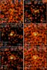 |
Fig. 3 Example of X-ray count rate images for our six energy bands with overlaid X-ray intensity contours (black lines), bands 1 to 6 are defined as PSPC channels 11−41, 52−90, 91−201, 11−235, 52−201, 11−201, respectively (with one channel ~ 10 eV). Each image is centred on source 125 for which the 2RXS IAU name is provided. The broad-band source count rate (PSPC channels 11−235) with error as determined from the detection algorithm is in units of counts ks-1. Contour levels are in units of counts ks-1 arcmin-2. At the top of the image the field number (SeqID) and the source identification within the field (srcID) are given. The green circles gives the catalogue entries, and the cyan cross marks a source that was visually flagged in the screening process. |
2.2.3. X-ray light curves
To create light curves for ROSAT observations in scanning mode, we developed a set of scripts that take all necessary functionality into account and appropriately handle the detector and instrument behaviour, for example, the removal of source scans when the detector was switched off, counting photons when the source is completely in the FOV.
Background extraction regions were taken from two circles along the scan direction with radii of 5′, and separated by a distance of + 30′ and −30′ from the source position. This results in a time offset between the source and background events of eight seconds. On this relatively short time scale, variations in the background are expected to be small, and this approach minimises the effect of these variations. Incorrect background subtraction can occur because previous or following scans contribute, separated by the scan period of 5760 s. When background regions overlap with other sources, we corrected for the fraction of overlap, making sure to use source-free background regions.
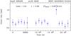 |
Fig. 4 X-ray light curve of 2RXS J043339.0+741012. The mean count rate, the corresponding standard deviation (both in counts s-1), and the normalised excess variance with 1σ uncertainty are given. |
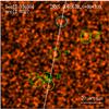 |
Fig. 5 Example of a control image demonstrating how the background region is selected. The background regions for source 27 are shown in cyan (at the top) and yellow circles (at the bottom). Since the yellow circle is contaminated with another source (33), the background in the cyan circle is used in the background subtraction. |
In some of the ROSAT observations (0.9 per cent of the catalogue entries) individual bins have very low exposure values, below 6 s. Such data points are associated with an extreme large error and the calculation of the standard deviations leads to improper values. We have therefore flagged such light curves.
We finally selected the background from the region that is spatially less contaminated by other sources, for an example see Fig. 5.
In the control images the selected background regions are marked with circles in cyan. The source and background light curves were created with a time binning of 11 520 s (corresponding to two orbits). The light curves are provided as plots for each source showing the background-subtracted count rates versus time. We also produced a graph with the number of source and background counts, respectively.
From the light curves we extracted basic parameters, such as the mean count rate, standard deviation, and the minimum and maximum count rate, together with their corresponding errors. To characterise variability, we computed the excess variance with its uncertainty and the maximum amplitude variability as described in Sect. 7.3.4. In Sect. 7.3 we discuss the general timing properties of the 2RXS objects. Figure 4 shows an example light curve for the source with number 48 in the field 930405.
2.2.4. X-ray spectra
We extracted spectra using the same source and background regions as for the light curves. The spectral analysis with three standard models is described in Sect. 7.4. In Fig. 34 an example for a source spectrum with the three model fits is presented.
3. Screening of the second RASS catalogue
3.1. Screening for large extended regions
First we inspected all 1378 ROSAT sky fields for large extended regions with diffuse emission and embedded point sources. In Appendix C we list the sky fields in Table C.2, where we have identified these regions. We give the equatorial coordinates of the source we attribute to large extended regions, and we supply a source identification whenever possible. Sources within the masked regions were excluded from the present 2RXS catalogue. The analysis of point-like X-ray sources within these masked regions will be performed in a subsequent paper (Freyberg et al., in prep.) as further 2RXS sources.
3.2. Visual screening of the 2RXS sources
The number of detections in the 2RXS catalogue with a detection likelihood greater than or equal to 6.5 is 135 118. We visually inspected all the 2RXS sources to confirm their existence and to identify false detections, particularly in the vicinity of bright sources (see, e.g., detection 167 in lower panel of Fig. 6). A simple graphical user interface (GUI) based on a MIDAS/EXSAS script was used to run through all sources. The script creates an image with the source to be validated located at the centre. The image size is 1° by 1°, which allows a zoomed view to the central source and the neighbouring objects. The image shows the X-ray photon surface density with overlaid source detections. By comparing the photon density distribution with the source positions derived from the 2RXS detection algorithm, correct and uncertain detections can be identified. A correct detection is defined by having the source position on top of the maximum value of the photon density distribution.
Using the GUI, we set flags for questionable detections, whereas correct source identifications were marked with the flag SFLAG=0. The top panel of Fig. 6 shows an example of a secure detection. For highly uncertain detections we attributed the flag SFLAG=1. The lower panel of Fig. 6 shows an example of such a case. We flagged 5926 2RXS detections in total.
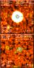 |
Fig. 6 Top: example of a source that is considered as a correct detection, i.e. the source flag is set to zero. The broad-band image is shown. The object is identified as white dwarf WD 1501+663. Bottom: example of an uncertain detection (number 167), located to the lower left of the bright central source (number 164). It is flagged and marked in the image with a cyan cross. Again the broad-band image is shown. |
3.3. Screening statistics
In Fig. 7 we show the distribution of flagged detections normalised to the total number as a function of the exposure time.
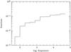 |
Fig. 7 Relative distribution of the 5926 flagged detections as a function of the exposure time. |
With respect to the exposure time distribution, the number of flagged detections increases with exposure time from 1 to 10 per cent above 100 s of exposure time. The reason for this is the very high exposure around the North and South Ecliptic Poles. This leads to an increasing number of uncertain detections when approaching the confusion limit, as the detection software is not optimised for very high source densities. The number of flagged detections with exposure times greater than 10 000 s is 54.
4. 2RXS – 1RXS comparison
The 1RXS catalogue consists of the bright source catalogue (BSC), containing 18 806 sources (Voges et al. 1999), and the faint source catalogue (FSC), containing 105 924 sources (Voges et al. 2000). These are 124 730 sources in total. The number of sources in the 2RXS catalogue without any manual screening flag set is 129 192.
4.1. Detection statistics and detection validation
In Fig. 8 (upper panel) we show the differential and cumulative distributions for the existence likelihood for the 2RXS (in blue) and the 1RXS (red) catalogue entries. In the 2RXS catalogue the lower limit for the existence likelihood is 6.5, which is equivalent to the rounded (nearest integer) value of 7 in the 1RXS catalogue. We note that in the 1RXS catalogue an additional constraint of at least six counts is present, and therefore especially the lowest likelihood bin is affected. From the differential distribution, it is evident that there are more 1RXS detections at the low likelihood end (see inset). Two aspects might account for this: it could be produced by a higher fraction of spurious detections in 1RXS, but also by differing detection likelihood values (cf. Fig. 11 in Sect. 4.2). The second panel of Fig. 8 gives the distributions in count rates. In the range between 0.1 and 1 counts s-1, the differential and integral distributions can be fit with a slope of −2.36 and −1.33, respectively. Both slopes are consistent within the errors (± 0.04). The slopes agree with the log N−log S distribution of AGN (Hasinger et al. 2001). However, in the BSC catalogue, the fraction of stars and extragalactic sources are similar; this may reflect what we see from the 2RXS as a whole.
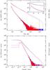 |
Fig. 8 Upper panel: distribution of the detection likelihood values for the 2RXS catalogue (blue) and the 1RXS catalogue (red). The inset shows a zoom to the low-likelihood regime. Lower panel: distribution of count rates for the 2RXS and 1RXS catalogue. Solid and dashed lines denote differential and integral distributions, respectively. The scale for left and right y-axes is identical for all figures with differential and integral distributions. |
To further investigate the differences in the 1RXS and 2RXS detection algorithms, we have compared the background counts for 1RXS and 2RXS sources (Fig. 9). While for a number of sources the background values from the two catalogues are consistent and follow the one-to-one relation, there are sources with significantly higher background values in the 2RXS catalogue. The sources with the largest background offset are located around the poles, where extreme intensity peaks exist, which in turn leads to a large underestimation of the background in 1RXS. The objects on the one-to-one line and the objects located on the middle strip seen in Fig. 9 are randomly distributed over the entire sky, with the exception of the polar regions. Underestimating the background in high-intensity areas leads to an overestimation of the detection likelihood in the 1RXS catalogue. Therefore, the probability that the source is spurious becomes significantly higher for detections with low likelihood values in the 1RXS catalogue. The total number of 2RXS sources that have 1RXS counterparts and defined background ratios is 89 648. The number of sources located at the one-to-one line is 80 753. The object numbers on the strip parallel to the one-to-one line is 7614 (background ratios between greater than 1.2 and lower than or equal to 3.0). The number of objects in the Ecliptic Pole Regions (vertical distribution with respect to the 1RXS background) is 1281 (background ratios greater than three).
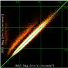 |
Fig. 9 Intensity image of the 2RXS background values on the y-axis versus the 1RXS background values on the x-axis. While most of the objects are located close to the one-to-one line, two other regions are identified (one parallel to the one-to-one line, and a third vertical distribution where most of the objects are located in the ecliptic poles). |
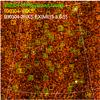 |
Fig. 10 Illustrative comparison of 1RXS (yellow boxes) and 2RXS detections (green circles) for the field 930 304. The image shows the intensity distribution in counts. Perpendicular to the scan directions the count rate shows intensity variations. At the intensity peaks many 1RXS detections do not have an 2RXS counterpart. As the detection algorithm for the 1RXS sources is run on a much larger field size (6.4° by 6.4°), the background at the intensity peaks is often underestimated and the detection likelihood of the sources is overestimated. For the 2RXS sources the detection is run on nine subfields. With this the detection algorithm can much better follow the count rate variations and the background is determined more precisely. At the intensity peaks the background is higher for 2RXS sources and fewer 2RXS sources are detected than at 1RXS. With the white crosses we show 2RXS detections down to likelihood values of 5.5. Some of the 1RXS detections do have an 2RXS counterpart when the likelihood is decreased to 5.5. |
We show the 1RXS and the 2RXS detections as an example for the different detection algorithms applied for the 1RXS and the 2RXS catalogue in Fig. 10 for field 930 304. Here we included those 1RXS detections that do not have a 2RXS counterpart down to the 2RXS existence likelihood limit of 6.5, but have a 2RXS counterpart down to a likelihood limit of 5.5 (marked with white crosses in Fig. 10).
4.2. Comparison of 1RXS and 2RXS detection likelihood distributions
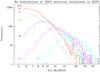 |
Fig. 11 Distribution of 2RXS detection likelihoods for catalogue entries common in both 1RXS and 2RXS for selected 1RXS detection likelihood values of 7 (black dotted), 8 (red solid), 10 (green short-dashed), 12 (blue dash-dotted), 15 (magenta long-dash), and 20 (cyan dash-dotted-dotted). For details see text. |
In Fig. 11 we show the distribution of 2RXS detection likelihoods for catalogue entries common in 1RXS and 2RXS for selected 1RXS detection likelihood values of 7, 8, 10, 12, 15, and 20. It is important to note that the distributions are not delta functions but are rather broad with an extended tail to higher likelihood values. Furthermore, the peak of the 2RXS distribution is below the 1RXS reference value, but the mean is quite similar (e.g., for EXI_ML_1RXS = 12 the mean EXI_ML_2RXS is 11.6). Therefore different threshold effects in 1RXS and 2RXS are expected that for instance lead to missing and new sources, respectively. This plot shows that detection likelihood values obtained with different algorithms cannot be directly compared.
10 096 entries in our detection runs with likelihood values between 5.5 and 6.5 are within 1 arcmin of an 1RXS source and 47 832 detections in this likelihood range do not have a (close-by) 1RXS counterpart. These common detections will also be made available, with a reduced set of information compared to the main catalogue. We regard these common detections as more reliable than other low-likelihood detections in either 1RXS or 2RXS.
4.3. Bright sources in 1RXS and 2RXS
While the 1RXS catalogue contained 18 806 sources according to the selection criteria, the number of 2RXS bright sources determined by applying the same criteria is 22 228. The main reason is that some sources in 1RXS are overestimated in their count rates because the background subtraction is underestimated. If we change the BSC count rate criterion from 0.05 to 0.058 counts s-1 and leave the detection likelihood threshold and number of counts (15 for both catalogues) unchanged, the number of 2RXS bright sources is 18 912, which is similar to the 1RXS BSC. Another effect is the re-distribution of 1RXS detection likelihoods with respect to 2RXS, as shown in Fig. 11. The magenta dashed curve shows the 2RXS detection likelihoods for 1RXS sources with a likelihood of 15. This distribution is very broad, meaning that the detection likelihoods in 1RXS range from 2RXS detection likelihoods from about 5.5 up to 30, with a significant fraction below 15. On the other hand, the blue curve for 1RXS likelihoods of 12 also extends beyond 15, which means that “new” bright sources formally not part of the BSC would now match the criterion.
4.4. Reliability of 2RXS sources with low existence likelihood
4.4.1. Simulations
Fraction of spurious detections.
We performed simulations for the ROSAT all-sky survey to estimate the reliability of the 2RXS catalogue at its faint end. Watson et al. (2009) have pointed out that in 3XMM the relation between the existence likelihood and the detection probability requires calibration through simulations. Similarly, Evans et al. (2014) have performed this analysis for the Swift-XRT 1SXPS catalogue.
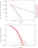 |
Fig. 12 Upper panel: differential (solid blue) distribution of the number of spurious detections and differential (solid red) distribution of catalogue sources. The integral distributions of spurious detections (thin blue, dashed) and catalogue sources (thin red, dashed) are shown in addition with the labelling given on the right y-axis. The solid black thin line gives the theoretical differential relation between the detection likelihood and the probability that a source is spurious. Lower panel: fraction of spurious detections as a function of the existence likelihood. Details of the simulations are described in Sect. 4.4.1. |
To keep all spatial background structures that are due to cosmic and non-cosmic emission, we have used a specific approach. First, we sorted the detection list (down to the limit of EXI_ML = 5.5) for each sky field that does not contain masked regions in increasing order of count rate. For each detection we then determined the fraction of background photons and source photons within the source extraction circle from parameters obtained in the detection run, and correspondingly assigned a probability that a photon is a background photon. If a photon is covered by more than one source extraction region, then the probability is overwritten by subsequent brighter sources. “Source” photons are then statistically removed within the extraction radius, such that the background is flat on scales larger than the source extraction radius (i.e. several arcmin), while all large-scale structures (on scales of degrees) remain unaffected. The remaining photons are then randomly redistributed within the actual field of view at the photon arrival time. This preserves the spatial and temporal structure of the background. Finally, the last step was performed ten times for each of the RASS sky fields without masked emission regions, and the detection algorithm was run identically to the actual observations (see Sect. 2.1). The results are shown in Fig. 12 and Table 1. To our knowledge, this is the first time that such extensive and realistic simulations were performed for ROSAT all-sky survey point source detections.
The solid thin black line in Fig. 12 (upper panel) represents the theoretical relation between the probability P that a source is spurious as a function of the detection likelihood EXI_ML, that is, P = exp(−EXI_ML). This relation refers to the detection likelihood per detection cell. To calculate the differential number of spurious detections, we have to multiply this by the number of detection cells in the ROSAT all-sky survey, if known a priori. Here this number was determined to match the simulated distribution of spurious sources for likelihood values exceeding 10 (see Sect. A.11). For lower likelihood values the theoretical curve is slightly below the differential distribution of spurious detections. This may be due to incompleteness of the input candidate lists to the ML source detection runs in the low-likelihood regime.
Our simulation approach differs from the 2XMM (Watson et al. 2009) and Swift (Evans et al. 2014) simulations of spurious detections. In this paper we have cut out all detections, while in the XMM and Swift approaches the simulated images still include simulated sources. Typical CCD detector features present in pointed observations, such as hot pixels or columns, read-out streaks, or single reflection rings, are not relevant in PSPC scanning mode observations because they either do not exist or are smeared out to an additional large-scale background. Therefore we only have to consider purely statistical spurious sources. As all detected “real” sources have been removed before the simulations, we regard all remaining detections from our simulated data as “spurious”. Most of the systematic artefacts that are due to bright sources have been cleaned by our visual screening procedure because the visual screening flag setting is a human and subjective process.
With this work we are able to quantify the number of spurious detections and for a given detection likelihood value estimate the mean fraction of spurious detections.
The acceptable ratio of real sources to spurious detections is strongly dependent on the scientific application. We choose to release the catalogue down to a likelihood limit of 6.5, which corresponds to the same limit as the ROSAT FSC. This allows users to search for (real) X-ray emission down to very faint limits, but results in a high percentage of detections, mostly at low likelihoods, which are likely to be spurious. Specifically, our estimates show that around 30% of the sources in the entire 2RXS catalogue could be spurious down to this limit. If a lower spurious fraction is considered important by the user, a higher likelihood threshold can be chosen to generate a more reliable catalogue. To give some examples, the likelihood threshold and the integral spurious numbers for existence likelihood values of 20, 10, 5, 2, and 1 per cent are EXI_ML = 6.96, 22602 sources (20% spurious), EXI_ML = 8.08, 8547 sources (10%), EXI_ML = 9.03, 3517 (5%), EXI_ML = 10.18, 1189 (2%), and EXI_ML = 11.01, 533 (1%), respectively. In Fig. 14 we show the cumulative fraction of spurious detections as a function of detection likelihood.
The fraction of spurious detections depends on the number of “real” sources per field, which means that fields with high object numbers possess a lower fraction of spurious detections because the mean number of spurious detections does not depend on the number of catalogue sources in the field (this holds only for our simulation approach with cutting out all sources before the simulation runs). As an example in Fig. 13, we show the fraction of spurious X-ray detections as a function of detection likelihood for exposure times greater than 4000 s (i.e., close to the ecliptic poles): the differential fraction of spurious detections in the lowest bin (EXI_ML = 6.5−7.5) decreases to about 30 per cent.
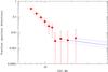 |
Fig. 13 Fraction of spurious X-ray detections as a function of detection likelihood for exposure times greater than 4000 s. The differential fraction of spurious detections in the lowest bin decreases to about 30 per cent. This plot has to be compared with the lower panel of Fig. 12, which shows the fraction of spurious sources for the whole sky (excluding fields that have been masked). |
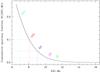 |
Fig. 14 Cumulative fraction of spurious detections as a function of detection likelihood. The dashed lines indicate the corresponding values for 20, 10, 5, 2, and 1 per cent (from top left to bottom right), see text for details. |
4.4.2. Sources only present in either 1RXS or 2RXS
Unfortunately, the 1RXS source detection software is not operational anymore and a direct comparison of the number of spurious detections cannot be made using simulations. To quantify which catalogue is more reliable, we have made correlations with other X-ray catalogues for those survey sources that are included in either the 1RXS or the 2RXS catalogue for detection likelihoods between 7.5 and 14.5. (in 1RXS the lowest likelihood bin is strongly incomplete because of the additional constraint of counts≥ 6). A search radius of 60 arcsec was applied for the 2RXP and the XMMSL1 catalogues. Because of the better spatial resolution, a search radius of 30 arcsec was used for the 3XMM and the 1SXPS catalogues.
For sources unique to 2RXS, we find 523 2RXP matches, while for sources unique to 1RXS the number of matches is lower with 394, which is about a factor of 1.4 in the percentages. The same holds for the correlations with the slew survey XMMSL1, where 136 1RXS and 211 2RXS counterparts are found, which is about a factor of 1.6 in percentages. For the 3XMM catalogue we find similar numbers in the fractions of associations, while for the 1SXPS catalogue a higher fraction of 2RXS counterparts with a factor of 1.16 is found. We speculate that the 3XMM catalogue might be also affected by a high number of spurious detections at the faint end, which appears not be the case of the other catalogues (see Table 2). In summary, the fraction of unique 2RXS sources (i.e. not contained in 1RXS) with counterparts in other X-ray catalogues is higher at the faint end than there are 1RXS sources without 2RXS counterparts (except 3XMM). This indicates that the 2RXS catalogue is more reliable in terms of spurious source content than 1RXS.
Although at the faint end the 2RXS catalogue contains a substantial number of spurious sources (as expected from low likelihood values), the contamination in the 2RXS catalogue is a lower limit for the 1RXS catalogue.
Cross-correlations for 1RXS and (clean) 2RXS catalogue sources with EXI_ML in the range 7.5−14.5.
4.5. Positional offset in scan direction
4.5.1. RASS-2 versus RASS-3 processing
We found a systematic positional offset in ecliptic coordinates between the 1RXS catalogue (RASS-2 processing) and detections based on event files from the RASS-3 processing. This shift is preferentially along ecliptic great circles (i.e. scan direction). An important parameter influencing the astrometry of the ROSAT sources is a time delay between the star tracker time and the photon arrival times. This time delay was determined for the RASS-2 processing to 2.53 s. After the RASS-2 processing, a rounding error was found in the software and corrected for the RASS-3 processing, but without re-adjusting the time delay. While in the RASS-2 processing the rounding error was largely compensated for by the time delay, a systematic coordinate shift along the scan direction was introduced in the RASS-3 processing that is present in the public event files. Because the scan direction reversed several times during the survey, the coordinate shift changes sign at scan reversals.
In Fig. 15 a histogram of the average position offsets in ecliptic latitude, that is, in scan direction, as a function of ecliptic longitude (progressing survey) is presented. At the scan reversals, the offsets change sign. Offsets between RASS-2 and RASS-3 in the ranges [−1, −5]′′ and [+1, +5]′′ are indicated with blue and red, respectively, showing the clear split depending on scan direction. In the following we refer to the longitude ranges (equivalent to time ranges of the six-month survey phase) with offset shifts preferentially negative and positive as blue and red periods.
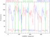 |
Fig. 15 Histogram of the positional offsets in ecliptic latitude between the 1RXS and 2RXS catalogues as a function of ecliptic longitude (LAMBDA). The blue lines indicate distance differences between −1″ and −5″, the red lines refer to differences between + 1″ and + 5″. The green vertical lines indicate the scan reversals. |
In Fig. 16 we show the positional offsets in ecliptic coordinates for RASS-3 detections that have 1RXS counterparts. For the blue periods of Fig. 15 the mean positional offset in ecliptic latitude β is Δβ = −3.110″ and the mean positional offset in ecliptic longitude λ is Δλ = + 0.031″. For the red periods the corresponding offsets are Δβ = + 3.134″ and Δλ = + 0.031″. The positional offset is dominant in scan direction β.
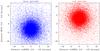 |
Fig. 16 Offsets in ecliptic coordinates between RASS-2 (1RXS) and RASS-3 positions, that is, before corrections applied for 2RXS. Depending on scan direction, a shift in scan direction of about + 3.1″ or −3.1″ is seen. For more details see Sect. 4.5.1. |
This systematic positional offset can be corrected for each photon of which the scan direction is known. The values determined above adjust the positions from RASS-2 and RASS-3 processing. Comparison of the coordinates with optical catalogues shows that an additional correction is required to minimise positional offsets in ecliptic latitude. As an intermediate step, we therefore corrected the missing time delay adjustment by applying a ± 3.14′′ positional shift in ecliptic latitude depending on the scan direction (and scan reversals) in our RASS-3 processing as a first iteration and used the new positions for comparison with optical catalogues (see next subsection).
In Fig. 17 we show an example for the scan rate (black line) determined from the attitude data that is available in 1 s steps, in units of arcsec s-1, before and after a scan reversal. The red dashed lines indicate at which times the ROSAT PSPC detector was switched on and good time intervals have been identified. For these periods photons are available for correction.
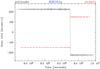 |
Fig. 17 Example for the speed of the ROSAT all-sky survey scanning as a function of time before and after a scan reversal. The alternating spreads correspond to a positional offset in scan direction of + 3.14″ and −3.14″ or a time delay between the photons in the RASS-2 and RASS-3 processing of 14.3 ms. The dashed red lines indicate time intervals when photons have been collected. |
In Fig. 18 we present the positional offset in ecliptic coordinates after applying a shift of ± 3.14′′ in ecliptic latitude to each RASS-3 event depending on scan direction. The systematic offset in ecliptic latitude present in Fig. 16 is now reduced to sub-arcsec level. For the blue periods of Fig. 18 the remaining mean positional offset in ecliptic latitude is Δβ = −0.308′′ and in ecliptic longitude Δλ = 0.039′′. For the red periods the positional offsets are Δβ = + 0.314′′ and Δλ = + 0.052′′.
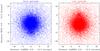 |
Fig. 18 Same as Fig. 16 after applying a ± 3.14″ shift in ecliptic latitude to the events of RASS-3 processing. The systematic offset in scan direction has been reduced by a factor of about 10, and the positional offsets in ecliptic coordinates are in the sub-arcsec range. |
Shift and separation of RASS X-ray and optical positions (from RBS and SDSS cross-correlation catalogues) in ecliptic latitude β in arcsec depending on ecliptic longitude (i.e. scan direction).
The absolute astrometry is described in the following section. Section 4.5.3 describes the correlation between the Tycho-2 catalogue and 2RXS, which gives an additional indication that 2RXS is more reliable.
4.5.2. Absolute astrometry
The absolute astrometry of the RASS-3 (after the 3.14′′ correction) and RASS-2 positions can best be tested with catalogues of point-like ROSAT sources that have been identified optically and whose optical positions have been accurately determined. Such catalogues are the ROSAT Bright Survey (RBS) catalogue from Schwope et al. (2000), and the SDSS catalogue of stars detected in the RASS (Agüeros et al. 2009). We have selected entries from the two catalogues that possess optical identifications for ROSAT sources with optical positional errors smaller than 1′′. For RBS we restricted ourselves to point-like entries of the classes AGN, star, cataclysmic variable, and X-ray binary, and did not consider extended emitters such as clusters or groups of galaxies, for which the extent increases the intrinsic X-ray positional uncertainty.
The correlation results with the RBS and SDSS catalogues are summarised in Table 3. The positional offsets for RASS-2 (1RXS) and RASS-3 still show a split depending on scan direction, indicating that there is a remaining component related to an uncorrected time delay shift. As this time delay was only given with two decimals for 1RXS, this corresponds to an uncertainty of ± 5 ms (~ ± 1′′). Therefore, a further shift in β beyond the pure rounding error adjustment is justified, and we applied a final ± 3.70′′ shift depending on scan direction. A 3.70′′ positional offset in scan direction corresponds to a star tracker time delay of 2.532 s (using the satellite rotation period of 96 min to scan a full great circle) compared to the previously implemented 2.53 s. The final offset histograms for point-like RBS sources and X-ray stars in SDSS are shown in Figs. 19 and 20, respectively.
For the 2RXS catalogue production we have shifted the sky positions for each individual event in ecliptic latitude (scan direction) and created new photon event tables. We repeated the source detection procedure with the same parameters as for the original RASS-3 processing. We made the new event tables publicly available and refer to the final corrected files as RASS-3.1 photon event tables.
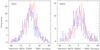 |
Fig. 19 Positional offsets in ecliptic latitude between the 1RXS catalogue and the optical positions from the Schwope et al. (2000) catalogue for red and blue periods (left panel), and similarly with respect to the 2RXS catalogue (right panel). |
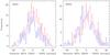 |
Fig. 20 Positional offsets in ecliptic latitude between the 1RXS catalogue and the optical positions from SDSS data (Agüeros et al. 2009) for red and blue periods (left panel), and similarly with respect to the 2RXS catalogue (right panel). |
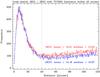 |
Fig. 21 Distribution of the angular separation of 1RXS (red) and 2RXS (blue) sources from nearest Tycho-2 catalogue entries. Statistical values for mean and median are computed below 40 arcsec (chance coincidences start to dominate above 40 arcsec, but have not been subtracted here). No selection on Tycho-2 positional errors has been performed in this plot. |
 |
Fig. 22 NEP analysis by Henry et al. (2006) compared to the 2RXS sources for field 930 521. Shown are the broad- (channels 11−235), soft- (11−41), and hard- (52−201) band images from top to bottom. All sources from the catalogue of Henry et al. (2006) are marked with blue circles and are also detected in our analysis (green squares). |
4.5.3. Correlation with Tycho-2
The ROSAT survey sources were correlated with the stellar Tycho-2 catalogue (Høg et al. 1998) to compare absolute positional accuracies of 1RXS and 2RXS detections. In Fig. 21 we show the distributions of angular separations for 1RXS (red) and 2RXS (blue). The significantly higher tail of 1RXS with respect to 2RXS might be interpreted as more spurious sources and/or greater positional errors for sources with larger separations for Tycho-2 counterparts. For distances ≤ 40 arcsec, the mean and median values for 1RXS and 2RXS are comparable (mean 15.6 and 15.2, median 13.3 and 12.9, respectively), with 2RXS values being slightly more accurate.
5. Comparison with other source detections in deep ROSAT exposure regions
The comparison of different source detection algorithms is of importance to evaluate the quality of the 2RXS source detections, especially in the Ecliptic Pole regions, which have the deepest exposures of the entire ROSAT all-sky survey. Henry et al. (2006) performed such an analysis and produced the deepest large solid-angle contiguous sample of 442 X-ray sources in a 80.6 deg2 region around the North Ecliptic Pole (NEP). In Fig. 22 we compare the sources detected in the NEP region by Henry et al. (2006) with our 2RXS sources. The figure shows, from top to bottom, the images of broad, soft, and hard energy bands (see Sect. A.2 for the definition of the energy bands). We use these three energies in the selected images because this lets us evaluate better the detection of soft and hard 2RXS sources. All sources from the analysis of Henry et al. (2006) are also detected as 2RXS sources. As the 2RXS detection limit extends down to an existence likelihood value of 6.5 (in contrast to the limit of 10 used by Henry et al. 2006), we find additional, weaker sources, which are shown as green squares.
6. Cross-matches of the 2RXS sources
We performed spatial cross-correlations with various other catalogues. Using simply the nearest neighbour to the X-ray position within 1′ , we point out that these cross-correlations do not always provide the most likely identification of the X-ray source, but reveal only potential counterparts. For the cross-correlations we included the following X-ray source catalogues: 1RXS (Voges et al. 1999), 2RXP (ROSAT Collaboration 2000), 3XMM (Rosen et al. 2016), XMMSL1 (Saxton et al. 2008), 1SXPS (Evans et al. 2014), and object lists for active galactic nuclei (Véron-Cetty & Véron 2010), for stars (Tycho2, Høg et al. 2000), the bright star catalogue (BSC, Ochsenbein & Halbwachs 1999), a catalogue of low- and high-mass X-ray binaries (Liu et al. 2001), a catalogue of high-mass X-ray binaries (Liu et al. 2006), a pulsar catalogue (Hobbs et al. 2004), and the catalogue of variable 1RXS sources (Fuhrmeister & Schmitt 2003). The nearest counterpart in the cross-matching catalogues to a 2RXS source is listed in our catalogue. A more detailed and sophisticated source identification work is beyond the scope of this paper and will be presented in a paper by Salvato et al. (in prep.).
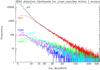 |
Fig. 23 2RXS detection likelihood distributions for all detections (black) and for purely spatial cross-matches within 60 arcsec with the X-ray catalogues 1RXS (red), 2RXP (cyan), 3XMM_dr4 (blue), XMMSL1_dr6 (green), and 1SXPS (magenta), with a bin size of 0.25 of EXI_ML. |
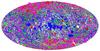 |
Fig. 24 Aitoff projection in Galactic coordinates of the sky distribution of 2RXS sources with HR1 errors smaller than 0.5. The size of the data points scales with the source count rate, and the colour represents the HR1 value. Sources in the hardness ratio intervals HR1 = [−1.0,−0.5] are indicated in red, HR1 = [−0.5,0.0] in magenta, HR1 = [0.0, + 0.5] in green, and HR1 = [ + 0.5, + 1.0] in blue. |
In Fig. 23 we illustrate the performed cross-matches with the catalogues listed above as a function of the 2RXS detection likelihood. At high 2RXS detection likelihoods these (usually bright) sources should almost always be detected in other X-ray catalogues, if they have been spatially covered (unless they show strong variability or an extremely different spectrum). The XMM slew survey catalogue XMMSL1 has the highest matching fraction at high EXI_ML values because it has the highest spatial coverage. At low EXI_ML values the sensitivity of XMMSL1 is generally too low to detect many of the 2RXS sources, and the matching fraction curve flattens. The 3XMM catalogue has the smallest spatial coverage but is also deepest, and therefore the curve is steepest. The comparison with the 1RXS catalogue shows that it becomes incomplete toward the faint end with respect to 2RXS. This is explained in Sect. 4.2 and is related to the width of the EXI_ML distribution.
7. 2RXS catalogue properties
7.1. Sky distribution in count rate and hardness ratio
The sky distribution of the 2RXS sources is shown in Fig. 24. The size of the symbols scales with count rate4, covering values between 0.001 and 68 counts s-1, while the colours represent different hardness ratio ranges (for the definition of hardness ratios see Appendix A.2). Red sources indicate soft and super-soft sources, often characterised with steep X-ray photon indices, while blue sources mark hard sources, typically with flat X-ray photon indices. We only show the 88 586 objects whose errors on the hardness ratio 1 (HR1) are smaller than 0.5. The faintest sources are detected in the North and South Ecliptic Pole regions, where the exposure time is longest.
7.2. General properties
In this section we discuss the distributions of the source count rates, the source counts, the existence likelihood, and the exposure time of the 135 118 2RXS sources. The distributions of existence likelihoods, count rates, and the source counts are given in Fig. 8. The distribution of source counts ranges between 3 and 35 033 counts. The distribution of the existence likelihood ranges between 6.5 and 26 198. Exposure times range between 7 s and 39 214 s.
7.3. Timing properties
In this section we compare the count rates of the 2RXS sources with those from ROSAT pointed observations, the XMM-Newton slew survey, and the 3XMM source catalogue. Additionally, we discuss the 2RXS source variability during the survey scans. We list the sources with most interesting timing properties based on our light curve analysis. A complete and detailed analysis is beyond the scope of this paper.
7.3.1. 2RXS versus ROSAT pointed observations
In Fig. 25 we compare the mean count rates of sources both detected in 2RXS and in ROSAT PSPC pointed observations (2RXP). This plot illustrates the degree of variability between the ROSAT survey and pointed observations. Count rate variations by more than a factor of 100 are found. We list the sources whose count rate variations between survey and pointed observations exceed a factor of 50 in Table B.1. This is expected because of the longer exposures and therefore higher sensitivity of the pointed observations. This is also seen in Fig. 25, where lower count rates are reached in the pointed observations.
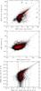 |
Fig. 25 Count rates of ROSAT 2RXS sources versus count rates derived from 2RXP ROSAT pointed observations (top), XMM-Newton slew survey count rates (middle), and 3XMM fluxes (bottom). For the assumed power-law model and derived conversion factors see text. |
7.3.2. 2RXS versus XMM-Newton slew survey
Here we compare the 2RXS count rates with count rates of XMM-Newton slew survey counterparts (XMMSL1). Although the XMM-Newton slew survey and the ROSAT survey observations have similar overall sensitivities in the 0.5−2 keV energy range (Saxton et al. 2008), the energy dependence of the effective areas is different between ROSAT and the EPIC-pn instrument of XMM-Newton. Assuming a power-law spectral model with photon index 1.7 and observed X-ray absorption of 3 × 1020 cm-2 (Watson et al. 2009), a factor of 8.38 higher count rate is expected for EPIC-pn. We have therefore used the XMM-Newton slew conversion factor of 8.38 to convert 2RXS count rates into 2RXS scaled count rates. We compare the 2RXS scaled count rates with count rates for the XMM-Newton slew survey objects (EPIC-pn, medium filter, 0.2−2 keV band) in Fig. 25. Outliers in Fig. 25, far away from this relation, are candidates for high variability. The deviation from the one-to-one line arises because XMMSL1 has a lower sensitivity than 2RXS, which is of the order of about one counts s-1, while the 2RXS count rates decrease to about a few 10-3 counts s-1. This is also obvious from Fig. 23, where the XMMSL1 is shown with the green line, becoming incomplete at low detection likelihood values.
7.3.3. 2RXS count rates versus 3XMM fluxes
To convert 2RXS count rates into fluxes (assuming the power-law model), a factor of 1.08×10⁻¹¹ erg cm-2 needs to be applied. In addition to the different effective areas, the flux limits are very different for 2RXS sources and the deeper 3XMM pointed observations. The 2RXS flux limit is about 10-13 erg cm-2 s-1, indicated by the vertical line in Fig. 25, while the 3XMM flux limit is much deeper with about 10-16 erg cm-2 s-1. Most of the faint 3XMM sources near the ROSAT flux limit have no real counterparts in the 2RXS catalogue and are spurious chance associations. This is shown in Fig. 25, where the correlation is clearly no longer linear near the ROSAT flux limit. Most of the 3XMM counterparts have fainter fluxes (below the one-to-one line) because the 3XMM count rate limit is lower than that of 2RXS.
7.3.4. Source variability during ROSAT survey scans
To characterise the temporal behaviour of the 2RXS sources, we have calculated the normalised excess variance with its uncertainty and the maximum amplitude variability during the survey scans. The light curves were background subtracted as described in Sect. 2.2.3. We automatically searched for cases where the net count rate decreases for up to three data points to low values, mostly below ~ 1 countss-1, caused by an increase in the background count rate. Most likely, events of strong solar activity or an increased particle background are responsible for this. Because the extraction for source and background events is not simultaneous (Sect. 2.2.3), short background flares are not always subtracted properly.
The normalised excess variance is a powerful and commonly used method to determine the probability that a time series shows variability above a certain threshold (e.g. Nandra et al. 1997; Vaughan et al. 2003; Ponti et al. 2004). For the 2RXS sources we have calculated the normalised excess variance with the formula ![Mathematical equation: \begin{eqnarray} \sigma^2_{\rm rms} = \frac{1}{N \mu^2} \sum_{i=1}^N\left[\left(X_i - \mu\right)^2 - \sigma^2_i\right] \end{eqnarray}](/articles/aa/full_html/2016/04/aa25648-15/aa25648-15-eq100.png) (1)and the uncertainty
(1)and the uncertainty 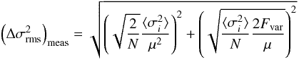 (2)where Fvar = σrms/μ is the fractional variability, N is the number of time bins, μ is the weighted (by exposure time) mean of the count rates, Xi and σi are the count rates and the corresponding uncertainties. The weighted mean was used because during the survey scans some time intervals exhibit low exposure times (of about 10 s) that are due to periods of high background, resulting in large errors bars in the data points in the survey light curves. With the unweighted mean the calculation of the mean count rate would result in incorrect values for the mean count rate. In combination with the uncertainty of the normalised excess variance, the ratio of both quantities gives the probability that a 2RXS source is time variable in units of Gaussian σ. For 0.9 per cent of the objects we find extremely short exposure times (shorter than or equal to 6 s) for the data points in the survey light curve. We have flagged these light curves and objects.
Fuhrmeister & Schmitt (2003) have performed a systematic study of X-ray variability in the ROSAT all-sky survey for 1RXS sources in the BSC and FSC with an existence likelihood greater than or equal to 15. 2RXS sources with X-ray variability significance values above 10σ, but not listed Fuhrmeister & Schmitt (2003), are given in Table B.2. 2RXS sources with significance values above 20σ are listed in Table B.3. These sources are listed in Fuhrmeister & Schmitt (2003), but they are not shown as graphical representations. An example is shown in Fig. 27.
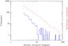 |
Fig. 26 Histogram of sources with excess variance values above 3σ. The differential distribution is shown as the blue histogram. The solid red-dashed lines delineate the integral distribution. |
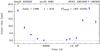 |
Fig. 27 Example for a source with excess variance above the 3σ limit. The source is known as VV Pup, an AM CV with an orbital period of about 100 min. As the ROSAT light curve samples close to the intrinsic period, we see an aliasing effect caused by the convolution of the true variation and the window function. |
In addition to the normalised excess variance, which describes the variability of a survey light curve as a whole, we calculated the maximum amplitude variability to search for flaring events during the survey observations. To calculate the maximum amplitude variability ampl_max and its significance ampl_sig, we used the maximum count rate cmax, the corresponding error cmax_err, the minimum count rate cmin, and its corresponding error cmin_err for each survey light curve. The maximum amplitude variation and its significance is then 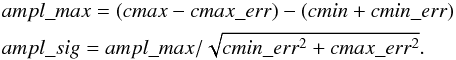 In Table B.4 we list objects with significance for the maximum amplitude variability above 10σ. Figure 28 shows the distribution of sources with maximum amplitude variability above the 3σ limit. An example is shown in Fig. 29.
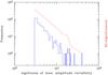 |
Fig. 28 Distribution of the significance values of the maximum amplitude variability for 2RXS above the 3σ limit. The differential distribution is shown as the blue histogram. The solid red-dashed line delineates the integral distribution. |
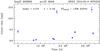 |
Fig. 29 Example for a source passing the maximum amplitude variability test. |
A variability test was applied to the 3XMM catalogue by the authors using a χ2 test. Sources with a probability lower than 10-5 of being constant were flagged as variable sources. About 30 000 of the 151 524 1SXPS sources are classified as variable sources.
7.4. Spectral analysis
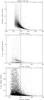 |
Fig. 30 Distribution of the source counts in relation to the error of the photon index, the temperature error derived from the mekal, and the temperature error from the black-body fits (from top to bottom). For all three spectral models the errors for fewer than 100 source counts are broadly distributed. Therefore, we applied a limit of at least 100 source counts for the spectral fit results presented here. |
We have performed spectral fits using three different models: (i) a power law (powl); (ii) an optically thin plasma emission model (mekal); and (iii) an optically thick black-body model (bbdy). Spectral fitting was performed in EXSAS (Zimmermann et al. 1998). Absorption by neutral gas with solar elemental abundances (Morrison & McCammon 1983) was included for all models. From the fits, we stored the absorbing hydrogen column density (NH), powl photon index, mekal, and bbdy temperatures and model normalisations together with the corresponding errors, reduced  value, χ2 value, the number of data points used in the fit, and the number of degrees of freedom. The absorption-corrected flux was calculated for all spectral models. We note that the (absorption-corrected) fluxes for a given source for the different models can be very different when the NH values differ strongly. For comparison with the NH values derived from the spectral fits, we determined the Galactic absorption in the direction of each source NH, gal following Dickey & Lockman (1990).
To include only spectral parameters in the catalogue that result from acceptable fits, we only accepted spectral fits with a reduced χ2 lower than 1.5 and with at least four degrees of freedom.
In Fig. 30 we show the errors of the principal model parameters – photon index, plasma temperature and black-body temperature – as a function of the number of source counts. In all three plots we find that the parameter errors strongly increase for spectra with fewer than 100 source counts. Therefore, we applied an additional cut to require at least 100 source counts in the spectrum. We note that in all three plots in Fig. 30 there are still sources with large parameter errors, even for large numbers of source counts. We inspected these spectra and found that they are mainly from highly absorbed sources, with NH values close to or even above 1022 cm-2. In such cases the photon indices and the temperatures can only be poorly constrained in the available narrow energy band. However, the information on the NH value is important, which is the reason for providing these fit parameters. The number of sources that fulfil the criteria on reduced χ2, number of degrees of freedom (which is practically fulfilled for sources with more than 100 counts), and the minimum number of source counts are 2722, 455, and 1769 for the power law, the mekal, and the black-body fits, respectively. For the mekal and black-body fits we furthermore required that the error of the temperatures is smaller than one-third of the temperature values. For the power-law fit the limit on source counts is sufficient to constrain the photon indices with adequate precision.
7.4.1. Power-law model
The parameters obtained from a simple power-law fit are the photon index Γ, the normalisation parameter, the NH, and their corresponding errors. From the spectral fits we calculated the absorption-corrected flux. Figure 34 (upper panel) shows an example for a spectral fit with a simple power-law model for the 2RXS source 931037_0107 (Mrk 501). In Fig. 31 we show the distribution of the photon indices. The histogram peaks at around 2, decreasing towards lower and higher photon indices.
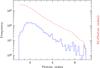 |
Fig. 31 Histogram (blue) of the distribution of photon indices between 1 and 7 for sources with at least 100 source counts, at least four degrees of freedom and reduced χ2 values lower than 1.5. The red dashed line gives the integral distribution. |
7.4.2. Plasma-emission model
In addition to the power-law fit, we have performed spectral fits for optically thin plasma emission using the mekal model. The parameters obtained from these fits are the plasma temperature, the normalisation, and the NH value. Figure 34 (middle panel) gives an example of a spectral fit with the mekal model.
In Fig. 32 we show the distribution of the temperatures obtained from the mekal fit of Mewe et al. (1985) and a temperature error smaller than one-third of the best-fit temperature. A bimodal distribution is clearly visible in the temperature, with one peak at around 0.2 keV, and the second peak centred on around 0.7 keV. We note that the 0.2 keV peak might be slightly affected by the C-Kα absorption edge, which may not be adequately accounted for by the instrumental corrections, therefore not all of these objects may have the correct mekal temperature. This was pointed out by Prieto et al. (1996). The second peak at around 0.7 keV is also found in XMM-Newton data for optically thin diffuse emission in NGC 6240, for instance (Boller et al. 2003). Similar plasma temperatures have been found in nearby galaxies.
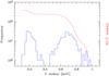 |
Fig. 32 Distribution of the temperatures obtained from the fits using the mekal model for sources with at least 100 source counts, reduced χ2 values lower than 1.5, at least four degrees of freedom and temperature error smaller than one-third of the best-fit value. The differential distribution is shown as the blue histogram. The red dashed line gives the integral distribution. |
7.4.3. Black-body model
As a third spectral model we have applied black-body fits with neutral foreground absorption to the 2RXS sources. The parameters obtained from these fits are the black-body temperature, the normalisation, and the NH value. Figure 34 (lower panel) gives an example for a spectral fit with a black-body model.
In Fig. 33 we show the distribution of the temperatures obtained from the black-body fit, again for sources fulfilling the criteria described by the mekal model. As for the mekal model, a bimodal distribution in the temperature is found with one peak at around 0.2 keV, similar to the peak found for the mekal fits, and the second peak centred on around 20−30 eV (containing 11 sources). Nine of these latter sources are optically identified white dwarfs, and the other two are AM-Her type cataclysmic variables. These nine are also listed in Fleming et al. (1996) as White Dwarfs. All 11 objects are detected with the ROSAT Wide Field Camera (Pye et al. 1995), which is sensitive in the extreme soft band from 60 to 200 eV.
The lower peak is a factor of 10 lower than the 0.2 keV peak in the mekal fits, indicating that black-body fits yield better results for objects with lower temperatures. This is most probably due to the fitting of different physical emission mechanism, for instance, optically thin gas with the mekal fits, and optically thick black-body emission from accreting objects.
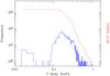 |
Fig. 33 Same as Fig. 32 for the black-body model. The differential distribution is shown as the blue histogram. The solid red dashed lines delineates the integral distribution. |
7.4.4. Constraints from spectral fits
As a result of the rather narrow spectral band-path of ROSAT – between the low-energy cutoff by interstellar absorption and the high-energy cutoff by the mirror – and the limited spectral resolution (E/ΔE ~ 4), the significance of the spectral fits depends on the number of counts and on the column density. Of the 2722 spectra with an acceptable fit quality for the power-law model, 1769 and 455 spectra also yield acceptable fits for the black-body and mekal model, respectively. For 247 sources all three spectral models give an acceptable fit (for an illustration see the top panel of Fig. 35).
However, the following question is far more interesting than the statistics of overlaps: How many sources with more than 100 counts can be fitted with only one of the spectral models with χ2 lower than 1.5? The answers are 1117, 119, and 79 for the power-law, black-body, and mekal fits, respectively. The lower panel of Fig. 35 shows that the number distributions for sources with a unique acceptable spectral fit are not significantly different, which indicates that the uniqueness of the acceptable spectral model does not depend on the photon statistics.
An example for an acceptable power-law fit to Mrk 421 and for the unacceptable mekal and black-body fits is given in Fig. 34. For each fit three panels are presented, showing (1) the PSPC spectrum (data points with errors) together with the best-fit model as a solid line; (2) the unfolded spectrum with the model; and (3) the residuals. Best-fit model parameters are listed.
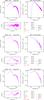 |
Fig. 34 Example of individual 2RXS source-level product: power-law, mekal, and black-body fit to Mrk 421 (from top to bottom). The reduced χ2 values are 1.1, 10.0, and 5.0 for the power-law, mekal, and black body fits, respectively. |
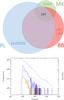 |
Fig. 35 Top panel: graphical illustration of the number of acceptable spectral fits for the three models. The size of the circles scales with the number of spectra with acceptable fits. The number of sources with acceptable power-law, mekal, and black-body fits are 2722, 455, and 1769, respectively, while 1117, 79 and 119 sources have an acceptable (unique) fit with only one of the models. For more information see Sect. 7.4.4. Bottom panel: differential and integral distributions for sources with unique power-law, black-body, and mekal fits in blue, red, and green, respectively. |
7.4.5. Flux distributions
Additionally, we have calculated absorbed fluxes for the sources selected in the previous subsections for spectral fitting. This is important for two reasons: (i) some sources are highly absorbed, and only photons above 1.5 keV are detected. The extrapolation to an intrinsic unabsorbed flux becomes highly uncertain and unphysical. (ii) Absorbed fluxes can be related to count rates by an energy-conversion factor. For the power-law, the mekal, and the black-body models, the absorbed fluxes with unique spectral fits range between 1.0 × 10⁻⁹ and 8.8 × 10⁻¹⁴, 1.0 × 10⁻¹⁰ and 1.7 × 10⁻¹³ and 9.8 × 10⁻¹⁰ and 1.4 × 10⁻¹³ erg cm-2 s-1, respectively. For all three spectral models we find a similar lower flux limit of the 2RXS sources of a few times of 10-13 erg cm-2 s-1.
8. 2RXS web page, catalogue interface, and help desk
A description of the catalogue is available on the catalogue web site. There, we also provide an interface to access the 2RXS catalogue and related products. The basic X-ray properties, correlations with sources from other X-ray missions and cross-matches as described in Sect. 6, an X-ray image, the X-ray light curve, and the spectral properties (for sources fulfilling the criteria described in Sect. 7.4) are available for each 2RXS source. A complete description of the catalogue entries is available at the catalogue web site. In addition, we present X-ray images where markings are applied to the source and background extraction regions. These were used to produce background-subtracted light curves and spectra. A cone search has been implemented, available at the catalogue web site, to efficiently access the 2RXS source properties and data products. Individual sources, the complete 2RXS catalogue, and corrected photon event files (RASS-3.1 processing) in FITS format can be accessed in the download area. We provide a 2RXS help desk for the community at the e-mail adress This email address is being protected from spambots. You need JavaScript enabled to view it. .
9. Summary
We have re-analysed the photon event files from the ROSAT all-sky survey. The main goal was to create a catalogue of point-like sources, which is referred to as the 2RXS source catalogue. We improved the reliability of detections by an advanced detection algorithm and a complete screening process. New data products were created to allow timing and spectral analysis. Photon event files with corrected astrometry and Moon rejection (RASS-3.1 processing) were made available in FITS format. The 2RXS catalogue will serve as the basic X-ray all-sky survey catalogue until eROSITA data become available.
In this paper we list the most interesting objects in terms of their timing and spectral properties. A discussion of the science highlights is beyond the scope of the paper. With the publication of the 2RXS catalogue and its data products, the detailed science specific exploration is now available for the astrophysical community.
The experience gained by the High-Energy Group at MPE in creating the new ROSAT all-sky survey X-ray source catalogue is being and will be fed into the data reduction analysis and scientific exploration of the forthcoming eROSITA all-sky survey.
This scheme has been kept also for the next RASS-3 processing.
Using the hyperbolic tangent function tanh(x) = (ex−e− x)/(ex + e− x).
ESO-MIDAS: http://www.eso.org/sci/software/esomidas/
For the EXSAS users guide and additional information for the used commands see web page (Sect. 8).
Using the command DETECT/LOCAL of the EXSAS package.
Produced with CREATE/SOURCE_DETECT_IMAGE
Due to restrictions in the EXSAS package the likelihood limits were increased by 5% until the number of detections per band and sub-image were less than 400.
CREATE/BG_IMAGE
DETECT/MAP
Due to restrictions in the EXSAS package the likelihood limits were increased by 5% until the number of detections per band and sub-image were less than 1000.
MERGE/SOURCE_LIST
DETECT/MAXLIK
Note that this ML algorithm can only return detections close to positions provided by the input lists. Therefore, care has to be taken that no proper source candidate is missed in previous detection steps.
Acknowledgments
We thank the anonymous referee for detailed comments, which improved this paper significantly. The authors thank Damien Coffey for critical reading of the manuscript, especially for improving the language. Jürgen Schmitt provided us unpublished light curves from their 1RXS source variability analysis. Joachim Paul performed detective work in our old archives for hints on attitude errors and has set up the 2RXS web page and catalogue interface. We appreciate discussions with Damien Coffey and Mara Salvato on positional offsets and source identification procedures. This research has made extensive use of the SIMBAD database and of the VizieR catalogue access tool, both operated at CDS, Strasbourg, France (see descriptions in Wenger et al. 2000 and Ochsenbein et al. 2000). This work would have been impossible without the old ROSAT staff (H/W + S/W), who are too numerous to mention individually.
References
- Agüeros, M. A., Anderson, S. F., Covey, K. R., et al. 2009, ApJS, 181, 444 [NASA ADS] [CrossRef] [Google Scholar]
- Aschenbach, B. 1988, Appl. Opt., 27, 1404 [NASA ADS] [CrossRef] [Google Scholar]
- Banse, K., Grosbol, P., & Baade, D. 1992, in Astronomical Data Analysis Software and Systems I, eds. D. M. Worrall, C. Biemesderfer, & J. Barnes, ASP Conf. Ser., 25, 120 [Google Scholar]
- Boese, F. G. 2000, A&AS, 141, 507 [NASA ADS] [CrossRef] [EDP Sciences] [Google Scholar]
- Boese, F. G. 2004, A&A, 426, 1119 [NASA ADS] [CrossRef] [EDP Sciences] [Google Scholar]
- Boese, F. G., & Doebereiner, S. 2001, A&A, 370, 649 [NASA ADS] [CrossRef] [EDP Sciences] [Google Scholar]
- Boller, T., Keil, R., Hasinger, G., et al. 2003, A&A, 411, 63 [NASA ADS] [CrossRef] [EDP Sciences] [Google Scholar]
- Dickey, J. M., & Lockman, F. J. 1990, ARA&A, 28, 215 [NASA ADS] [CrossRef] [MathSciNet] [Google Scholar]
- Evans, P. A., Osborne, J. P., Beardmore, A. P., et al. 2014, ApJS, 210, 8 [NASA ADS] [CrossRef] [Google Scholar]
- Fleming, T. A., Snowden, S. L., Pfeffermann, E., Briel, U., & Greiner, J. 1996, A&A, 316, 147 [NASA ADS] [Google Scholar]
- Forman, W., Jones, C., Cominsky, L., et al. 1978, ApJS, 38, 357 [NASA ADS] [CrossRef] [Google Scholar]
- Freyberg, M. J. 1994, Ph.D. Thesis, Ludwig-Maximilians-Univ. München [Google Scholar]
- Fuhrmeister, B., & Schmitt, J. H. M. M. 2003, A&A, 403, 247 [NASA ADS] [CrossRef] [EDP Sciences] [Google Scholar]
- Hasinger, G., Altieri, B., Arnaud, M., et al. 2001, A&A, 365, L45 [NASA ADS] [CrossRef] [EDP Sciences] [Google Scholar]
- Henry, J. P., Mullis, C. R., Voges, W., et al. 2006, ApJS, 162, 304 [NASA ADS] [CrossRef] [Google Scholar]
- Hobbs, G., Manchester, R., Teoh, A., & Hobbs, M. 2004, in Young Neutron Stars and Their Environments, eds. F. Camilo, & B. M. Gaensler, IAU Symp., 218, 139 [Google Scholar]
- Høg, E., Kuzmin, A., Bastian, U., et al. 1998, A&A, 335, L65 [NASA ADS] [Google Scholar]
- Høg, E., Fabricius, C., Makarov, V. V., et al. 2000, A&A, 355, L27 [NASA ADS] [Google Scholar]
- Liu, Q. Z., van Paradijs, J., & van den Heuvel, E. P. J. 2001, VizieR Online Data Catalog: V/106 [Google Scholar]
- Liu, Q. Z., van Paradijs, J., & van den Heuvel, E. P. J. 2006, A&A, 455, 1165 [NASA ADS] [CrossRef] [EDP Sciences] [Google Scholar]
- Mewe, R., Gronenschild, E. H. B. M., & van den Oord, G. H. J. 1985, A&AS, 62, 197 [NASA ADS] [Google Scholar]
- Morrison, R., & McCammon, D. 1983, ApJ, 270, 119 [NASA ADS] [CrossRef] [Google Scholar]
- Nandra, K., George, I. M., Mushotzky, R. F., Turner, T. J., & Yaqoob, T. 1997, ApJ, 476, 70 [NASA ADS] [CrossRef] [Google Scholar]
- Ochsenbein, F., & Halbwachs, J. L. 1999, VizieR Online Data Catalog: V/53A [Google Scholar]
- Ochsenbein, F., Bauer, P., & Marcout, J. 2000, A&AS, 143, 23 [NASA ADS] [CrossRef] [EDP Sciences] [Google Scholar]
- Pfeffermann, E., & Briel, U. G. 1986, in 597, X-ray instrumentation in astronomy, ed. J. L. Culhane, SPIE Conf. Ser., 208 [Google Scholar]
- Pfeffermann, E., Briel, U. G., & Freyberg, M. J. 2003, Nucl. Instrum. Methods Phys. Res. A, 515, 65 [Google Scholar]
- Ponti, G., Cappi, M., Dadina, M., & Malaguti, G. 2004, A&A, 417, 451 [NASA ADS] [CrossRef] [EDP Sciences] [Google Scholar]
- Prieto, M. A., Hasinger, G., & Snowden, S. L. 1996, A&AS, 120, 187 [NASA ADS] [CrossRef] [EDP Sciences] [Google Scholar]
- Pye, J. P., McGale, P. A., Allan, D. J., et al. 1995, MNRAS, 274, 1165 [NASA ADS] [Google Scholar]
- ROSAT Collaboration. 2000, VizieR Online Data Catalog: IX/30 [Google Scholar]
- Rosen, S. R., Webb, N. A., Watson, M. G., et al. 2016, A&A, in press DOI: 10.1051/0004-6361/201526416 [Google Scholar]
- Saxton, R. D., Read, A. M., Esquej, P., et al. 2008, A&A, 480, 611 [NASA ADS] [CrossRef] [EDP Sciences] [Google Scholar]
- Schwope, A., Hasinger, G., Lehmann, I., et al. 2000, Astron. Nachr., 321, 1 [NASA ADS] [CrossRef] [Google Scholar]
- Trümper, J. 1982, Adv. Space Res., 2, 241 [NASA ADS] [CrossRef] [Google Scholar]
- Trümper, J. 1993, Science, 260, 1769 [NASA ADS] [CrossRef] [PubMed] [Google Scholar]
- Vaughan, S., Edelson, R., Warwick, R. S., & Uttley, P. 2003, MNRAS, 345, 1271 [NASA ADS] [CrossRef] [Google Scholar]
- Véron-Cetty, M.-P., & Véron, P. 2010, A&A, 518, A10 [NASA ADS] [CrossRef] [EDP Sciences] [Google Scholar]
- Voges, W., Aschenbach, B., Boller, T., et al. 1996, IAU Circ., 6420, 2 [NASA ADS] [Google Scholar]
- Voges, W., Aschenbach, B., Boller, T., et al. 1999, A&A, 349, 389 [NASA ADS] [Google Scholar]
- Voges, W., Aschenbach, B., Boller, T., et al. 2000, IAU Circ., 7432, 3 [NASA ADS] [Google Scholar]
- Watson, M. G., Schröder, A. C., Fyfe, D., et al. 2009, A&A, 493, 339 [NASA ADS] [CrossRef] [EDP Sciences] [Google Scholar]
- Webb, N., & XMM-Newton Survey Science Centre 2014, in The X-ray Universe 2014, ed. J.-U. Ness, Online at http://xmm.esac.esa.int/external/xmm_science/workshops/2014symposium/, 331 [Google Scholar]
- Wenger, M., Ochsenbein, F., Egret, D., et al. 2000, A&AS, 143, 9 [NASA ADS] [CrossRef] [EDP Sciences] [Google Scholar]
- Wood, K. S., Meekins, J. F., Yentis, D. J., et al. 1984, ApJS, 56, 507 [NASA ADS] [CrossRef] [Google Scholar]
- Zimmermann, U., Boese, G., Becker, W., et al. 1998, Exsas Users Guide [Google Scholar]
Appendix A: Detection algorithm
Appendix A.1: Source detection algorithm
The source detection was performed using a three-step approach and is described in Sect. 2.1.
One goal of 2RXS is the detection of point-like sources down to a likelihood limit of 6.5; very extended sources are not dealt with here; the detailed discrimination is explained below in Sect. A.3. The detection algorithm follows the standard scheme that was applied for the BSC and FSC (Voges et al. 1999), with important extensions. The publicly available software packages ESO-MIDAS5 version P03SEPpl1.2 (Banse et al. 1992) and EXSAS6 version 05APR_EXP (Zimmermann et al. 1998) were used on a Linux platform throughout this analysis.
Appendix A.2: Energy bands
The PSPC response varies significantly over the bandpass of 0.1−2.4 keV, with a break at the carbon absorption edge (0.28 keV; cf. heasarc.gsfc.nasa.gov/docs/pspc_matrices.html). Several energy bands were constructed to determine the source properties. These are expressed in pulse-height-invariant channels in units of approximately 10 eV, broad (B): channels 11–235 (0.1–2.4 keV), soft (S): 11–41 (0.1−0.4 keV), hard (H): 52–201 (0.5–2.0 keV), as in Voges et al. (1999). In addition, we performed source detection in the following bands: medium (M): 52–90 (0.5–0.9 keV), very hard (V): 91–201 (0.9–2.0 keV), and wide (W): 11–201 (0.1–2.0 keV).
Source counts that were corrected for vignetting and dead-time were used to determine hardness ratios HR according to HR = (hard−soft)/(hard + soft) with the bands  (A.1)as in Voges et al. (1999).
Appendix A.3: Regions with very extended bright X-ray emission
The source detection algorithm is focused on point-like sources with an extent smaller than 5′ radius, therefore we excluded bright, extended emission features such as the Vela or Kepler supernova remnants. Thirty-two regions were manually identified and marked using polygon masks. Sources detected in these regions were later automatically flagged and excluded from the catalogue. In Table C.2 we list the sky fields that have been identified as such masked regions. These fields can be assessed through the the catalogue web page under cone search.
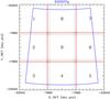 |
Fig. A.1 Sub-images used in our detection scheme: the whole frame corresponds to a full 6.4° × 6.4° RASS field, the blue area denotes the unique region (rectangle in equatorial coordinates, here for field 930507p). The red lines illustrate the unique areas for each sub-image, while the dashed lines show the overlap among the sub-images. All sub-images have the same size. sky_pix units are 0.5′′. The sub-image number USKY as well as the (X_SKY,Y_SKY) coordinate values for each detection are stored in the catalogue. For details see text. |
Sources with amplitude variability greater than 50 for sources included in both the survey 2RXS and pointed 2RXP catalogues.
Appendix A.4: Local detection
The first detection procedure is running a sliding window method7 on a binned image with 45′′ squared pixels8. Like in Voges et al. (1999), this is applied to an image with a size of 512 pixels × 512 pixels. One important extension that was added to the previous analysis by us is a multiple detection run on a mosaic of 3 × 3 overlapping sub-images of about 1/9 (12.6%) in area where the remainder is masked and thus not considered (see Fig. A.1). This leads to a total of ten detection lists per energy band and field, with a minimum existence likelihood of 5.5 for the sub-images and 6.0 for the full image9.
Appendix A.5: Creation of background map
Detection lists from the previous step with a minimum likelihood of 8.0 are used as input to excise the brightest sources with a cut radius of 5 FWHM of the PSF. A smoothed map is created when filling the holes with a 2d spline fit10. The multiple sub-image masking procedure is also applied to the background map creation process. Thus, bright sources or sharp emission gradients in one sub-image have no effects (over-shooting, etc.) on background maps of other sub-images.
Appendix A.6: Detection using background map
The sliding-window detection process is repeated using the smooth background maps 11 with a minimum existence likelihood of 5.5 for sub-regions, and 8.0 for the full image 12.
Appendix A.7: Source list merging (I)
The source lists produced by the local and map detection runs (three energy bands S, H, and B for each of the two runs) were merged 13 separately for each of the ten images for each of the 1378 fields. These lists were then used as input for the next step. The ten detection lists for each of the remaining three bands ( M, V, and W ) were kept for later individual inspection, but were not used explicitly in the catalogue production. Multi-band detection was performed sequentially and not simultaneously.
Appendix A.8: Maximum likelihood detection
After the image-based detection steps described above were completed, a photon-based algorithm ( Boese & Doebereiner 2001) was applied to use the full spatial resolution. The ten merged lists were used as input for a maximum likelihood evaluation of the candidate X-ray sources. Each photon is properly weighted for vignetting and detector dead-time, and the distribution is compared with a model of the PSF. Finally, the maximum likelihood algorithm 14 yields source positions and count rates for the broad energy band 15 . The final detection list was built from sub-image entries down to a detection limit of 5.5 and with full-field-only detections added above a limit of 7.0 (with a flag USKY==0 to recognise them).
Appendix A.9: Small-map source list merging (II)
After the source detection process, the detection lists were unified. First, the nine lists of the sub-regions were merged after limiting them to the unique areas in tangential plane-projected sky coordinates. Then, additional sources from full-field detection (if not already contained in the sub-image analysis) were included. Finally, detections were selected according to the rectangular equatorial coordinate ranges for each of the 1378 fields (see Fig. 2).
Appendix A.10: Automatic flagging and rejection
Detections inside masked regions were flagged and excluded from the catalogue. Of the close multiple (mostly pairs) detections (within 10 ′′ ), only the one with highest likelihood value was kept, while the others were flagged and excluded from the catalogue. Later, a visual screening was applied and further detections were flagged and removed (see Sect. 3).
Appendix A.11: Point spread function and detection cell size
The ROSAT PSPC survey point spread function (PSF) is almost energy independent in the range of 60%−90% encircled energy fraction (EEF, see Fig. 19 in Boese 2000), corresponding to an integration radius of 100−200 ′′ . The effective detection cell size of our multi-stage detection scheme has to be calibrated a posteriori using simulations (see also Sect. 5.7 in Zimmermann et al. 1998). In Fig. 12 we fit the likelihood function to the distribution of simulated spurious sources and derived an average number of detection cells per field of 11 000, corresponding to a detection cell size of 116 ′′ , equivalent to an EEF of 64.2%.
Appendix B: 2RXS sources with extreme variability
Appendix B.1: 2RXS sources versus ROSAT pointed observations
In Table B.1 we list 2RXS sources that were also detected in ROSAT pointed observations, which show amplitude variations greater than 50. Table B.1 also includes the count rates from 2RXS survey and 2RXP pointed observations, the source count ratio and the likely identification of the source.
Appendix B.2: Normalised excess variance.
In Table B.2 we list 2RXS sources that show normalised excess variance values above 10 σ , which are not listed in Fuhrmeister & Schmitt (2003 ) .
Sources with normalised excess variance values above 10σ and not listed in Fuhrmeister & Schmitt (2003).
Sources that posses normalised excess variance values greater than 20 σ and are listed in Fuhrmeister & Schmitt (2003 ) , but are not shown as graphical illustrations, are also listed in Table B.3 .
Sources with normalised excess variance values above 20σ and listed in Fuhrmeister & Schmitt (2003; FUH), but not shown as graphical illustration.
Appendix B.3: Maximum amplitude variability
In Table B.4 we list significant sources that have a maximum amplitude variability greater than 10 σ .
Sources with maximum amplitude variabilities above 10σ.
Appendix C: Extended X-ray emission regions with embedded point sources in the ROSAT all-sky survey
Sources added manually to 1RXS BSC, see text for details.
Large regions with extended X-ray emission in the ROSAT all-sky survey, masked in standard detection run.
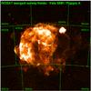 |
Fig. C.1 ROSAT all-sky image of the Vela SNR. In the upper right corner the SNR Puppis A is visible. We have merged the event files from several sky fields to produce the image. The size of the image is 10.5°× 10.5°. Details will be reported in a subsequent paper. |
For the 1RXS BSC catalogue, nine extended sources had been added manually as listed in Table C.1. No source detection
numbers, detection likelihoods, or (e.g.) count rates are available for them there. Six of them are very extended supernova remnants, which we have masked from our standard source detection procedure. Sco X-1 has never been observed with the ROSAT PSPC: during the survey, the PSPC had been switched off before scanning Sco X-1, and been switched on again afterwards. In the survey completion phase (Feb. 1997) most of this unobserved region has been filled up with pointed observations; also a lunar occultation observation of Sco X-1 had been performed (Feb. 1998). This will be described in Freyberg et al. (in prep.). The Vela SNR had been manually included in 1RXS with the coordinates of the Vela pulsar. We have detected the Vela pulsar automatically and included it in 2RXS (together with two other sources inside the Vela SNR region). The last entry in Table C.1 is due to single reflections from Nova Muscae in January 1991, and appeared as an extended emission region in the survey images. We did not add this to 2RXS.
We have identified 32 large extended regions with diffuse emission and embedded point sources, as well as large, brighter, and extended sources, such as clusters of galaxies or supernova remnants. These regions are listed in Table C.2 . For three of these extended regions the central source is included in the present 2RXS catalogue. We interactively determined the count rate of these regions and listed the source identification. The point source content of these regions will be published as additional survey sources in a separate paper (Freyberg et al., in prep.).
The mask in field 930738 corresponds to SNR G109.1-01.1 (CTB 109), with the central point source being 1E 2225.0+5837. For field 931232 the coordinates were obtained from the 2RXS processing for source 86 from central sub-image. In field 931316 two supernova remnants were detected, SNR G189.1+02.9 and SNR IC 433. Figure C.1 depicts the ROSAT all-sky survey image of the Vela SNR.
All Tables
Cross-correlations for 1RXS and (clean) 2RXS catalogue sources with EXI_ML in the range 7.5−14.5.
Shift and separation of RASS X-ray and optical positions (from RBS and SDSS cross-correlation catalogues) in ecliptic latitude β in arcsec depending on ecliptic longitude (i.e. scan direction).
Sources with amplitude variability greater than 50 for sources included in both the survey 2RXS and pointed 2RXP catalogues.
Sources with normalised excess variance values above 10σ and not listed in Fuhrmeister & Schmitt (2003).
Sources with normalised excess variance values above 20σ and listed in Fuhrmeister & Schmitt (2003; FUH), but not shown as graphical illustration.
Large regions with extended X-ray emission in the ROSAT all-sky survey, masked in standard detection run.
All Figures
|
Fig. 1 Structure and numbering scheme of the sky fields in the ROSAT all-sky survey in equatorial coordinates (courtesy K. Dennerl, available at the 2RXS web site.) Areas around the North and South ecliptic poles with 1° and 15° radius are indicated at the upper left and lower right corner. |
| In the text | |
|
Fig. 2 Example for a source count image of sky field 930304 in the way it is used for source detection. For the colour representation in this and all following images the ESO/MIDAS colour table heat is used with linear intensity scaling. The cyan solid lines confine the 6.4° × 6.4° field and the scan direction is marked with the yellow line through the centre of the field. 2RXS sources are indicated with green circles. Detections that were manually flagged as being uncertain (see Sect. 3) are marked with cyan crosses. Coordinates refer to the image centre, the exposure time is the median over the whole image. |
| In the text | |
|
Fig. 3 Example of X-ray count rate images for our six energy bands with overlaid X-ray intensity contours (black lines), bands 1 to 6 are defined as PSPC channels 11−41, 52−90, 91−201, 11−235, 52−201, 11−201, respectively (with one channel ~ 10 eV). Each image is centred on source 125 for which the 2RXS IAU name is provided. The broad-band source count rate (PSPC channels 11−235) with error as determined from the detection algorithm is in units of counts ks-1. Contour levels are in units of counts ks-1 arcmin-2. At the top of the image the field number (SeqID) and the source identification within the field (srcID) are given. The green circles gives the catalogue entries, and the cyan cross marks a source that was visually flagged in the screening process. |
| In the text | |
|
Fig. 4 X-ray light curve of 2RXS J043339.0+741012. The mean count rate, the corresponding standard deviation (both in counts s-1), and the normalised excess variance with 1σ uncertainty are given. |
| In the text | |
|
Fig. 5 Example of a control image demonstrating how the background region is selected. The background regions for source 27 are shown in cyan (at the top) and yellow circles (at the bottom). Since the yellow circle is contaminated with another source (33), the background in the cyan circle is used in the background subtraction. |
| In the text | |
|
Fig. 6 Top: example of a source that is considered as a correct detection, i.e. the source flag is set to zero. The broad-band image is shown. The object is identified as white dwarf WD 1501+663. Bottom: example of an uncertain detection (number 167), located to the lower left of the bright central source (number 164). It is flagged and marked in the image with a cyan cross. Again the broad-band image is shown. |
| In the text | |
|
Fig. 7 Relative distribution of the 5926 flagged detections as a function of the exposure time. |
| In the text | |
|
Fig. 8 Upper panel: distribution of the detection likelihood values for the 2RXS catalogue (blue) and the 1RXS catalogue (red). The inset shows a zoom to the low-likelihood regime. Lower panel: distribution of count rates for the 2RXS and 1RXS catalogue. Solid and dashed lines denote differential and integral distributions, respectively. The scale for left and right y-axes is identical for all figures with differential and integral distributions. |
| In the text | |
|
Fig. 9 Intensity image of the 2RXS background values on the y-axis versus the 1RXS background values on the x-axis. While most of the objects are located close to the one-to-one line, two other regions are identified (one parallel to the one-to-one line, and a third vertical distribution where most of the objects are located in the ecliptic poles). |
| In the text | |
|
Fig. 10 Illustrative comparison of 1RXS (yellow boxes) and 2RXS detections (green circles) for the field 930 304. The image shows the intensity distribution in counts. Perpendicular to the scan directions the count rate shows intensity variations. At the intensity peaks many 1RXS detections do not have an 2RXS counterpart. As the detection algorithm for the 1RXS sources is run on a much larger field size (6.4° by 6.4°), the background at the intensity peaks is often underestimated and the detection likelihood of the sources is overestimated. For the 2RXS sources the detection is run on nine subfields. With this the detection algorithm can much better follow the count rate variations and the background is determined more precisely. At the intensity peaks the background is higher for 2RXS sources and fewer 2RXS sources are detected than at 1RXS. With the white crosses we show 2RXS detections down to likelihood values of 5.5. Some of the 1RXS detections do have an 2RXS counterpart when the likelihood is decreased to 5.5. |
| In the text | |
|
Fig. 11 Distribution of 2RXS detection likelihoods for catalogue entries common in both 1RXS and 2RXS for selected 1RXS detection likelihood values of 7 (black dotted), 8 (red solid), 10 (green short-dashed), 12 (blue dash-dotted), 15 (magenta long-dash), and 20 (cyan dash-dotted-dotted). For details see text. |
| In the text | |
|
Fig. 12 Upper panel: differential (solid blue) distribution of the number of spurious detections and differential (solid red) distribution of catalogue sources. The integral distributions of spurious detections (thin blue, dashed) and catalogue sources (thin red, dashed) are shown in addition with the labelling given on the right y-axis. The solid black thin line gives the theoretical differential relation between the detection likelihood and the probability that a source is spurious. Lower panel: fraction of spurious detections as a function of the existence likelihood. Details of the simulations are described in Sect. 4.4.1. |
| In the text | |
|
Fig. 13 Fraction of spurious X-ray detections as a function of detection likelihood for exposure times greater than 4000 s. The differential fraction of spurious detections in the lowest bin decreases to about 30 per cent. This plot has to be compared with the lower panel of Fig. 12, which shows the fraction of spurious sources for the whole sky (excluding fields that have been masked). |
| In the text | |
|
Fig. 14 Cumulative fraction of spurious detections as a function of detection likelihood. The dashed lines indicate the corresponding values for 20, 10, 5, 2, and 1 per cent (from top left to bottom right), see text for details. |
| In the text | |
|
Fig. 15 Histogram of the positional offsets in ecliptic latitude between the 1RXS and 2RXS catalogues as a function of ecliptic longitude (LAMBDA). The blue lines indicate distance differences between −1″ and −5″, the red lines refer to differences between + 1″ and + 5″. The green vertical lines indicate the scan reversals. |
| In the text | |
|
Fig. 16 Offsets in ecliptic coordinates between RASS-2 (1RXS) and RASS-3 positions, that is, before corrections applied for 2RXS. Depending on scan direction, a shift in scan direction of about + 3.1″ or −3.1″ is seen. For more details see Sect. 4.5.1. |
| In the text | |
|
Fig. 17 Example for the speed of the ROSAT all-sky survey scanning as a function of time before and after a scan reversal. The alternating spreads correspond to a positional offset in scan direction of + 3.14″ and −3.14″ or a time delay between the photons in the RASS-2 and RASS-3 processing of 14.3 ms. The dashed red lines indicate time intervals when photons have been collected. |
| In the text | |
|
Fig. 18 Same as Fig. 16 after applying a ± 3.14″ shift in ecliptic latitude to the events of RASS-3 processing. The systematic offset in scan direction has been reduced by a factor of about 10, and the positional offsets in ecliptic coordinates are in the sub-arcsec range. |
| In the text | |
|
Fig. 19 Positional offsets in ecliptic latitude between the 1RXS catalogue and the optical positions from the Schwope et al. (2000) catalogue for red and blue periods (left panel), and similarly with respect to the 2RXS catalogue (right panel). |
| In the text | |
|
Fig. 20 Positional offsets in ecliptic latitude between the 1RXS catalogue and the optical positions from SDSS data (Agüeros et al. 2009) for red and blue periods (left panel), and similarly with respect to the 2RXS catalogue (right panel). |
| In the text | |
|
Fig. 21 Distribution of the angular separation of 1RXS (red) and 2RXS (blue) sources from nearest Tycho-2 catalogue entries. Statistical values for mean and median are computed below 40 arcsec (chance coincidences start to dominate above 40 arcsec, but have not been subtracted here). No selection on Tycho-2 positional errors has been performed in this plot. |
| In the text | |
|
Fig. 22 NEP analysis by Henry et al. (2006) compared to the 2RXS sources for field 930 521. Shown are the broad- (channels 11−235), soft- (11−41), and hard- (52−201) band images from top to bottom. All sources from the catalogue of Henry et al. (2006) are marked with blue circles and are also detected in our analysis (green squares). |
| In the text | |
|
Fig. 23 2RXS detection likelihood distributions for all detections (black) and for purely spatial cross-matches within 60 arcsec with the X-ray catalogues 1RXS (red), 2RXP (cyan), 3XMM_dr4 (blue), XMMSL1_dr6 (green), and 1SXPS (magenta), with a bin size of 0.25 of EXI_ML. |
| In the text | |
|
Fig. 24 Aitoff projection in Galactic coordinates of the sky distribution of 2RXS sources with HR1 errors smaller than 0.5. The size of the data points scales with the source count rate, and the colour represents the HR1 value. Sources in the hardness ratio intervals HR1 = [−1.0,−0.5] are indicated in red, HR1 = [−0.5,0.0] in magenta, HR1 = [0.0, + 0.5] in green, and HR1 = [ + 0.5, + 1.0] in blue. |
| In the text | |
|
Fig. 25 Count rates of ROSAT 2RXS sources versus count rates derived from 2RXP ROSAT pointed observations (top), XMM-Newton slew survey count rates (middle), and 3XMM fluxes (bottom). For the assumed power-law model and derived conversion factors see text. |
| In the text | |
|
Fig. 26 Histogram of sources with excess variance values above 3σ. The differential distribution is shown as the blue histogram. The solid red-dashed lines delineate the integral distribution. |
| In the text | |
|
Fig. 27 Example for a source with excess variance above the 3σ limit. The source is known as VV Pup, an AM CV with an orbital period of about 100 min. As the ROSAT light curve samples close to the intrinsic period, we see an aliasing effect caused by the convolution of the true variation and the window function. |
| In the text | |
|
Fig. 28 Distribution of the significance values of the maximum amplitude variability for 2RXS above the 3σ limit. The differential distribution is shown as the blue histogram. The solid red-dashed line delineates the integral distribution. |
| In the text | |
|
Fig. 29 Example for a source passing the maximum amplitude variability test. |
| In the text | |
|
Fig. 30 Distribution of the source counts in relation to the error of the photon index, the temperature error derived from the mekal, and the temperature error from the black-body fits (from top to bottom). For all three spectral models the errors for fewer than 100 source counts are broadly distributed. Therefore, we applied a limit of at least 100 source counts for the spectral fit results presented here. |
| In the text | |
|
Fig. 31 Histogram (blue) of the distribution of photon indices between 1 and 7 for sources with at least 100 source counts, at least four degrees of freedom and reduced χ2 values lower than 1.5. The red dashed line gives the integral distribution. |
| In the text | |
|
Fig. 32 Distribution of the temperatures obtained from the fits using the mekal model for sources with at least 100 source counts, reduced χ2 values lower than 1.5, at least four degrees of freedom and temperature error smaller than one-third of the best-fit value. The differential distribution is shown as the blue histogram. The red dashed line gives the integral distribution. |
| In the text | |
|
Fig. 33 Same as Fig. 32 for the black-body model. The differential distribution is shown as the blue histogram. The solid red dashed lines delineates the integral distribution. |
| In the text | |
|
Fig. 34 Example of individual 2RXS source-level product: power-law, mekal, and black-body fit to Mrk 421 (from top to bottom). The reduced χ2 values are 1.1, 10.0, and 5.0 for the power-law, mekal, and black body fits, respectively. |
| In the text | |
|
Fig. 35 Top panel: graphical illustration of the number of acceptable spectral fits for the three models. The size of the circles scales with the number of spectra with acceptable fits. The number of sources with acceptable power-law, mekal, and black-body fits are 2722, 455, and 1769, respectively, while 1117, 79 and 119 sources have an acceptable (unique) fit with only one of the models. For more information see Sect. 7.4.4. Bottom panel: differential and integral distributions for sources with unique power-law, black-body, and mekal fits in blue, red, and green, respectively. |
| In the text | |
|
Fig. A.1 Sub-images used in our detection scheme: the whole frame corresponds to a full 6.4° × 6.4° RASS field, the blue area denotes the unique region (rectangle in equatorial coordinates, here for field 930507p). The red lines illustrate the unique areas for each sub-image, while the dashed lines show the overlap among the sub-images. All sub-images have the same size. sky_pix units are 0.5′′. The sub-image number USKY as well as the (X_SKY,Y_SKY) coordinate values for each detection are stored in the catalogue. For details see text. |
| In the text | |
|
Fig. C.1 ROSAT all-sky image of the Vela SNR. In the upper right corner the SNR Puppis A is visible. We have merged the event files from several sky fields to produce the image. The size of the image is 10.5°× 10.5°. Details will be reported in a subsequent paper. |
| In the text | |
Current usage metrics show cumulative count of Article Views (full-text article views including HTML views, PDF and ePub downloads, according to the available data) and Abstracts Views on Vision4Press platform.
Data correspond to usage on the plateform after 2015. The current usage metrics is available 48-96 hours after online publication and is updated daily on week days.
Initial download of the metrics may take a while.