| Issue |
A&A
Volume 587, March 2016
|
|
|---|---|---|
| Article Number | A41 | |
| Number of page(s) | 14 | |
| Section | Cosmology (including clusters of galaxies) | |
| DOI | https://doi.org/10.1051/0004-6361/201527392 | |
| Published online | 16 February 2016 | |
The extended Baryon Oscillation Spectroscopic Survey: Variability selection and quasar luminosity function
1 CEA, Centre de Saclay, Irfu/SPP, 91 191 Gif-sur-Yvette, France
e-mail: This email address is being protected from spambots. You need JavaScript enabled to view it.
2 INAF−Osservatorio Astronomico di Trieste, via G. B. Tiepolo 11, 34131 Trieste, Italy
3 UPMC-CNRS, UMR7095, Institut d’Astrophysique de Paris, 75014, Paris, France
4 Department of Physics and Astronomy, University of Utah, Salt Lake City, UT 84112, USA
5 Steward Observatory, University of Arizona, 933 North Cherry Avenue, Tucson, AZ 85 721, USA
6 Department of Physics and Astronomy, University of Wyoming, Laramie, WY 82 071, USA
7 Department of Astronomy and Space Science, Sejong University, 143-747 Seoul, Korea
8 Lawrence Berkeley National Laboratory, 1 Cyclotron Road, Berkeley, CA94 720, USA
9 Department of Astronomy and Astrophysics, 525 Davey Laboratory, The Pennsylvania State University, University Park, PA 16 802, USA
10 Institute for Gravitation and the Cosmos, The Pennsylvania State University, University Park, PA 16802, USA
11 Instituto de Astrofisica de Canarias (IAC), 38200 La Laguna, Tenerife, Spain
12 Universidad de La Laguna (ULL), Dept. Astrofisica, 38206 La Laguna, Tenerife, Spain
13 Center for Cosmology and Particle Physics, New York University, New York, NY 10 003, USA
Received: 17 September 2015
Accepted: 8 December 2015
Abstract
The extended Baryon Oscillation Spectroscopic Survey of the Sloan Digital Sky Survey (SDSS-IV/eBOSS) has an extensive quasar program that combines several selection methods. Among these, the photometric variability technique provides highly uniform samples, which are unaffected by the redshift bias of traditional optical-color selections, when z = 2.7−3.5 quasars cross the stellar locus or when host galaxy light affects quasar colors at z< 0.9. We present the variability selection of quasars in eBOSS, focusing on a specific program that led to a sample of 13 876 quasars to gdered = 22.5 over a 94.5 deg2 region in Stripe 82, which has an areal density 1.5 times higher than over the rest of the eBOSS footprint. We use these variability-selected data to provide a new measurement of the quasar luminosity function (QLF) in the redshift range of 0.68 <z< 4.0. Our sample is denser and reaches more deeply than those used in previous studies of the QLF, and it is among the largest ones. At the faint end, our QLF extends to Mg(z = 2) = −21.80 at low redshift and to Mg(z = 2) = −26.20 at z ~ 4. We fit the QLF using two independent double-power-law models with ten free parameters each. The first model is a pure luminosity-function evolution (PLE) with bright-end and faint-end slopes allowed to be different on either side of z = 2.2. The other is a simple PLE at z< 2.2, combined with a model that comprises both luminosity and density evolution (LEDE) at z> 2.2. Both models are constrained to be continuous at z = 2.2. They present a flattening of the bright-end slope at high redshift. The LEDE model indicates a reduction of the break density with increasing redshift, but the evolution of the break magnitude depends on the parameterization. The models are in excellent accord, predicting quasar counts that agree within 0.3% (resp., 1.1%) to g< 22.5 (resp., g< 23). The models are also in good agreement over the entire redshift range with models from previous studies.
Key words: quasars: general / large-scale structure of Universe / surveys
© ESO, 2016
1. Introduction
Quasars have become a key ingredient in our understanding of cosmology and galaxy evolution. Since they are among the most luminous extragalactic sources, they have become a mainstay of cosmological surveys such as the 2dF Quasar Redshift Survey (2QZ; Croom et al. 2001) and the Sloan Digital sky Survey (SDSS; York et al. 2000), where they are the source of choice for studying large-scale structures at high redshift. Quasars can be used as direct tracers of dark matter in the redshift range 0.9 <z< 2.1 where they are present at sufficiently high density, and as background beacons to illuminate the intergalactic medium at higher redshift, where the cosmological information is produced by the foreground neutral-hydrogen absorption systems that form the Lyman-α forest. As part of the third generation of the Sloan Digital Sky Survey (SDSS-III; Eisenstein et al. 2011), the Baryon Acoustic Oscillation Survey (BOSS; Dawson et al. 2013) measured the spectrum of about 300 000 quasars, 180 000 of which are at z> 2.15, to a limiting magnitude of g ~ 22. As part of SDSS-IV, the extended Baryon Oscillation Spectroscopic Survey (eBOSS; Dawson et al. 2015; Tinker & SDSS-IV Collaboration 2015) is aiming to more than quadruple the number of known quasars over redshifts of 0.9 <z< 2.2 to g ~ 22, in addition to targeting new quasars at z> 2.2. The next-generation Dark Energy Spectroscopic Instrument (DESI, previously named BigBOSS; Schlegel et al. 2011) is designed to obtain spectra of more than two million quasars, reaching limiting magnitudes g ~ 23. This new challenge requires, as a first step, a good knowledge of the quasar luminosity function (QLF) in order to determine the expected number count for quasars, and optimize the distribution of fibers among the various cosmological probes.
In the past two decades, the number of known quasars has increased by over a factor 20 with the advent of large quasar surveys, triggering significant effort to measure the QLF (see Ross et al. 2013, for an overview of recent determinations). Nevertheless, the measurement of the QLF over 2 <z< 4, where the number density of quasars starts to decline and their selection with traditional color-based algorithms is less efficient, remains challenging, especially at the faint end. This situation arises because the broad-band colors of z ~ 2.7 and z ~ 3.5 quasars are, respectively, very similar to those of A-F and K stars (Fan 1999; Fan et al. 2001; Richards et al. 2002; Ross et al. 2012). The density of z< 0.9 quasars is not characterized well either since the host galaxy light can significantly affect the colors of faint quasars. To circumvent these difficulties, Palanque-Delabrouille et al. (2011) developed a selection algorithm relying on the time variability of quasar fluxes. This technique was demonstrated to increase the density of identified quasars by 20% to 30% and to effectively recover additional quasars in the redshift range 2.5 <z< 3.5. It was applied to measure the QLF over the redshift range 0.68 <z< 4.0 (Palanque-Delabrouille et al. 2013), using a sample of quasars that was found to be 80% complete to g = 20 and still 50% complete at g = 22.5. Despite its limited statistics of 1877 quasars, this study yielded competitive results that have been used to estimate quasar counts for several ongoing large-area surveys.
The QLF can only be improved with a well-controlled quasar sample of much larger size. In the near term, eBOSS is the most ambitious survey to verify this requirement. Designed to measure the scale of the baryon acoustic oscillations (BAO, Eisenstein et al. 2005) at the 2% level in the still unexplored 0.9 <z< 2.2 regime, eBOSS plans to target and spectroscopically identify at least 500 000 quasars in this redshift range, including quasars already confirmed with SDSS-I/II. At z> 2.1, eBOSS will complement previous studies from BOSS (Slosar et al. 2013; Busca et al. 2013; Delubac et al. 2015) and provide a measurement of the BAO feature at 1.5%, using a sample of 75 000 quasars that had not been previously identified. In addition, eBOSS has conducted an extensive search for quasars at all redshifts in a 120 deg2 area where unique time-domain photometry from SDSS is available. Because this region allows a highly complete selection of quasars with minimal completeness corrections, it is ideal for QLF studies, and is the focus of the present work. We improve upon previous QLF studies, such as Croom et al. (2009), Palanque-Delabrouille et al. (2013) and Ross et al. (2013), in terms of the size of the quasar sample used for the measurement, in depth, and in redshift homogeneity of the target selection. For the quasar luminosity function, we build on earlier semi-empirical models (e.g., Schmidt & Green 1983; Koo & Kron 1988; Boyle et al. 1988, 2000; Croom et al. 2004; Richards et al. 2005; Hasinger et al. 2005; Richards et al. 2006; Hopkins et al. 2007) such as pure luminosity-evolution (PLE), models that evolve exponentially with look-back time, luminosity dependent density evolution (LDDE), and luminosity evolution plus density evolution (LEDE).
In this paper, we present a sample of 13 876 quasars, selected by eBOSS over a 94.5 deg2 region with a technique relying upon quasar time-domain variability. For this study, we have taken advantage of spectroscopy conducted by eBOSS of the part of the SDSS southern equatorial stripe, hereafter referred to as Stripe 82 (Stoughton et al. 2002), where 50 to 100 epochs of imaging are available over a time period of about ten years. The variability technique used here is a robust, efficient, and well-understood method whose completeness can be readily evaluated using an independent control sample. With this strategy, all completeness corrections can be derived from the data, without requiring any model of quasar light curves or colors.
The outline of the paper is as follows. In Sect. 2 we present the variability programs in eBOSS. In Sect. 3, we describe the imaging data, provide the details of the selection of the targets for this study, and present the resulting spectroscopic data. In Sect. 4, we give the raw quasar number counts, explain the computation of the completeness corrections, and derive the completeness-corrected number counts. Finally, in Sect. 5, we derive the QLF from our data. The present analysis refers extensively to our previous works on quasar variability. To simplify the presentation and make it easier for the reader to identify any references to these earlier papers, we henceforth refer to our paper demonstrating the use of time-domain variability for quasar selection as Paper Var (Palanque-Delabrouille et al. 2011), and to our paper presenting our previous measurement of the QLF as Paper LF (Palanque-Delabrouille et al. 2013).
2. Time-domain quasar selection with eBOSS
Data for SDSS-IV/eBOSS is taken with the 2.5-m Sloan Foundation Telescope (Gunn et al. 2006), using the same spectrograph and data reduction pipeline as for SDSS-III/BOSS (Bolton et al. 2012; Smee et al. 2013; Dawson et al. 2013). The eBOSS survey (Dawson et al. 2015) includes an extensive quasar program (Myers et al. 2015). A CORE selection provides a homogeneous sample of at least 69 deg-2 0.9 < z < 2.2 quasars, and the combination of several techniques increases the sample of z> 2.1 quasars by more than ~7 deg-2 compared to BOSS. The majority of the quasars at z > 2.1 are obtained either from the CORE selection, which is not strictly limited to z < 2.2 and provides around 6 deg-2, or from a selection based on quasar variability that provides another ~3 deg-2 quasars.
The use of time-domain photometric measurements to exploit quasars’ intrinsic variability has been demonstrated during the course of the BOSS survey in Paper Var and Paper LF. In the context of eBOSS, variability selection of quasars is performed over 90% of the survey footprint using time-domain data from the Palomar Transient Factory (PTF: Rau et al. 2009; Law et al. 2009). Details on the variability selection from PTF data are available in Myers et al. (2015). Over Stripe 82, however, the SDSS provides data that are both deeper and with a longer lever-arm in time than PTF. In this region, we therefore replace the PTF selection by a dedicated program (VAR_S82) based on a variability selection of quasars from SDSS photometry.
In Table 1, we list the three selection methods dedicated to quasars, with their eBOSS targeting bit names, numerical equivalents, and average target density over Stripe 82 for CORE and VAR_S82 and over the eBOSS footprint where PTF data are used, thus outside Stripe 82, for PTF. We also provide the density of quasars already identified spectroscopically in Stripe 82 (hereafter referred to as the “known” quasars), which is higher than over the rest of the eBOSS footprint because of several BOSS programs dedicated to quasar selection in Stripe 82. The listed density for CORE is after removing the overlap with known quasars, and the density for both PTF and VAR_S82 are given after removing the overlap with both known and CORE samples.
eBOSS quasar targeting bits and average targeting densities in Stripe 82 except for PTF (densities over all footprint for PTF).
All BOSS quasar targets were visually inspected to be classified as star, galaxy, or quasar (Pâris et al. 2012, 2014). This procedure is no longer possible in eBOSS where the density of quasar targets is increased by at least a factor 4 (about a factor 5 in specific regions such as Stripe 82). Studies of the pipeline performance allowed an improvement of the consistency between pipeline and visual-inspection classifications, and thus significantly reduced the need for visual inspection. We identified the types of failures that could not be systematically associated with any given class. The remaining failures are flagged as requiring visual inspection. As a result of these improvements, the fraction of visually inspected quasar targets, including both those that were identified as needing an inspection and those belonging to the few random plates that were visually inspected for evaluation of the pipeline performance, is ~8% on average over the eBOSS footprint. For the QSO_VAR_S82 targets, however, this fraction rises to ~17% owing to the fainter brightness on average of the selected objects.
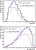 |
Fig. 1 Redshift and magnitude distributions of the quasars selected over Stripe 82 with the QSO_EBOSS_CORE (10 481 objects) or the QSO_VAR_S82 (16 243 objects) flag. |
For all the objects, the eBOSS pipeline encodes the spectrum classification into the CLASS_AUTO flag and the redshift, when relevant, into Z_AUTO. When the spectrum was visually inspected, two additional flags are set: CLASS_PERSON, which encodes the classification, and Z_CONF_PERSON, which encodes the confidence on the redshift estimate (Pâris et al. 2014). We define a spectrum “uberclass” as follows. If a visual inspection was done and led to a clear identification (Z_CONF_PERSON ≥ 2), then the object uberclass is set equal to CLASS_PERSON (i.e., Star, Quasar, or Galaxy). If visual inspection did not lead to a clear identification, the uberclass is set to “Inconclusive”. In the absence of visual inspection, the uberclass is set equal to CLASS_AUTO, which can also be Inconclusive. We define our sample of quasars as the set of targets with uberclass equal to Quasar. The quasar redshift is set equal to the visual inspection redshift if the latter is available and to Z_AUTO otherwise.
We illustrate in Fig. 1 the magnitude and redshift distributions of the quasars selected in Stripe 82 with the QSO_EBOSS_CORE or the QSO_VAR_S82 flag, including the known quasars (and the overlap with CORE in the variability sample). A large number of the quasars are common to both selections. The QSO_VAR_S82 sample, however, contains about 1.6 times more quasars than the QSO_EBOSS_CORE sample. The origin of this improvement is two-fold. Part of it is due to the fact that the QSO_VAR_S82 sample is selected from about 50 epochs of photometry, instead of a single epoch for the QSO_EBOSS_CORE sample (which is done to ensure the uniformity with the rest of the eBOSS footprint). The other part of the improvement comes from the different selection techniques: at identical depths for the input photometry, using for instance 50-epoch coadded images to measure object colors and 50 individual epochs of imaging to measure variability criteria, we have shown in Paper Var that the variability selection selects 30% more quasars than the CORE selection for the same total number of targets.
The QSO_VAR_S82 sample significantly increases the completeness at all redshifts and magnitudes and, in particular, at the faint end (g ~ 22−22.5). In the rest of this paper, we focus on the targets with the QSO_VAR_S82 bit set.
3. Data and target selection
This section provides an overview of the control sample of quasars used throughout this study. We present the imaging data from which the targets are selected, describe the selection algorithm, and discuss the spectroscopic survey. The magnitudes of the sources are denoted u, g, r, i, and z when referring to observed magnitudes, and udered, gdered, rdered, idered, and zdered when referring to magnitudes corrected for Galactic extinction using the extinctions from the maps of Schlegel et al. (1998). The bands correspond to the SDSS filters (Fukugita et al. 1996; Doi et al. 2010).
3.1. Control sample
The completeness corrections related to the criteria used to select the targets are determined using a control sample of 4555 spectroscopically confirmed quasars that were selected in Stripe 82 independently of any variability criterion. This prevents our control sample from being biased toward sources that exhibit high quasar-like variability. Such quasars would indeed have led to overly optimistic completeness estimates for our selection algorithm.
The control sample is built from the 2dF quasar catalog (Croom et al. 2004), the 2dF-SDSS LRG and Quasar Survey 2SLAQ (Croom et al. 2009), the SDSS-DR7 quasar catalog (Schneider et al. 2010), and BOSS observations through August 2010 (Ahn et al. 2012; Pâris et al. 2012). These catalogs were obtained from pure color selections (cf., for instance, Richards et al. 2002 for DR7 and Ross et al. 2012 for BOSS). BOSS observations taken after Summer 2010 on Stripe82 had contributions from a variability selection and were therefore discarded from the control sample.
Color information comes from flux ratios, so is not sensitive to absolute fluxes, while variability information comes from variations in absolute fluxes. Furthermore, time variations are seen to be synchronous in different bands, thus not affecting the source colors. Color and variability selections are therefore complementary, as already shown in Paper Var, with no obvious correlations between the photometric and time-domain characteristics of quasars. The only source of correlations could come from the image depth, but we take this into account by computing all corrections as a function of source magnitude. We thus expect no measurable bias in our completeness estimates from the use of this control sample.
3.2. Imaging data and target selection
The selection of the targets for this study relies heavily on the variability selection described in Paper Var where all the details can be found, so we only summarize the main steps here.
The initial source list is determined from the co-addition of single-epoch SDSS images (Annis et al. 2014) in Stripe 82, from which we take the source magnitude (in SDSS u, g, r, i and z bands) and morphology. As morphology indicator, we use a continuous variable defined as  (1)where mPSF(g) and mmodel(g) are the magnitudes of the source, measured in the g band, obtained from a PSF fit (valid for unresolved objects) or a model fit (more appropriate for extended objects, where model can be a de Vaucouleurs or an exponential shape, for instance), respectively. As shown in Fig. 2, mdiff peaks near 0 with a standard deviation of 0.01 for point-like sources, and extends from 0.01 to values beyond 0.3 for extended sources.
Because the emitting region of a quasar, which is too small to be resolved, outshines the host galaxy by a large factor, a quasar generally appears as a stellar-like source. Only for the nearest quasars (redshift z< 0.9 at most) can the host galaxy be detectable in co-added images, making the source appear extended in those cases (see Sect. 2.4 of Paper LF for a quantitative study of the effect). The average morphology indicator as a function of redshift for the quasars of the control sample is displayed in Fig. 3. It is at the level of 0.2 or more as the redshift approaches 0, has a value of about 0.1 at z ~ 0.5, and is below 0.05 for redshifts z> 0.6. At z> 2.5, the small decrease in mdiff with increasing redshift is correlated to the increasing average magnitude of the quasars. The larger the photometric errors, the less the PSF and model fits tend to capture a difference in spatial extension of the source, and the closer on average mdiff is to zero. We apply a cut on morphology (upper bound on mdiff, cf. details below) to reject galaxies.
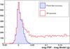 |
Fig. 2 Difference between PSF and model magnitudes, used as morphology indicator, for random objects in Stripe 82. Point-like sources in the co-added images, overlaid in blue, have a small magnitude difference. Quasar selection requires magnitude differences of at most 0.05, relaxed to 0.1 for objects with a high significance of quasar-like variability (to recover low-z quasars where the host galaxy can make the source appear extended). |
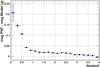 |
Fig. 3 Morphology indicator as a function of redshift for quasars. The cut at 0.05 includes most quasars at z> 0.6, but rejects most lower-redshift quasars whose host galaxy is detectable in co-added images. |
To reduce the stellar contamination, we apply a loose color cut by requiring that c3< 1−0.33 × c1, where c1 and c3 are defined as in Fan (1999) by 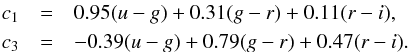 (2)This is the same criterion as was used in Paper LF, where we had estimated that close to 100% of z< 2.2 and 98% of z> 2.2 known quasars (i.e., quasars from the control sample of Sect. 3.1) passed that condition. The completeness of this color cut is included in the selection efficiency ϵsel described in Sect. 4.1.
The main selection is based upon a criterion measuring the variability with time of the source. The lightcurves of our sources contain, on average, 52 SDSS individual epochs spread over seven years. They are used to compute two sets of parameters that characterize the source variability:
-
the χ2 of the fit of the lightcurve in each of the ugriz filters by a constant
 :
: ![Mathematical equation: \hbox{$\chi^2 = \sum_i \left[(m_i - \overline{m}) / \sigma_i \right] ^2$}](/articles/aa/full_html/2016/03/aa27392-15/aa27392-15-eq71.png) , where the sum runs over all observations i;
, where the sum runs over all observations i; -
two parameters, an amplitude A, and a power γ as introduced by Schmidt et al. (2010), which characterize the variability structure function
 , i.e., the change in magnitude Δmij as a function of time lag Δtij for any pair ij of observations:
  . Because quasars have similar time variations in different bands, we reduce the uncertainty on variability parameters by fitting the g, r, and i bands simultaneously (those least affected by noise and observational limitations) for a common γ and independent amplitudes Ag, Ar, and Ai.
Variable objects, whether quasars or stars, are expected to have large χ2’s, thus allowing a distinction between variable and non-variable targets. The structure function parameters A and γ can distinguish between these two classes of variable objects: quasars tend to have both large A and large γ, due to magnitude changes that increase with time, while variable stars (such as pulsating or eclipsing binaries) can have large A but usually γ near 0.
For each source, a neural network combines the five χ2, the power γ, and the amplitudes Ag, Ar, and Ai to produce an estimate of quasar-like variability. The training of the NN was done using a large sample of 13 063 spectroscopically confirmed quasars with redshifts in 0.05 ≤ z ≤ 5.0 and magnitudes in the range 18 ≤ g ≤ 23, and a star sample consisting in 2609 objects spectroscopically confirmed as stars in the course of the BOSS project. The two samples are located in Stripe 82, and thus have identical time sampling characteristics to the present data. An output vNN of the neural network near 0 designates non-varying objects, as is the case for the vast majority of stars, while an output near 1 indicates lightcurves exhibiting quasar-like variability.
A source is selected according to its quasar-like variability (vNN) and morphology (mdiff). A loose morphology cut (mdiff< 0.1) is applied if the variability indicator is high (vNN> 0.85); a strict morphology cut (mdiff< 0.05) is applied in case of a lower variability indicator (0.50 <vNN< 0.81); and for values of vNN intermediate between 0.81 and 0.85, the threshold on mdiff is gradually evolved between the two extreme values of 0.05 and 0.1. Even the tightest bound (0.05) fully encompasses the range of potential values for point-like sources.
We restrict the study to sources with g< 22.8 and gdered< 22.5. The average g Galactic extinction over the observed zone of Stripe 82 is 0.12, so both limits are comparable. With this magnitude limit, the selection described above leads to a sample density of 175 deg-2 targets. Removing targets that already have a spectroscopic identification from previous observations reduces the sample to about 95 deg-2 targets. Further removing the overlap with the CORE sample (bit QSO_EBOSS_CORE) yields the target density of 50 deg-2 indicated in Table 1.
3.3. Spectroscopic data
The eBOSS footprint overlaps Stripe 82 over a total of 120 deg2 delimited by −3°<αJ2000< 45° and −1.25°<δJ2000< 1.25°. The first year of eBOSS observations led to the coverage illustrated in Fig. 4: dots indicate the position of quasars in plates that have been observed by eBOSS. Some outskirt regions (shown in gray in the figure) have less than 100% completeness because of overlapping plates that had not yet been observed at the time of this work. In the present analysis, we restrict ourselves to the region that has 100% completeness (in black in the figure). Its total area is 94.5 deg2.
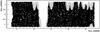 |
Fig. 4 Footprint of the first year of eBOSS observations used for this study (aspect ratio is not 1:1). Incomplete regions are shown in gray, fully observed ones in black. |
In the course of the BOSS survey, several ancillary projects have covered parts or all of Stripe 82, either to test target selection techniques (Paper Var from quasars targeted with BOSS chunk 11 over all Stripe 82), or as pilot programs for eBOSS and DESI (Ross et al. 2012; Dawson et al. 2013; Alam et al. 2015). In particular, three programs aimed to provide an exhaustive census of quasars to at least gdered ~ 22.5 in Stripe 82. The first one, conducted jointly in BOSS (chunk 21, target bit QSO_VAR_FPG) and on the Multiple Mirror Telescope, was done in the region delimited by 317°<αJ2000< 330°. It provided a total of nearly 1800 quasars at a mean magnitude ⟨ gdered ⟩ = 21.1 and led to the QLF paper mentioned previously (Paper LF). The other two programs were conducted in the region of Stripe 82 delimited by 36°<αJ2000< 42° where Galactic extinction is low (cf., DR12 release of SDSS-III: Alam et al. 2015): one program (BOSS chunk 205, target bit QSO_VAR_LF) identified about 1600 new quasars to gdered ~ 22.5, while the second (BOSS chunk 218, target bit QSO_DEEP), aimed at identifying fainter targets and provided an additional 363 quasars at ⟨ gdered ⟩ = 22.6. The QSO_VAR_LF and the QSO_DEEP programs more than doubled the density of known quasars given in Table 1 for the rest of Stripe 82. The 36°<αJ2000< 42° region of Stripe 82 where a deep quasar sample is available is used in this work to cross-check the completeness-corrected counts computed in Sect. 4.
4. Quasar number counts
We here compute the completeness corrections that affect our sample regardless of whether they are related to the analysis technique or to observational constraints. We present raw number counts derived from the observation of our targets and compute corrected number counts used in Sect. 5 to derive a quasar luminosity function. As mentioned above, we only give counts within the fully observed zone (black area in Fig. 4), of area 94.5 deg2.
4.1. Completeness corrections
We derive the spectroscopy-related completeness corrections from the data themselves, and the selection-related corrections from the application of the same selection cuts to the control sample of quasars. We describe the different contributions below.
Morphology completeness, ϵmorph(z,g)
As explained in Sect. 3.2, we only select targets among the sources that pass the morphology cut mdiff< 0.1. Therefore, sources that are more extended than allowed by this cut are not considered as possible candidates. Nevertheless, some low-redshift quasars for which the host galaxy is resolved can fail this criterion (cf., Fig. 2). We compute the correction related to this incompleteness by considering the fraction of the quasars in our control sample that have mdiff> 0.1 as a function of redshift and magnitude. This procedure underestimates the effect slightly, since the control sample dominantly consists of objects that were already selected as unresolved sources. The selection, however, was based on single-epoch photometry (and not on coadded images as for the present study), making it less sensitive to morphology than the current one. The morphology incompleteness 1 /ϵmorph is a factor ~1.7 at redshift z< 0.5, a factor 1.2 for z in 0.5−0.8, 1.1 for z in 0.8−1.0, and it is compatible with 1.0 for z> 1. We start our measurement of the quasar LF at z = 0.67, where the correction is at most ~10%.
Target selection completeness, ϵsel(g,mdiff)
The selection completeness is determined from the fraction of quasars in the control sample that pass the color and variability criteria of Sect. 3.2. The result is illustrated in Fig. 5 as a function of magnitude g and morphology mdiff. The efficiency drops for fainter objects where the variability signal is not as visible and for large mdiff because of the stricter variability cut applied to more extended objects. On average over the selected sample, the selection completeness is 0.86.
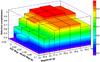 |
Fig. 5 Selection completeness ϵsel(g,mdiff) for quasars used in this study. The loss at large PSF-model magnitudes, i.e., more extended objects, is due to the more stringent cut on variability for such sources. The loss at large magnitudes is due to increased photometric dispersion in the lightcurves, which blurs the variability signal. |
Spectroscopic completeness, ϵspect(g)
Some spectra did not produce a reliable identification of the source, either because the extraction procedure failed (yielding flat and useless spectra) or because the spectrum had too low a signal-to-noise ratio (S/N) for adequate identification, whether at the pipeline or at the visual inspection level. As explained in Sect. 2, we generally consider such spectra as inconclusive. We make the assumption that the ratio of quasars to non-quasars in the identified and inconclusive sets are identical. This hypothesis is confirmed by the fact that the ensemble structure function parameters (globally accounted for by the vNN parameter) are similar for the two sets. There is a small trend for a higher fraction of non-quasars in the inconclusive sample as the magnitude increases beyond g ~ 22, but the effect is small. Furthermore, because the selection completeness drops much faster with magnitude than the spectroscopic completeness (cf. Fig. 8 for a comparative illustration), even a large change in the fraction of quasars in the inconclusive set (for instance from the current 80% at g ~ 22.5 to 50%) only affects the overall completeness at g ~ 22.5 by less than 3%.
We compute the spectroscopic completeness from the fraction of inconclusive spectra as a function of magnitude (cf. Fig. 6). This correction is only applied to new quasars since previously known ones are, by definition, spectroscopically identified. The completeness correction is 0.93 on average over the 7900 new quasars and 1 by definition for known quasars. As illustrated in Fig. 6, there is a constant ~1% fraction of inconclusive spectra at bright magnitudes. This fraction increases to 8% at g = 22, 16% at g = 22.5, and 30% at g = 23. By comparison, the measured fractions of inconclusive spectra are 3%, 8%, and 24% at g of 22, 22.5, and 23, respectively, in the BOSS+MMT program of Paper LF. Part of the difference can be explained by our now more being conservative in the identification procedure. With identical definitions of inconclusive spectra, the percentages are compatible for g> 22.5, but remain slightly higher for the current analysis at g< 22. Inspection of the inconclusive spectra at bright magnitudes indicates that most of them have a redshift around 0.7 where the automated pipeline is not yet fully optimized (focus for BOSS was on z> 2.2 quasars, and for eBOSS on z> 0.9 quasars, thus higher redshifts than where this artifact appears).
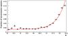 |
Fig. 6 Fraction of inconclusive spectra (i.e., 1−ϵspect(g)) as a function of observed g magnitude. The curve is an empirical fit to the data by a hyperbolic tangent. The ~1% loss at bright magnitudes is an artifact of the current pipeline. The increase at faint magnitudes is compatible with previous estimates. |
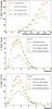 |
Fig. 7 Extinction-corrected magnitude (top) and redshift (middle and bottom) distributions. At faint magnitudes, most variability-selected sample (green triangles) comes from the newly identified quasars (open dark green triangles). The deep sample (orange circles) from the 36°<α< 42° zone (cf. Sect. 3.3) reproduces the corrected counts well (plain red circles) to g = 21.5, validating the computation of the completeness corrections to this magnitude limit. The deep sample is the only one to extend beyond g = 22.5. |
Tiling completeness, ϵtiling
Some spectroscopic targets cannot be observed either by lack of an available fiber on the plate (target density locally too high) or because a fiber cannot be placed at that plate position, for instance, because of fiber collisions. (Two fibers cannot be located less than 62′′ apart, cf. Dawson et al. 2013) This loss is random, independent of redshift or magnitude, and ϵtiling simply indicates the portion of the targets that were assigned fibers. It is equal to 0.959 for all new quasars and equal to 1 by definition for already known quasars.
4.2. Raw number counts
We identified 7900 new quasars and selected another 5976 that had been spectroscopically identified previously. The magnitude and redshift distributions of the quasars selected by this study are shown in Fig. 7 as the open dark green triangles for the new quasars and as the plain green triangles for the total sample of selected quasars including the already identified ones. The deep sample (cf., Sect. 3.3) is the only one to include quasars beyond gdered = 22.5.
As is clearly visible from Fig. 7, the newly identified quasars have a similar redshift distribution as the previously identified ones, but extend to fainter magnitudes on average, with ⟨ gdered ⟩ = 21.5 / 20.4 for the newly or previously identified quasars, respectively. Table 2 lists the raw quasar counts for this study in three bins of observed magnitude g. Our sample is particularly valuable at faint magnitudes: at g> 22, it increases the number of known quasars in the footprint by almost a factor of 6.
Raw number counts for the samples of new (“eBOSS”) and previously identified (“known”) quasars for the variability-selection of this study, in several g magnitude bins.
4.3. Corrected number counts
We derive corrected quasar number counts from raw number counts by accounting for the different sources of incompleteness detailed above. New quasars are corrected for morphology cut, target selection, tiling losses, and spectroscopic failures, while previously known quasars are only corrected for morphology and selection since their identification does not depend on eBOSS observation. The completeness-corrected number of quasars is thus given by  (3)The total completeness correction for new eBOSS quasars has an average of 0.70 and a standard deviation of 0.15, and for previously known quasars an average of 0.90 and a standard deviation of 0.12. The overall completeness of the full sample as a function of magnitude is illustrated in Fig. 8.
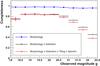 |
Fig. 8 Magnitude dependence of the contributions to the total completeness correction, averaged over all variability-selected quasars of the eBOSS and known samples. |
To validate the computation of the completeness corrections, it is interesting to compare the corrected quasar densities to the measurements done in the deep zone. Despite higher counts, it is clearly visible in Fig. 7 (top plot) that the deep region still suffers from significant incompleteness at gdered> 21.5. In Table 3, we therefore provide both the completeness-corrected densities to a limiting magnitude gdered< 21.5, where the deep sample is expected to be complete, and those to gdered< 22.5 from which we measure the quasar LF. At gdered< 21.5, the corrected counts and the deep sample show excellent consistency with less than 1.5σ deviations over the entire redshift range (Fig. 7, middle plot), which is compatible with Poisson errors. The magnitude distributions of the completeness-corrected and deep-zone counts (Fig. 7, top plot) are also in excellent agreement to gdered< 21.5. Extending the study to gdered< 22.5 (Table 3 or Fig. 7, bottom plot), the corrected counts are about 10% greater than the counts in the deep zone, a reasonable excess that is easily accounted for by the incompleteness of the deep sample at the faint end.
Areal densities (in deg-2) in several redshift bins for this work (after completeness correction) for the deep 36°<α< 42° zone (raw counts) and from the best-fit luminosity function of Paper LF.
Table 3 also lists the expected number counts from the luminosity function computed in Paper LF. The results from this new study show a small global increase of 10% to 20% in number counts over these previous estimates. As explained above, the completeness-corrected densities measured in this work agree with the deep-zone raw counts at the bright end and show a 10% understandable excess at the faint end. Furthermore, the deep sample gives a solid lower bound on quasar densities. For these reasons, we are confident that the discrepancy between the two studies is due to slightly underestimated completeness corrections in Paper LF, rather than overestimated corrections in the present work. Given that the total corrections in Paper LF ranged from 1.2 at g< 20 to a factor 2 at g ~ 22.5, a 10% inaccuracy is not surprising.
5. Luminosity function in g
We derive the QLF in a similar manner to what was described in Paper LF. We compute a binned QLF from the corrected number counts of Sect. 4.3, considering our completeness limit at gdered = 22.5. We fit two parametric models to our binned QLF and compare the number counts each model predicts over the range of magnitude and redshift observable by eBOSS. Finally, we use our QLF fits to predict number counts to fainter magnitudes than achieved by eBOSS, as needed for future quasar surveys.
5.1. Binned luminosity function
Selection for this survey was performed in the g-band, which provides the highest S/N for a vast fraction of the data. For each quasar, we compute the absolute magnitude normalized to z = 2 by ![Mathematical equation: \begin{equation} M_g(z\!=\!2) = g_{\rm dered}-d_M(z)-[K(z)-K(z\!=\!2)], \end{equation}](/articles/aa/full_html/2016/03/aa27392-15/aa27392-15-eq154.png) (4)where the distance modulus dM(z) is computed assuming a flat ΛCDM cosmology with (ΩΛ,ΩM,w,h) = (0.6935,0.3065,−1,0.679), as measured by the Planck Collaboration et al. (2015) in the “TT+lowP+lensing+ext” configuration, and K(z) is the K correction that accounts for redshifting of the bandpass of the spectrum. We have chosen to normalize the magnitudes at z = 2, because it is close to the median redshift of our sample, and it allows backward compatibility with previous studies (Croom et al. 2009; Ross et al. 2013; Palanque-Delabrouille et al. 2013). As in Paper LF, we use the K correction as a function of redshift that was derived by McGreer et al. (2013) following a similar approach to the one in Richards et al. (2009). As illustrated in Fig. 9, the K correction is close to that of Croom et al. (2009) for z< 3, but extends to higher redshifts. It varies with luminosity owing to the accounting of strong quasar emission lines whose equivalent widths are a function of luminosity (Baldwin 1977). This luminosity dependence introduces a spread of ~0.25 mag at z ~ 2−3 where the Lyman-α and C-IV lines contribute substantially to the flux in g band.
(4)where the distance modulus dM(z) is computed assuming a flat ΛCDM cosmology with (ΩΛ,ΩM,w,h) = (0.6935,0.3065,−1,0.679), as measured by the Planck Collaboration et al. (2015) in the “TT+lowP+lensing+ext” configuration, and K(z) is the K correction that accounts for redshifting of the bandpass of the spectrum. We have chosen to normalize the magnitudes at z = 2, because it is close to the median redshift of our sample, and it allows backward compatibility with previous studies (Croom et al. 2009; Ross et al. 2013; Palanque-Delabrouille et al. 2013). As in Paper LF, we use the K correction as a function of redshift that was derived by McGreer et al. (2013) following a similar approach to the one in Richards et al. (2009). As illustrated in Fig. 9, the K correction is close to that of Croom et al. (2009) for z< 3, but extends to higher redshifts. It varies with luminosity owing to the accounting of strong quasar emission lines whose equivalent widths are a function of luminosity (Baldwin 1977). This luminosity dependence introduces a spread of ~0.25 mag at z ~ 2−3 where the Lyman-α and C-IV lines contribute substantially to the flux in g band.
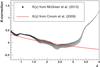 |
Fig. 9 The g-band K-correction as a function of redshift. The spread illustrates the luminosity variation of the correction for the quasars in our sample. The sudden change at z> 3 is due to the suppression of the flux in g band by the intervening Lyman-α absorbers. |
We define eight redshift bins with limits 0.68, 1.06, 1.44, 1.82, 2.2, 2.6, 3.0, 3.5, and 4.0. The binned LF is computed for each redshift using the model-weighted estimator Φ suggested by Miyaji et al. (2001) and used in previous studies such as in Croom et al. (2009) or in Paper LF. The binned LF is given by  (5)where Mgi and zi are, respectively, the absolute magnitude and the redshift at the center of bin i, Φmodel is the model LF estimated at the center of the bin,
  is the number of quasars in the bin with gdered< 22.5 estimated from the model, and
  is the observed number of quasars in the bin. This estimator is free from most of the biases that are unavoidable in the more usual 1 /V method devised by Page & Carrera (2000), and improves upon it in several ways. It corrects for variations in the LF within a bin (particularly critical at the steep bright end of the QLF), corrects for incompleteness in a bin (particularly critical at the faint end of our LF where the bin is incompletely sampled), and allows exact errors to be evaluated using Poisson statistics. A drawback of this estimator is that it is model-dependent, but Miyaji et al. (2001) demonstrate that the uncertainties due to the model dependence are practically negligible. We free ourselves here of any model dependence by performing an iterative fitting to determine the binned QLF from Eq. (5) and our choice of model, until parameter convergence is reached. As explained in the following section, we use two different models to fit the QLF, which do not produce any significant difference to the estimate of the binned LF.
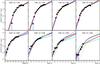 |
Fig. 10 Quasar luminosity function measurements (black circles). The best-fit models of this work are shown as the red (respectively blue) curves for the PLE+LEDE (resp. PLE) models. The green dot-dashed curve is the LF of Croom et al. (2009). The plain cyan curve is the best fit LEDE model of Ross et al. (2013) at z> 2.2. The orange dotted and dashed curves are the best fits to COSMOS data (Masters et al. 2012) at z ~ 3.2 (shown in the last two redshift bins) and z ~ 4.0, respectively. The magenta dashed curve (almost exactly overlapping the orange dotted curve at the faint end in the 3.0 <z< 3.5 redshift bin) is measured at z ~ 3.2 from SWIRE and SDSS (Siana et al. 2008). |
5.2. QLF model fits
The QLF is traditionally fit by a double power law of the form (Boyle et al. 2000; Richards et al. 2006):  (6)where Φ is the quasar comoving space density and
  a characteristic, or break, magnitude. The slopes α and β describe the evolution of the LF on either side of the break magnitude. In this work, we consider two extensions of this simple form described below.
Our first model is the same as the one we used in Paper LF. We consider a pure luminosity-evolution (PLE) model as in Croom et al. (2009), where a redshift dependence of the luminosity is introduced through an evolution in described by ![Mathematical equation: \begin{equation} M_g^*(z)=M_g^*(z_{\rm p})-2.5\left[k_1(z-z_{\rm p})+k_2 (z-z_{\rm p})^2\right] . \label{eq:mg} \end{equation}](/articles/aa/full_html/2016/03/aa27392-15/aa27392-15-eq211.png) (7)We allow the redshift-evolution parameters (k1 and k2) and the model slopes (α and β) to be different on either side of a pivot redshift zp = 2.2. The model is thus described by Eqs. (6) and (7) where α, β, k1, and k2 are defined with subscript l for z<zp and h for z>zp. This PLE model therefore has ten parameters (Φ∗,
(7)We allow the redshift-evolution parameters (k1 and k2) and the model slopes (α and β) to be different on either side of a pivot redshift zp = 2.2. The model is thus described by Eqs. (6) and (7) where α, β, k1, and k2 are defined with subscript l for z<zp and h for z>zp. This PLE model therefore has ten parameters (Φ∗,  , αl, βl, k1l, k2l, αh, βh, k1h, and k2h) that are free to vary in the fit.
An extensive study of the QLF was performed by Ross et al. (2013) on 23 300 quasars with i< 21.8 and 2.2 <z< 3.5 from the DR9 release of BOSS data (Ahn et al. 2012), complemented by about 5500 quasars over 2.2 <z< 3.5 from Paper Var and about 1900 quasars over 0.3 <z< 3.5 from Paper LF. The authors showed that a good fit to this large sample of quasars over the full redshift range was obtained by using a PLE model for z< 2.2, and a model with both luminosity and density evolution (LEDE) for z> 2.2, where the normalization and break magnitude evolve in a log-linear manner, e.g.,
![Mathematical equation: \begin{eqnarray} &&\log[\Phi^*(z)]=\log[\Phi^*(z_{\rm p})]+c_{1a}(z-z_{\rm p})+c_{1b}(z-z_{\rm p})^2\\ &&M_g^*(z)=M_g^*(z_{\rm p})+c_2(z-z_{\rm p})\label{eq:mg_LEDE} \end{eqnarray}](/articles/aa/full_html/2016/03/aa27392-15/aa27392-15-eq231.png) with zp = 2.2 the pivot redshift. This PLE (for z< 2.2) + LEDE (for z> 2.2) is our second model where we fit our binned QLF. Unlike Ross et al. (2013), however, we impose continuity of the LF at z = zp by requiring the same normalization Φ∗(zp) and break magnitude for both the PLE and the LEDE forms. We allow for some additional flexibility by allowing a redshift dependence of the slope, according to
with zp = 2.2 the pivot redshift. This PLE (for z< 2.2) + LEDE (for z> 2.2) is our second model where we fit our binned QLF. Unlike Ross et al. (2013), however, we impose continuity of the LF at z = zp by requiring the same normalization Φ∗(zp) and break magnitude for both the PLE and the LEDE forms. We allow for some additional flexibility by allowing a redshift dependence of the slope, according to 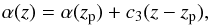 (10)where α(zp) is equal to the value of α used at z<zp in the PLE form. Our PLE+LEDE model therefore has ten parameters (Φ∗(0),
  , α(zp), β(zp), k1, k2, c1a, c1b, c2, and c3) that are left free to vary in the fit.
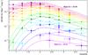 |
Fig. 11 . Comparison of our best-fit PLE+LEDE model (solid curves) to the eBOSS Stripe 82 QLF data (points). From bottom to top, the curves correspond to magnitudes MG(z = 2) = −28.4, −28, −27.6, −27.2, −26.8, −26.4, −26, −25.6, −25.2, −24.8, −24.2, −24, and −23.6. A simple PLE model breaks down at z = 2.2. Here, we switch to an LEDE model at z> 2.2. The mixed PLE+LEDE model reproduces the QLF well. |
The best-fit parameters are given in Table 4. Both models have ten parameters free to vary in the fit, and start with 100 data points spread over eight redshift bins. Throughout the iterations (ten are needed in both cases to reach parameter convergence), the QLF is recomputed according to Eq. (5), and points that are corrected by more than a factor 2 (owing to the incompleteness introduced by the gdered< 22.5 cut) are removed from the fit. One to two points per redshift bin are excluded by this procedure. The resulting best-fit models are illustrated in Fig. 10, along with the best-fit model obtained by Croom et al. (2009) for z< 2.2 and extrapolated to higher redshift, and the PLE+LEDE model of Ross et al. (2013) shown for z> 2.2, where it is best constrained by the DR9 data used for the fit. In the z< 2.2 range, our two models are in excellent agreement with Croom et al. (2009), and are a good fit to our binned QLF. At z> 2.2, our two models show similar trends at the bright end, but start to differ at the faint end of the QLF, in particular for the highest two redshift bins, which are lacking faint quasars. The agreement with Ross et al. (2013) is good over the common redshift range, but the fits also start to deviate at z> 3.5 where data are scarce. Although we constrain our models to be continuous at z = 2.2, the fit reduced χ2s are less than 2. Such values were only obtained in Ross et al. (2013) when fitting over restricted redshift ranges, typically limiting to data below or above a redshift of 2.2. Figure 11 presents the redshift evolution of the QLF in a series of luminosity bins, including both our data and the best-fit PLE+LEDE model. The “kink” at z = 2.2 is due to the change of analytical form at this pivot redshift. The model, however, is continuous at z = 2.2.
We provide, in Appendix A, the measured luminosity function values and associated uncertainties, where the measurements were corrected using the model-weighted estimator of Eq. (5) and considering the best-fit PLE+LEDE model.
Quasar densities (in deg-2) predicted from the two phenomenological models of this study.
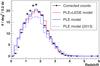 |
Fig. 12 Projected counts for gc< 22.5 for the PLE (blue) and the PLE+LEDE (red) luminosity function models used to fit the binned QLF. The dashed curve is the best-fit model of Paper LF, shown here for comparison. Our new fits indicate a ~10% increase in total quasar counts. |
Predicted differential quasar counts over 15.5 < g < 25 and 0 < z < 6 for a survey covering 10 000 deg2, based on our best-fit PLE or PLE+LEDE luminosity function model.
5.3. Predicted number counts
Out best-fit luminosity functions can be used to estimate the density of quasars as a function of redshift and magnitude. As shown in Table 5, the redshift distributions predicted by our two models agree within 0.3% for counts to a limiting magnitude g< 22.5 and within 1.1% to g< 23. The largest discrepancy between the models occurs near z = 2.3 (cf. Fig. 12), close to the pivot redshift zp = 2.2 where the analytical form of our models changes, causing a small discontinuity in the derivative of their redshift evolution. At z ~ 2.3, the predictions from the two models differ by about 10%.
The two models are also in good agreement with the corrected number counts of Sect. 4.3 (Table 3) and indicate a ~15% increase over previous estimates based on the QLF fit of Paper LF. Both the PLE and the PLE+LEDE models fit the z> 2 data well, but do not provide as good a fit to the z< 0.6 range. A possible explanation for this discrepancy is a loss of low-z quasars in our selection, possibly because of the morphology cut for which the completeness efficiency ϵmorph does not account sufficiently. Another possibility is the misidentification of low-z quasars with the current pipeline (cf. paragraph on spectroscopic completeness in Sect. 4.1). This small discrepancy, however, is of little relevance for large-scale spectroscopic surveys that are mostly focusing on quasars at z> 1 where they are abundant enough to probe matter clustering.
Using the average g−r vs. redshift dependence that we measure for all DR12Q BOSS quasars, we can also calculate the number of quasars as a function of r-band magnitude. We provide these estimates for our two models as a function of g in Table 6 and as a function of r in Table 7, for a hypothetical survey covering 10 000 deg2.
Predicted differential quasar counts over 15.5 <r< 24 and 0 <z< 6 for a survey covering 10 000 deg2, based on our best-fit PLE or PLE+LEDE luminosity function model.
We can apply our best-fit QLF to future surveys, such as the third-generation large-scale spectroscopic survey DESI that aims to observe quasars to a limiting magnitude g = 23, or possibly r = 23 (to recover quasars at z> 3.6 that are g-band dropouts due to the absorption of their flux by Lyman-α absorbers along the line of sight). Expected quasar densities at DESI depth for our two models are given in the last two sections of Table 5. The 0.9 <z< 2.1 redshift range is where quasars are currently used as direct tracers of dark matter, and the z> 2.1 regime is where quasars are used to probe dark matter though the Lyman-α forest. The r< 23 limit produces slightly higher estimates than at g< 23, because quasars have positive g−r values at all redshift (g−r in 0.1−0.5 for z< 3.5, and increasing at higher redshift). Despite the differences between the PLE and the PLE+LEDE models that are visible in Fig. 10 or in the predicted counts of Tables 6 and 7 for faint magnitudes in particular, the density of quasars predicted by either model over the redshift and magnitude ranges of next-generation surveys are in excellent agreement at the 1.1% level for g< 23 and the 2.5% level for r< 23 in total quasar counts.
6. Conclusions
The extended Baryon Oscillation Spectroscopic Survey (eBOSS), part of the fourth iteration of the Sloan Digital Sky Survey, has an extensive spectroscopic quasar program that combines several selection techniques. Algorithms using the variability of quasar luminosity with time have been shown to be highly efficient to obtain large and complete samples of quasars.
Here we have presented the use in eBOSS of time-domain variability and focused on a specific program in Stripe 82 that led to a sample of 13,876 quasars to gdered = 22.5 over a 94.5 deg2 region, 1.5 times denser than expected to be obtained over the rest of the eBOSS footprint. This variability program provides a homogeneous and highly complete sample of quasars that is denser and greater in depth than samples that were used in previous studies dedicated to QLF measurements, such asCroom et al. (2009), Palanque-Delabrouille et al. (2013), and Ross et al. (2013). Using the data themselves, plus an external control sample of quasars selected with an independent (color-based) technique, we computed completeness corrections to account for quasar losses in the selection procedure, in the tiling, or in the spectroscopic identification.
We used this sample to measure the QLF in eight redshift bins from 0.68 to 4.0, and over magnitudes ranging from Mg(z = 2) = −26.60 to −21.80 at low redshift, and from Mg(z = 2) = −29.00 to −26.20 at high redshift. The data indicate a break at pivot redshift zp = 2.2, with a rise in luminosity followed by a steep decline as the redshift increases on either side of zp. The data are well fit by a double power-law model. We compared two models that we constrained to be continuous at zp: a quadratic PLE model as in Palanque-Delabrouille et al. (2013), with bright-end and faint-end slopes allowed to be different on either side of zp, and a PLE + LEDE model as in Ross et al. (2013), where a simple linear PLE is used for z< 2.2 and a LEDE with quadratic magnitude evolution is used at z> 2.2. These models both have ten parameters free to vary, and they fit the measured binned QLF equally well. Our models are in excellent agreement with Croom et al. (2009) at z< 2.2, and with Masters et al. (2012) at z> 2.2. Our two models start to deviate from one another in the highest two redshift bins (z> 3.0), although they both are in reasonable agreement with other measurements (Siana et al. 2008; Masters et al. 2012; Ross et al. 2013).
We used our models to predict densities of quasars for future quasar spectroscopic surveys. We predict 266 ± 3 deg-2 quasars to g< 23, and 304 ± 7 deg-2 quasars to r< 23, where the estimate is the mean of the two model estimates and the uncertainty is the difference between the estimate from either model and the mean.
Acknowledgments
Funding for the Sloan Digital Sky Survey IV has been provided by the Alfred P. Sloan Foundation, the U.S. Department of Energy Office of Science, and the Participating Institutions. SDSS-IV acknowledges support and resources from the Center for High-Performance Computing at the University of Utah. The SDSS web site is www.sdss.org. SDSS-IV is managed by the Astrophysical Research Consortium for the Participating Institutions of the SDSS Collaboration including the Brazilian Participation Group, the Carnegie Institution for Science, Carnegie Mellon University, the Chilean Participation Group, the French Participation Group, Harvard-Smithsonian Center for Astrophysics, Instituto de Astrofísica de Canarias, The Johns Hopkins University, Kavli Institute for the Physics and Mathematics of the Universe (IPMU)/University of Tokyo, Lawrence Berkeley National Laboratory, Leibniz Institut für Astrophysik Potsdam (AIP), Max-Planck-Institut für Astronomie (MPIA Heidelberg), Max-Planck-Institut für Astrophysik (MPA Garching), Max-Planck-Institut für Extraterrestrische Physik (MPE), National Astronomical Observatory of China, New Mexico State University, New York University, University of Notre Dame, Observatário Nacional/MCTI, The Ohio State University, Pennsylvania State University, Shanghai Astronomical Observatory, United Kingdom Participation Group, Universidad Nacional Autónoma de México, University of Arizona, University of Colorado Boulder, University of Portsmouth, University of Utah, University of Virginia, University of Washington, University of Wisconsin, Vanderbilt University, and Yale University. We acknowledge D. Vilanova for his help in the selection of the quasar targets with the variability algorithm.
References
- Ahn, C. P., Alexandroff, R., Allen de Prieto, C., et al. 2012, ApJSS, 203, 21 [NASA ADS] [CrossRef] [Google Scholar]
- Alam, S., Albareti, F. D., Allen de Prieto, C., et al. 2015, ApJS, 219, 12 [NASA ADS] [CrossRef] [Google Scholar]
- Annis, J., Soares-Santos, M., Strauss, M. A., et al. 2014, ApJ, 794, 120 [NASA ADS] [CrossRef] [Google Scholar]
- Baldwin, J. A. 1977, ApJ, 214, 679 [NASA ADS] [CrossRef] [Google Scholar]
- Bolton, A. S., Schlegel, D. J., Aubourg, E., et al. 2012, AJ, 144, 144 [NASA ADS] [CrossRef] [Google Scholar]
- Boyle, B. J., Shanks, T., & Peterson, B. A. 1988, MNRAS, 235, 935 [NASA ADS] [Google Scholar]
- Boyle, B. J., Shanks, T., Croom, S. M., et al. 2000, MNRAS, 317, 1014 [NASA ADS] [CrossRef] [Google Scholar]
- Busca, N. G., Delubac, T., Rich, J., et al. 2013, A&A, 552, A96 [NASA ADS] [CrossRef] [EDP Sciences] [Google Scholar]
- Croom, S. M., Richards, G. T., Shanks, T., et al. 2009, MNRAS, 392, 19 [NASA ADS] [CrossRef] [Google Scholar]
- Croom, S. M., Shanks, T., Boyle, B. J., et al. 2001, MNRAS, 325, 483 [NASA ADS] [CrossRef] [Google Scholar]
- Croom, S. M., Smith, R. J., Boyle, B. J., et al. 2004, MNRAS, 349, 1397 [NASA ADS] [CrossRef] [Google Scholar]
- Dawson, K. S., Schlegel, D. J., Ahn, C. P., et al. 2013, AJ, 145, 10 [Google Scholar]
- Delubac, T., Bautista, J. E., Busca, N. G., et al. 2015, A&A, 574, A59 [NASA ADS] [CrossRef] [EDP Sciences] [Google Scholar]
- Doi, M., Tanaka, M., Fukugita, M., et al. 2010, AJ, 139, 1628 [NASA ADS] [CrossRef] [Google Scholar]
- Eisenstein, D. J., Zehavi, I., Hogg, D. W., et al. 2005, ApJ, 633, 560 [NASA ADS] [CrossRef] [Google Scholar]
- Eisenstein, D. J., Weinberg, D. H., Agol, E., et al. 2011, AJ, 142, 72 [Google Scholar]
- Fan, X. 1999, AJ, 117, 2528 [NASA ADS] [CrossRef] [Google Scholar]
- Fan, X., Strauss, M. A., Schneider, D. P., et al. 2001, AJ, 121, 54 [NASA ADS] [CrossRef] [Google Scholar]
- Fukugita, M., Ichikawa, T., Gunn, J. E., et al. 1996, AJ, 111, 1748 [NASA ADS] [CrossRef] [Google Scholar]
- Gunn, J. E., Siegmund, W. A., Mannery, E. J., et al. 2006, AJ, 131, 2332 [NASA ADS] [CrossRef] [Google Scholar]
- Hasinger, G., Miyaji, T., & Schmidt, M. 2005, A&A, 441, 417 [NASA ADS] [CrossRef] [EDP Sciences] [Google Scholar]
- Hopkins, P. F., Richards, G. T., & Hernquist, L. 2007, ApJ, 654, 731 [NASA ADS] [CrossRef] [Google Scholar]
- Koo, D. C., & Kron, R. G. 1988, ApJ, 325, 92 [NASA ADS] [CrossRef] [Google Scholar]
- Law, N. M., Kulkarni, S. R., Dekany, R. G., et al. 2009, PASP, 121, 1395 [NASA ADS] [CrossRef] [Google Scholar]
- Masters, D., Capak, P., Salvato, M., et al. 2012, ApJ, 755, 169 [NASA ADS] [CrossRef] [Google Scholar]
- McGreer, I. D., Jiang, L., Fan, X., et al. 2013, ApJ, 768, 105 [NASA ADS] [CrossRef] [Google Scholar]
- Miyaji, T., Hasinger, G., & Schmidt, M. 2001, A&A, 369, 49 [NASA ADS] [CrossRef] [EDP Sciences] [Google Scholar]
- Page, M. J., & Carrera, F. J. 2000, MNRAS, 311, 433 [NASA ADS] [CrossRef] [Google Scholar]
- Palanque-Delabrouille, N., Yeche, C., Myers, A. D., et al. 2011, A&A, 530, A122 [NASA ADS] [CrossRef] [EDP Sciences] [Google Scholar]
- Palanque-Delabrouille, N., Magneville, C., Yèche, C., et al. 2013, A&A, 551, A29 [NASA ADS] [CrossRef] [EDP Sciences] [Google Scholar]
- Pâris, I., Petitjean, P., Aubourg, E., et al. 2012, A&A, 548, A66 [NASA ADS] [CrossRef] [EDP Sciences] [Google Scholar]
- Pâris, I., Petitjean, P., Aubourg, É., et al. 2014, A&A, 563, A54 [NASA ADS] [CrossRef] [EDP Sciences] [Google Scholar]
- Planck Collaboration 2015, A&A, submitted [arXiv:1502.01589] [Google Scholar]
- Rau, A., Kulkarni, S. R., Law, N. M., et al. 2009, PASP, 121, 1334 [NASA ADS] [CrossRef] [Google Scholar]
- Richards, G. T., Fan, X., Newberg, H. J., et al. 2002, AJ, 123, 2945 [NASA ADS] [CrossRef] [Google Scholar]
- Richards, G. T., Croom, S. M., Anderson, S. F., et al. 2005, MNRAS, 360, 839 [NASA ADS] [CrossRef] [Google Scholar]
- Richards, G. T., Myers, A. D., Gray, A. G., et al. 2009, ApJS, 180, 67 [NASA ADS] [CrossRef] [Google Scholar]
- Richards, G. T., Strauss, M. A., Fan, X., et al. 2006, AJ, 131, 2766 [NASA ADS] [CrossRef] [Google Scholar]
- Ross, N. P., Myers, A. D., Sheldon, E. S., et al. 2012, ApJS, 199, 3 [NASA ADS] [CrossRef] [Google Scholar]
- Ross, N. P., McGreer, I. D., White, M., et al. 2013, ApJ, 773, 14 [NASA ADS] [CrossRef] [Google Scholar]
- Schlegel, D. J., Finkbeiner, D. P., & Davis, M. 1998, ApJ, 500, 525 [NASA ADS] [CrossRef] [Google Scholar]
- Schlegel, D., Abdalla, F., Abraham, T., et al. 2011, ArXiv e-prints [arXiv:1106.1706] [Google Scholar]
- Schmidt, M., & Green, R. F. 1983, ApJ, 269, 352 [NASA ADS] [CrossRef] [Google Scholar]
- Schmidt, K. B., Marshall, P. J., Rix, H.-W., et al. 2010, ApJ, 714, 1194 [NASA ADS] [CrossRef] [Google Scholar]
- Schneider, D. P., Richards, G. T., Hall, P. B., et al. 2010, AJ, 139, 2360 [NASA ADS] [CrossRef] [Google Scholar]
- Siana, B., Polletta, M. D. C., Smith, H. E., et al. 2008, ApJ, 675, 49 [NASA ADS] [CrossRef] [Google Scholar]
- Slosar, A., Iršič, V., Kirkby, D., et al. 2013, J. Cosmol. Astropart. Phys., 2013, 026 [Google Scholar]
- Smee, S. A., Gunn, J. E., Uomoto, A., et al. 2013, AJ, 146, 32 [Google Scholar]
- Stoughton, C., Lupton, R. H., Bernardi, M., et al. 2002, AJ, 123, 485 [NASA ADS] [CrossRef] [Google Scholar]
- Tinker, J., & SDSS-IV Collaboration. 2015, in Am. Astron. Soc. Meet. Abstracts, 225, #125.06 [Google Scholar]
- York, D. G., Adelman, J., Anderson, Jr., J. E., et al. 2000, AJ, 120, 1579 [Google Scholar]
Appendix A
Table A.1 provides the binned luminosity function measured in this work using the model-weighted estimator described in Sect. 5.2, and plotted in Fig. 10. The table lists the value of log Φ in eight intervals spanning redshifts from z = 0.68 to z = 4.00,
and for ΔMg = 0.40 magnitude bins from Mg = −29.00 to Mg = −20.60. We also give the number of quasars (NQ) contributing to the LF in each bin, and the uncertainty (Δlog Φ). Bins with quasars but no corresponding value of the binned QLF are data points that were removed in the iterative fitting procedure owing to large correction factors.
Binned quasar luminosity function.
All Tables
eBOSS quasar targeting bits and average targeting densities in Stripe 82 except for PTF (densities over all footprint for PTF).
Raw number counts for the samples of new (“eBOSS”) and previously identified (“known”) quasars for the variability-selection of this study, in several g magnitude bins.
Areal densities (in deg-2) in several redshift bins for this work (after completeness correction) for the deep 36°<α< 42° zone (raw counts) and from the best-fit luminosity function of Paper LF.
Quasar densities (in deg-2) predicted from the two phenomenological models of this study.
Predicted differential quasar counts over 15.5 < g < 25 and 0 < z < 6 for a survey covering 10 000 deg2, based on our best-fit PLE or PLE+LEDE luminosity function model.
Predicted differential quasar counts over 15.5 <r< 24 and 0 <z< 6 for a survey covering 10 000 deg2, based on our best-fit PLE or PLE+LEDE luminosity function model.
All Figures
|
Fig. 1 Redshift and magnitude distributions of the quasars selected over Stripe 82 with the QSO_EBOSS_CORE (10 481 objects) or the QSO_VAR_S82 (16 243 objects) flag. |
| In the text | |
|
Fig. 2 Difference between PSF and model magnitudes, used as morphology indicator, for random objects in Stripe 82. Point-like sources in the co-added images, overlaid in blue, have a small magnitude difference. Quasar selection requires magnitude differences of at most 0.05, relaxed to 0.1 for objects with a high significance of quasar-like variability (to recover low-z quasars where the host galaxy can make the source appear extended). |
| In the text | |
|
Fig. 3 Morphology indicator as a function of redshift for quasars. The cut at 0.05 includes most quasars at z> 0.6, but rejects most lower-redshift quasars whose host galaxy is detectable in co-added images. |
| In the text | |
|
Fig. 4 Footprint of the first year of eBOSS observations used for this study (aspect ratio is not 1:1). Incomplete regions are shown in gray, fully observed ones in black. |
| In the text | |
|
Fig. 5 Selection completeness ϵsel(g,mdiff) for quasars used in this study. The loss at large PSF-model magnitudes, i.e., more extended objects, is due to the more stringent cut on variability for such sources. The loss at large magnitudes is due to increased photometric dispersion in the lightcurves, which blurs the variability signal. |
| In the text | |
|
Fig. 6 Fraction of inconclusive spectra (i.e., 1−ϵspect(g)) as a function of observed g magnitude. The curve is an empirical fit to the data by a hyperbolic tangent. The ~1% loss at bright magnitudes is an artifact of the current pipeline. The increase at faint magnitudes is compatible with previous estimates. |
| In the text | |
|
Fig. 7 Extinction-corrected magnitude (top) and redshift (middle and bottom) distributions. At faint magnitudes, most variability-selected sample (green triangles) comes from the newly identified quasars (open dark green triangles). The deep sample (orange circles) from the 36°<α< 42° zone (cf. Sect. 3.3) reproduces the corrected counts well (plain red circles) to g = 21.5, validating the computation of the completeness corrections to this magnitude limit. The deep sample is the only one to extend beyond g = 22.5. |
| In the text | |
|
Fig. 8 Magnitude dependence of the contributions to the total completeness correction, averaged over all variability-selected quasars of the eBOSS and known samples. |
| In the text | |
|
Fig. 9 The g-band K-correction as a function of redshift. The spread illustrates the luminosity variation of the correction for the quasars in our sample. The sudden change at z> 3 is due to the suppression of the flux in g band by the intervening Lyman-α absorbers. |
| In the text | |
|
Fig. 10 Quasar luminosity function measurements (black circles). The best-fit models of this work are shown as the red (respectively blue) curves for the PLE+LEDE (resp. PLE) models. The green dot-dashed curve is the LF of Croom et al. (2009). The plain cyan curve is the best fit LEDE model of Ross et al. (2013) at z> 2.2. The orange dotted and dashed curves are the best fits to COSMOS data (Masters et al. 2012) at z ~ 3.2 (shown in the last two redshift bins) and z ~ 4.0, respectively. The magenta dashed curve (almost exactly overlapping the orange dotted curve at the faint end in the 3.0 <z< 3.5 redshift bin) is measured at z ~ 3.2 from SWIRE and SDSS (Siana et al. 2008). |
| In the text | |
|
Fig. 11 . Comparison of our best-fit PLE+LEDE model (solid curves) to the eBOSS Stripe 82 QLF data (points). From bottom to top, the curves correspond to magnitudes MG(z = 2) = −28.4, −28, −27.6, −27.2, −26.8, −26.4, −26, −25.6, −25.2, −24.8, −24.2, −24, and −23.6. A simple PLE model breaks down at z = 2.2. Here, we switch to an LEDE model at z> 2.2. The mixed PLE+LEDE model reproduces the QLF well. |
| In the text | |
|
Fig. 12 Projected counts for gc< 22.5 for the PLE (blue) and the PLE+LEDE (red) luminosity function models used to fit the binned QLF. The dashed curve is the best-fit model of Paper LF, shown here for comparison. Our new fits indicate a ~10% increase in total quasar counts. |
| In the text | |
Current usage metrics show cumulative count of Article Views (full-text article views including HTML views, PDF and ePub downloads, according to the available data) and Abstracts Views on Vision4Press platform.
Data correspond to usage on the plateform after 2015. The current usage metrics is available 48-96 hours after online publication and is updated daily on week days.
Initial download of the metrics may take a while.