| Issue |
A&A
Volume 587, March 2016
|
|
|---|---|---|
| Article Number | A25 | |
| Number of page(s) | 14 | |
| Section | Extragalactic astronomy | |
| DOI | https://doi.org/10.1051/0004-6361/201527244 | |
| Published online | 16 February 2016 | |
Origin of X-shaped radio-sources: further insights from the properties of their host galaxies
1
Dipartimento di FisicaUniversità degli Studi di Torino,
via Pietro Giuria 1,
10125
Torino,
Italy
e-mail:
capetti@oato.inaf.it
2
School of Physics and Astronomy, University of
Birmingham, Edgbaston, Birmingham
B15 2TT,
UK
3
INAF – Osservatorio Astrofisico di Torino, via Osservatorio
20, 10025
Pino Torinese,
Italy
Received: 25 August 2015
Accepted: 8 December 2015
We analyze the properties of a sample of X-shaped radio-sources (XRSs). These objects show, in addition to the main lobes, a pair of wings that produce their peculiar radio morphology. We obtain our sample by selecting from the initial list of Cheung (2007, AJ, 133, 2097) the 53 galaxies with the better defined wings and with available SDSS images. We identify the host galaxies and measure their optical position angle, obtaining a positive result in 22 cases. The orientation of the secondary radio structures shows a strong connection with the optical axis, with all (but one) wing forming an angle larger than 40° with the host major axis. The probability that this is compatible with a uniform distribution is P = 0.9 × 10⁻⁴. For all but three sources of the sample, spectroscopic or photometric redshifts are avaliable. The radio luminosity distribution of XRSs has a high power cut-off at L ∼ 1034 erg s-1 Hz-1 at 1.4 GHz. Spectra are available from the SDSS for 28 XRSs. We modeled them to extract information on their emission lines and stellar population properties. The sample is formed by approximately the same number of high and low excitation galaxies (HEGs and LEGs); this classification is essential for a proper comparison with non-winged radio-galaxies. XRSs follow the same relations between radio and line luminosity defined by radio-galaxies in the 3C sample. While in HEGs a young stellar population is often present, this is not detected in the 13 LEGs, which is, again, in agreement with the properties of non-XRSs. The lack of young stars in LEGs supports the idea that they have not experienced a recent gas-rich merger. The connection between the optical axis and the wing orientation, as well as the stellar population and emission-line properties, provide further support for a hydro-dynamic origin of the radio-wings (for example, associated with the expansion of the radio cocoon in an asymmetric external medium) rather than with a change of orientation of the jet axis. In this framework, the high luminosity limit of XRSs can be interpreted as being due to high power jets being less affected by the properties of the surrounding medium.
Key words: galaxies: active / galaxies: jets
© ESO, 2016
1. Introduction
Historically, extended radio sources have been classified on the basis of their radio morphology, the main division being based on their edge-darkened or edge-brightened structure that leads to the identification of the Fanaroff-Riley classes I and II (Fanaroff & Riley 1974). The characteristic structure of FR II sources is dominated by two hot spots, each located at the edges of the radio lobes that, in most cases, show bridges of emission, which link the core to the hot spots. The presence of significant distortions in the bridges has been recognized since early interferometric imaging of 3C sources (see e.g., Leahy & Williams 1984). Distortion in FR II can be classified in two general classes: mirror symmetric (or C-shaped), when the bridges bend away from the galaxy in the same direction, or centro-symmetric, when they bend in opposite directions and form an X-shaped or Z-shaped radio source, depending on the location of the point of insertion of the wings. In many X-shaped radio-sources (XRSs) the radio emission along the secondary axis, although more diffuse, is still quite well collimated and can be even more extended than the main double-lobed structure.
C-shaped morphologies are observed also in FR I radio-galaxies, although in these sources the distortions affect their jets rather than their lobes and they give rise to the typical shape of narrow angle tails, where the opposite jets bend dramatically and become almost parallel to one another. Another common morphology for FR I is that of centro-symmetric S-shaped sources. Conversely, X-shapes among FR I are extremely rare (Saripalli & Subrahmanyan 2009).
There is now general agreement that the C-shaped radio sources form when they are in motion with respect to the external medium: jets or bridges are bent by the ram pressure of the surrounding gas. Models successfully reproduced the morphology of FR I narrow angle tails (see e.g. O’Dea & Owen 1986) and the extension of this scenario to FR II bridges appears quite natural.
With regard to X- or Z-shaped sources, several mechanism have been proposed for their origin (see Gopal-Krishna et al. 2012 for a review). Ekers et al. (1978) suggested that the tails of radio emission in one of these sources, NGC 326, are the result of the trail caused by a secular jet precession (see also Rees 1978). A similar model accounts for the morphology of 4C 32.25 (Klein et al. 1995). In a similar line, Wirth et al. (1982) noted that a change in the jet direction can be caused by gravitational interaction with a companion galaxy. Dennett-Thorpe et al. (2002), from the analysis of spectral variations along the lobes, proposed that the jet reorientation occurs over short time scales, a few Myr, and are possibly associated with instabilities in the accretion disk that cause a rapid change in the jet axis. More recently, another process of jet reorientation has been suggested, which relates to the sudden spin change that results from the coalescence of two black holes (see, e.g., Merritt & Ekers 2002). In all these models, the secondary axis of radio emission represents a relic of the past activity of the radio source. An alternative interpretation was suggested by Leahy & Williams (1984) and Worrall et al. (1995). They emphasize the role of the external medium in shaping radio sources, suggesting that buoyancy forces can bend the back-flowing material away from the jet axis into the direction of decreasing external gas pressure.
In Capetti et al. (2002), we re-examine the origin of these extensions that link the radio morphology to the properties of their host galaxies. We discovered that the orientation of the wings shows a striking connection with the structure of the host galaxy since they are preferentially aligned with its minor axis. Furthermore, wings are only observed in galaxies of high projected ellipticity (a result confirmed by Saripalli & Subrahmanyan 2009). We concluded that XRSs naturally form in this geometrical situation: as a jet propagates in a non-spherical gas distribution, the cocoon surrounding the radio-jets expands laterally at a high rate, which produces wings of radio emission, in a way that is reminiscent of the twin-exhaust model for radio-sources.
The importance of the external medium in shaping the morphology of extended and giant radio-sources has been later strengthened by Saripalli & Subrahmanyan (2009), furthermore, Hodges-Kluck et al. (2010) find that the distribution of the hot, X-ray emitting, gas follows that of the stellar light distribution and confirm the strong tendency for XRSs to have the wings directed along the minor axis of the hot gas distribution.
The Capetti et al. study is limited by the small size of the XRSs sample they considered, being formed of only nine objects. Although the connection between the wings and host orientation is already of high significance, the study of a larger sample can clearly be used to test this result with a strongly improved statistical basis. Indeed, by using the list of 100 XRSs selected by Cheung (2007), we were able to explore the radio wings/host connection in 22 galaxies (none in common with the previous group) and to fully confirm the results obtained by our initial analysis.
In addition, we can also now include in our study the analysis the SDSS optical spectroscopic data. It will then be possible, following the similar analysis by Landt et al. (2010) and Mezcua et al. (2011, 2012), to constraint the origin of XRSs from the comparison of properties of their stellar population and emission lines against the general population of radio-galaxies.
In Sect. 2 we present the selection of the sample of XRSs for which we measure the optical PA, see Sect. 3. The relationship between radio and optical axis is presented in Sect. 4. In the following two Sects. 5 and 6, we study the radio power distribution and the spectroscopic properties of XRSs. Our summary and conclusions are given in Sect. 7.
2. Sample selection
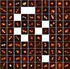 |
Fig. 1 FIRST images of the 91 X-shaped galaxies selected by Cheung (2007) with available SDSS images. The color scale and the image size (ranging from 50 to 200″) have been selected to emphasize the wing structure. The 53 galaxies with well-defined wings selected for analysis are shown with a green circle (those rejected with a red circle). |
Among the 100 XRSs selected by Cheung (2007), we only considered the 91 sources covered by the SDSS, thus excluding nine objects, namely XRS 14, 15, 23, 37, 43, 46, 54, 57, and 87. The FIRST images of the 91 objects we considered are shown in Fig. 1.
The presence of distortions and/or radio structures, in addition to the classical main double-lobed morphology, are often present in extended radio sources, including the X-shaped morphology, but they also show S-shaped structures, a “bottle-neck”, and overall bendings and asymmetries of the radio lobes. The initial Cheung sample is based on the presence of an X-shaped radio morphology. However, classifying the morphology of radio-galaxies into the various subclasses relies on subjective choices, further complicated by projection effects. In addition, the depth and resolution of the FIRST images does not always allow us to properly inspect the structure of a given source. Indeed an object-by-object analysis shows that, in some cases, such a structure is not sufficiently well defined. We therefore prefer to filter the objects, preserving only those with the clearest X-shaped morphology. This is also necessary to restrict the analysis to the objects in which the wings are sufficiently well developed and defined to allow us to derive their geometrical parameters (one of the main points of our study) with a good degree of accuracy. Operatively we graded all sources by using a score ranging from one (the best XRSs examples) to four (the less convincing ones). The grades are based on various morphological aspects, the most important of which is that the lateral extension in the radio images should not originate from the lobe end; in this case, rather common in the sample (including, for example, XRS 01, 10, 21, and 40), we consider such objects as Z- or C-shaped sources. Furthermore, the lateral extensions of bona fide XRSs must be located on the opposite sides of the main radio axis. In several sources, however, the morphology is very complex and it is difficult to recognize even the main lobes (such, as, for example, XRS 02, 39, and 55). In a many objects, the radio structure suggests an X-shaped morphology, but the FIRST resolution is insufficient to explore in detail their structures (e.g., XRS 74 and 95); these objects are not included in the clean XRSs sample. The grades were associated with all 91 sources independently by the three authors, and we only kept the 53 galaxies in the sample where the average grade was ≤2 (see Table 1). While we were completing our analysis, Roberts et al. (2015) published an atlas of radio maps of 52 sources from the Cheung sample (44 in common with our subsample) mostly obtained at 1.4 GHz with a resolution of ∼1″. These images allow us to test our initial classification based on the lower resolution FIRST images, in particular for the objects with the least extended radio emission. Although in several of the Roberts et al. images the low brightness extensions are resolved out, they often improve our ability to recognize XRSs. The result of this comparison is reported in Table 1. In two sources the XRS classification based on the high-resolution images (and on the same criteria listed above) is less secure; the opposite outcome occurs for five objects. We note that, with only one exception, these are all sources with scores of 2.00 or 2.33, i.e., borderline objects. Since high resolution images are available for less than half the sample, we prefer to maintain the classification based on the FIRST images for the following analysis; nonetheless we will discuss the effects of including/excluding the objects of uncertain nature.
Average morphological score of the 91 radio-sources.
We then proceeded at the identification of the host of the XRSs in the SDSS images. The host was sought close to the midpoint of the line joining the peaks of the two main radio lobes. In most cases the association is straightforward. Nonetheless, in XRS 05, the apparent host is significantly offset from the radio axis, in three cases (XRS 25, 60, and 75) there is more than one plausible optical identification (we then tentatively adopt the closest to the center of the radio sources), while for XRS 36, no optical emission is seen close to the center of the radio source (see Fig. 2).
3. Measurement of the optical position angle
We estimated the optical position angle, θopt, of the XRS’s host by using the SDSS images. In most cases, the i band image was used because of its higher signal-to-noise ratio (S/N). Only for XRS 06 did we instead use the r-band image because its i-band image is strongly contaminated by an emission line feature.
The classical approach to estimate θopt is based on the fitting of elliptical isophotes to the optical images. We followed this method by using the IRAF task ellipse (Jedrzejewski 1987). However, in the case of the XRS’s hosts, this is successful for only a minority of objects, mostly because of their rather small angular size. As a consequence, we prefer to adopt a different strategy, free from any prior assumption on the galaxy’s shape, which is more robust and effective for small objects. For each galaxy, we projected its optical image onto an axis whose orientation varies from 0◦ to 180◦. The orientation of the galaxy’s major axis is defined as the angle at which the width of the projected profile (measured as the standard deviation of the one-dimensional image) reaches its maximum. In Fig. 3 we show two examples.
To estimate the error on the optical PA we used the bootstrap technique. To each original image we added a random noise image (whose amplitude is defined from a blank area close to the region of interest) and re-estimated the PA. This procedure was repeated 1000 times. The PA error is defined as the range that includes 95% of the resulting values, corresponding approximatively to a 2σ level. The distribution of PA derived for one galaxy is shown in Fig. 3, right panel. By using the same method, we estimated the central value (and the error) of the host’s size (defined as 2.35 times the standard deviation of the projected profile), its axial ratio, and the difference between the major and minor axis.
In nine galaxies the optical source has an insufficient S/N to return a useful measurement of its geometrical parameters and, as a result, the error on their optical PA exceeds 45◦. These sources are marked as “faint” (or “undetected”) in Table 2.
For a successful measurement of the optical position angle we adopted the following criteria: 1) the axial ratio of the source must be higher than 1.05 and 2) the difference between the width along the minor and major axis must be greater than 0.̋15. In both cases, the requirements must be met at least at the 2 σ level. The results are tabulated in Table 2. We have a positive outcome for 22 galaxies, for which we report the optical PA and its error in Table 3. We note that i) all galaxies that meet the first requirement also meet the second, indicating that the check based on the axial ratio is actually more restrictive and ii) by adopting lower thresholds (1.03 for the axial ratio and 0.̋1 for the axis difference) no additional source would be found. We now consider the XRSs with uncertain optical counterparts, as discussed in Sect. 2, namely XRS 25, 60, and 75. Because it is impossible to measure θopt for any of them, they do not represent an issue for the analysis from this point of view.
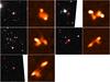 |
Fig. 2 The five cases of uncertain or unsuccessful optical counterpart identifications. The circle(s) indicate the location of the possible host(s) in both the optical SDSS (left) and radio FIRST (right) images. |
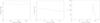 |
Fig. 3 Left and central panels: galaxy’s size (defined as 2.35 times the standard deviation in arcseconds of the projected profile) at varying angle of the projection axis for objects XRS 05 and XRS 07. Right panel: distribution of optical position angle, derived for XRS 07 from the bootstrap technique (see text for details). |
Parameters for the 53 X-shaped RG with SDSS images.
The method adopted to measure θopt, although efficient and robust, has the drawback of providing measurements of the galaxy’s axis and ellipticity that are not straightforward to compare with previous analysis. Consequently, we present two tests to better understand our results.
We produced images of a gaussian source with a FWHM of 1″ and applied the same procedure used for the galaxies and obtained a size of  , significantly smaller than the input width. This is understandable given that the one-dimensional projection returns a more concentrated profile with respect to the radial profile than is normally used to measure the FWHM.
We also test model galaxies at various distances. More specifically, we produce images of elliptical galaxies following a De Vaucouleur’s law, with an effective radius of 4.6 kpc, the value measured by Donzelli et al. (2007) for 3C radio-galaxies. The model is then convolved with a gaussian with FWHM of  to simulate the effects of seeing. For a galaxy at z = 0.4 (as we will see, typical of our sample) and with an ellipticity of 0.2, the galaxy’s size is ∼
 , the difference between the two axis is
  , and the axial ratio is 1.11. Such a galaxy, provided that the signal-to-noise ratio of its image is sufficient, would correspond to a positive outcome. However, for an ellipticity of 0.1, the axial ratio is only 1.06 and the axis difference is
  ; the analysis of such a source would not return an optical position angle.
4. Optical versus radio-wings axis
Having measured the optical PA, we can proceed to estimate the radio PA of the wings for the 22 XRSs. For each one, we produced a polar diagram of the radio emission by using the host galaxy as origin. Contours of the FIRST images in polar coordinates for three representative XRSs are shown in Fig. 5. While the main peaks in the polar diagrams are associated with the primary lobes and hot spots, the secondary ones are located at the PA of the radio wings. In particular we show XRS 03, where the faint SW wing is well visible as a secondary peak in the polar diagram, the single winged XRS 61, and the extended and diffuse wings of XRS 76, which produces well defined linear features in this figure. The resulting values of wing PA, defined as the orientation of the wings where they reach the local 3σ level, are tabulated in Table 3. We note that in several cases, only one of the wings is visible.
As a result of the complex structure of the radio wings, which often show sub-structures and bendings, the wings’ PA vary depending on the adopted reference surface-brightness level. Thus an estimate of the error in their axis can only obtained by visual inspection. For each XRS we explored both the polar diagram and the FIRST map to define the acceptable range of wing orientations. Operatively, rather than defining a specific error to each individual wing, we divided them into two groups to which we assigned PA errors of 10◦ and 20◦, respectively. In Fig. 6 we show graphically two examples of errors on the radio PA measurements. However, as we show below, the precise value of the radio PA error does not have a significant effect on our results concerning the relationship between optical and radio structures.
Optical and radio position (in degrees, from north to east) of X-shaped radio-galaxies with marks ≤2 and for which is is possible to measure the optical PA.
In Fig. 4 we show side by side, the optical and radio image of the 22 XRSs for which the optical position angle can be measured.
The difference between the optical and radio axis are given in Table 3 and shown as a histogram in Fig. 7. When both radio-wings are detected we adopted the average offset. There is a clear preference in favor of values higher than 40◦, with only one object (namely XRS 11) below this value. The probability, obtained with the Kolmogoroff-Smirnov test, that this is compatible with a uniform distribution is P = 0.9 × 10⁻⁴.
Interestingly, Battye & Browne (2009) found that red elliptical galaxies of relatively low radio-loudness show a highly significant alignment between the radio major axis and the optical minor axis; however this effect is far less pronounced with respect to what we found for the radio wings, and they interpreted this as due to a bias for the spin axis of the central engine being aligned with the minor axis of the host.
At this stage we consider the effects of the inclusion/exclusion of the sources suggested by the inspection of the higher resolution radio images from Roberts et al. (2015). The two sources for which an X-shape morphology is less secure are XRS 05 and 12, but no measurement of the optical PA was possible in these objects. The objects that might instead be included are XRS 27, 32, 62, 69, and 92). We perform the same analysis as for the other XRSs and in only 2 (XRS 27 and 92) we could measure the optical PA (154◦ and 135◦, respectively). Since the radio-optical PA differences are 44◦ and 75◦1, respectively, the inclusion of these two sources would strengthen the statistical significance of our results.
To account for the measurement errors in both the optical and radio PA, we again used the bootstrap method. We extracted 10 000 times 22 pairs of PA values with a normal distribution centered on the best value and with a width given by the PA error. We then estimated the radio-optical offsets. The histogram of the resulting probability is shown in Fig. 8. The average value is P = 7 × 10⁻⁴. To account for the uncertainties in our estimates of the error in the wings PA, we repeated the analysis doubling all values, finding that the average probability increases only to P = 5 × 10⁻³.
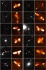 |
Fig. 4 SDSS (left) and FIRST (right) images of the 22 X-shaped galaxies for which the optical position angle can be measured. In the SDSS images the host is shown by two red ticks, each of them 16″ long and separated by 8″. The tick(s) overplotted onto the FIRST image indicated the PA of the radio wing(s), while the blue cross is at the location of the optical counterpart. |
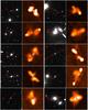 |
Fig. 4 continued. |
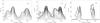 |
Fig. 5 Radio contours of the FIRST images in polar coordinates for 3 representative XRSs. The contours start at three times the local rms of the images, i.e., usually at ∼0.5 mJy/beam. |
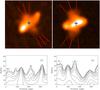 |
Fig. 6 Top panels: FIRST images of two XRSs (XRS 50 and XRS 94, on the left and right side, respectively) graphically showing the errors in the measurement of the wings PA. The solid red line indicates the central value, the dashed ones differ by the estimated errors, i.e., 20°, except for the SW wing of XRS 50, where the error is 10°. Bottom panels: polar diagrams with the wings PA values and errors indicated. |
We conclude that a highly significant connection exists between the optical and the radio-wings axis, with the wings preferentially aligned with the host’s minor axis. The same result has been obtained by Capetti et al. (2002) from the study of a sample of nine XRSs selected from the literature. Thanks to the larger size of the sample considered here, the statistical significance is strongly improved. Since the XRSs samples in these two studies do not have objects in common, the overall probability that XRS wings are randomly oriented with respect to their hosts is even lower than the ∼10-3 probability quoted here. Capetti et al. (2002) also find that wings form in galaxies with a larger ellipticity with respect to a reference sample of non-winged FR II radio-galaxies. We cannot confirm the overall validity of this finding since the 22 XRSs for which we can measure the optical axis are at a much larger distance than those studied by Capetti et al., with a median redshift of the two samples being 0.31 and 0.085, respectively. Generally, the larger distance compromises an accurate measurement of the ellipticity of XRSs hosts. However, if we focus on the four XRSs with z< 0.1 (namely, XRS 44, XRS 49, XRS 76, and XRS 83), they have an ellipticity in the range 0.21−0.36, which is similar to the XRSs considered by Capetti et al. and larger than the median ellipticity of FR II radio-galaxies (∼0.13).
The relationship between the optical axis and wings orientation suggests the existence of causal connection between the presence of radio wings (and thus the origin of XRSs) and the properties of their host. Our results strengthen the interpretation proposed by Capetti et al. that XRSs naturally form when a jet propagates in a non-spherical gas distribution. In this case, the cocoon expansion along the direction of maximum pressure gradient (the galaxy minor axis) occurs at a speed comparable to that of the advance of the jet head along the radio source main axis, producing the X-shaped morphology.
Spectral properties of the 26 X-shaped RG with SDSS/BOSS spectra.
5. Redshift and radio power of XRSs
We collected the spectroscopic redshifts for our sources from Cheung et al. (2009) and Landt et al. (2010), see Table 2. When no spectroscopic redshift is available, we adopt the photometric redshifts provided by the SDSS database, which were estimated with the kd-tree nearest neighbor (KD, Csabai et al. 2007) or the random forests (RF, Carliles et al. 2010) methods. Only in three cases was no redshift estimate available.
The comparison between the spectroscopic and photometric redshifts for the 26 XRSs where these two quantities are available indicates that the average relative differences are | zspec − zphot | /zspec = 0.13 for both the KD and RF methods. When only the two photo-z estimates are available they are, with only two exceptions, consistent with each other within the errors. This indicates that the redshift estimates (and the corresponding radio luminosities) are generally robust. In Fig. 6 we present the radio luminosity histograms of XRSs, having taken the 1.4 GHz from the FIRST catalog as published by Cheung et al. (2009). In the two panels the luminosities have been estimated, when no spectroscopic redshift is measured, by adopting the KD and RF values, respectively. The red histograms represent the fraction of objects with spectroscopic redshifts. The radio luminosity distribution spans the range L ∼ 1032−1034 erg s-1 Hz-1 at 1.4 GHz, regardless of the photo-z adopted.
XRSs extend by a factor of 10 below the least luminous FR II of the 3CR sample (Buttiglione et al. 2009), but this effect has already been noted by Kozieł-Wierzbowska & Stasińska (2011) from the analysis of FR II that was extracted from the SDSS. More interesting is the presence of a high power cut-off for XRSs. We cannot firmly conclude that this is not related to some selection bias that is due, for example, to the detectability of the wings and of the hosts in higher redshift/power objects; indeed, the objects in which we could measure the optical PA have a median redshift of 0.30, against 0.43 for the sources where this estimate was unsuccessful; alternatively this result can be interpreted in the framework of the lateral cocoon expansion model presented above. In fact, high luminosity radio galaxies that are associated with jets of greater power are less affected by the properties of the surrounding medium. They might escape the region where the cocoon expansion in influenced by the asymmetric host before the lateral wings can develop.
6. Spectral analysis
The aim of this section is to derive information on the spectroscopic properties of XRSs from the point of view of their stellar population and emission lines. This analysis can falsify the proposed model that poses that XRSs are “normal” FR II whose radio morphology is only caused by the jet propagation in an asymmetric ISM. In fact, no differences are expected between the XRS’s properties and those of non-winged FR II. However, we note that the competing model based on jet re-orientation (due, e.g., to a galaxies merger) does not require an enhanced star-formation activity to be observed in XRSs, since this is expected only when one of the coalescing galaxies is gas rich; no effect on the stellar population is expected from a “dry” merger. Furthermore, there might be a substantial temporal gap between the various phases of the merger event, i.e., the black hole coalescence and reorientation, the phase of high star formation, and the onset of the AGN activity (e.g., Blecha et al. 2011).
We collected the available 28 SDSS spectra for the selected sub-sample of 53 XRSs. For two XRSs (namely, XRS 48 and 73) we do not proceed with this analysis since they are quasars with no visible starlight. The resulting list of 26 objects is presented in Table 4. Each spectrum is modeled by using the Gandalf software (Sarzi et al. 2006) from which we obtain a decomposition of the stellar light into 39 templates and the measurements of their emission lines. The different emission lines were all fixed to the same velocity by using, as an initial guess, the host redshift.
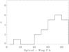 |
Fig. 7 Difference between optical and wing PA (in degrees) for the 22 XRSs for which such a comparison is possible. When two wings are present, we averaged the two values. |
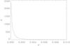 |
Fig. 8 Distribution of probability resulting from a Kolmogoroff-Smirnov test that the distribution of offsets between optical and radio-wing axis is compatible with a uniform distribution. This is obtained with the bootstrap method from 10 000 realizations that result from randomly varying both axis around the central values with an amplitude given by the measurements errors. |
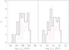 |
Fig. 9 Radio luminosity distribution of XRSs at 1.4 GHz; the luminosities are estimated, when no spectroscopic redshift is available by adopting the KD and RF photometric redshifts, in the left and right panel, respectively. The red histograms represent the fraction of objects with spectroscopic redshifts. |
6.1. Emission line properties
The emission line measurements of the 26s XRSs are used to build the diagnostic diagram to derive a spectroscopic classification. This is obtained by comparing the ratio of the intensity between [O III] and Hβ with those of the [N II], [S II], and [O I] line against Hα, following the analysis presented by Kewley et al. (2006). In eight cases the Hβ line (and often also the [O III] line) is not detected; furthermore, the Hα line falls outside six SDSS spectra because of their high redshift. We are then left with 11 objects that can be located in the diagnostic diagrams (see Fig. 10). We classify a source as HEG when it falls above the dashed lines that mark the boundaries between HEGs and LEGs, as derived from the 3CR radio-galaxies (Buttiglione et al. 2010). Two objects (namely XRS 78 and 90) fall into the HEGs region in the left and right panels, while, in the LEGs region, they are only in the middle one: we consider them as HEGs (a conclusion that will be strengthened by their location in the diagram that compares line and radio luminosity, see below). We find seven HEGs and four LEGs.
Considering again the six high redshift sources with no information on the Hα line, in all cases the [O III]/Hβ is larger than eight. Since no LEG in the 3CR is found above this ratio, we consider them as HEGs.
6.2. Radio and emission line properties
We now consider the relation between emission lines and radio luminosity. In 3C radio-galaxies the two spectral types follow different correlations between L[O III] and Lr, with HEGs having larger line luminosity at given radio power. In Fig. 11 we compare emission lines and radio luminosity, color-coding the different source types. Both HEGs and LEGs among the XRSs are located close to the respective correlations defined by the 3CR RGs.
As already noticed in the 3C sample, several galaxies of uncertain spectral classification can be classified robustly based on their location in this diagram. In fact, with the sole exception of XRS 72, all unclassified sources fall very closely along the L[O III] − Lr relation defined by 3CR LEGs. With this strategy we are able to define a spectral type for all but one of the XRSs.
6.3. Stellar populations
The Gandalf software provides us also with a decomposition of the starlight among the 39 templates of varying metallicity (from solar to thrice solar) and age (up to 12 Gyr) from Bruzual & Charlot (2003). In Fig. 12 we show the result of this analysis. For each source we show the contribution of the 39 models used, formed by combining three different metallicities (Y axis) and 13 different ages (X axis). The area of the symbols show the relative contribution of each template to the XRS’s starlight.
HEGs are known to show almost invariably blue colors, an indication of recent star formation, while in LEGs, the fraction of actively star-forming objects is not enhanced with respect to quiescent galaxies (Baldi & Capetti 2008; Smolčić 2009). A quantitative comparison between these results and those presented here cannot be performed since the indicators of young stars are rather different. Furthermore, the precise decomposition in the various stellar populations is rather uncertain, being affected by, e.g., the age-metallicity degeneracy. Nonetheless, a prominent young stellar population (with an age ≤3 Gyr and a fractional contribution of at least 10%) is found in eight (out of 13) HEGs and in only one (out of 12) LEGs among the XRSs.
Apparently, both the emission lines and the stellar population properties of XRSs do not differ from those of 3C FR II. This is what is expected if the appearance of the radio wings is due to the hosts asymmetries.
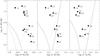 |
Fig. 10 Spectroscopic diagnostic diagrams: (left) [O III]/Hβ vs. [N II]/Hα ratios, (center) [O III]/Hβ vs. [S II]/Hα ratio, (right) [O III]/Hβ vs. [O I]/Hα. The curves divide AGN (above the solid curved line) from star-forming galaxies. In the left panel, between the long-dashed and solid curve are the composite galaxies (Kewley et al. 2006). In the middle and right panels, the straight solid line divides Seyferts (upper left region) from LINERs (right region). The dashed lines mark the approximate boundaries between HEGs and LEGs derived from the 3CR radio-galaxies in each diagram, from Buttiglione et al. (2010), Fig. 7. |
7. Summary and conclusions
The aim of this paper is to explore the properties of XRSs, from the point of view of the geometrical relationship between radio and optical structures, of their emission lines, and of their stellar population. Starting with a sample of XRSs identified in the FIRST survey and covered by the SDSS, we restrict our analysis to the 53 objects with the clearest X-shaped morphology. The identification of the host of the XRSs in the SDSS images is, in most cases, straightforward since we found a single optical source located close to the midpoint of the line that joins the peaks of the two main radio lobes. Only in five sources is the identification not secure, because we either have more than one plausible association or no optical source is found at the center of the radio source.
Spectroscopic redshifts are available for 35 sources and for all others (except three) there are photometric redshift measurements provided by the SDSS database. The median redshift is z = 0.31. At this distance, the typical core size of RG’s hosts covers only 1″. Indeed, most of the XRS’s hosts are rather compact sources in the SDSS images: the classical approach for estimating the position angle of the hosts major axis, based on fitting elliptical isophotes to the optical images, cannot generally be used.
Consequently, we adopt a different strategy: for each galaxy, we projected its optical image onto an axis. The orientation of the galaxy’s major axis is defined as the angle at which the width of the projected profile reaches its maximum. With this method, we also derive the host’s size and axial ratio. The bootstrap technique was used to estimate the errors of these quantities. While some galaxies are too faint, too compact, or not sufficiently elongated, we obtain a robust measurement of the PA of the major axis for 22 galaxies.
We find that the radio-wing axis of all (but one) of the XRSs form an angle larger than 40◦ with the optical major axis, with a probability that this is compatible with a uniform distribution of only P = 0.9 × 10⁻⁴. A highly significant connection between the optical and the radio-wing axis emerges, with the wings preferentially aligned with the host’s minor axis, This confirms the previous findings but, because of the larger size of the sample studied, with a strongly improved statistical significance. We also confirm that wings develop in highly elliptical galaxies, although this conclusion can only be obtained from the study of the four nearest XRSs.
The relationship between the optical axis and wing orientation indicate that the formation of the XRSs is intimately related to the host’s geometry. These results strengthen the interpretation that the X-shaped morphology in radio-sources has an hydro-dynamical origin, rather than being the result of a jet-reorientation following a black hole coalescence. In particular XRSs naturally form when a jet propagates in a non-spherical gas distribution: the rapid cocoon expansion along the direction of the host’s minor axis produces the X-shaped morphology.
In this framework, it is possible to further progress in our understanding of the origin of XRSs along two lines. Firstly, we used the optical imaging data obtained from the SDSS. This survey provides us with a homogeneous dataset, but of limited depth; a targeted optical survey can lead to a higher number of radio galaxies for which it is possible to measure the geometrical parameters. Finally, the planned JVLA surveys will produce deeper and higher resolution images, enabling an even larger sample of bona-fide XRSs to be built.
We have also performed a study of the properties of the emission lines (and their connection with the spectroscopic types and radio luminosity) as well as of their stellar population. This analysis can falsify the proposed model that poses that XRSs are “normal” FR II, whose radio morphology is only caused by an asymmetric ISM. In fact, in this case, no differences are expected between the XRS’s properties and those of non-winged FR II. Conversely, any anomaly of XRSs with respect to non-winged FR II may indicate that they are the result of a specific evolutionary path, such as, one that involves the occurrence of a merger. This is one of the requirements of the jet re-orientation scenario, an alternative to the hydro-dynamical model we propose. A proper classification into the various spectroscopic classes is essential for a proper comparison with non-winged radio galaxies. We do not find any difference between the properties of XRSs and the general FR II population.
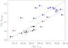 |
Fig. 11 Comparison of the luminosity of the [O III] line and the radio power at 1.4 GHz (in erg s-1 and erg s-1 Hz-1 units, respectively). The XRSs are color-coded based on their classification: blue = HEG, red = LEG, black = unclassified. |
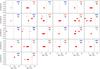 |
Fig. 12 Decomposition of the starlight emission in various templates of stellar populations obtained with Gandalf. For each source we show the contribution of the 39 models used, formed by combining set with three different metalicity (Y axis) and 13 different ages (X axis). The area of the symbols show the relative contribution of each template. The dashed vertical line marks the age of the Universe at the redshift of each source. |
For J1606+0000 we used the Hodges-Kluck et al. (2010) radio images.
References
- Baldi, R. D., & Capetti, A. 2008, A&A, 489, 989 [NASA ADS] [CrossRef] [EDP Sciences] [Google Scholar]
- Battye, R. A., & Browne, I. W. A. 2009, MNRAS, 399, 1888 [NASA ADS] [CrossRef] [Google Scholar]
- Blecha, L., Cox, T. J., Loeb, A., & Hernquist, L. 2011, MNRAS, 412, 2154 [NASA ADS] [CrossRef] [Google Scholar]
- Bruzual, G., & Charlot, S. 2003, MNRAS, 344, 1000 [NASA ADS] [CrossRef] [Google Scholar]
- Buttiglione, S., Capetti, A., Celotti, A., et al. 2009, A&A, 495, 1033 [NASA ADS] [CrossRef] [EDP Sciences] [Google Scholar]
- Buttiglione, S., Capetti, A., Celotti, A., et al. 2010, A&A, 509, A6 [NASA ADS] [CrossRef] [EDP Sciences] [Google Scholar]
- Capetti, A., Zamfir, S., Rossi, P., et al. 2002, A&A, 394, 39 [Google Scholar]
- Carliles, S., Budavári, T., Heinis, S., Priebe, C., & Szalay, A. S. 2010, ApJ, 712, 511 [NASA ADS] [CrossRef] [Google Scholar]
- Cheung, C. C. 2007, AJ, 133, 2097 [NASA ADS] [CrossRef] [Google Scholar]
- Cheung, C. C., Healey, S. E., Landt, H., Verdoes Kleijn, G., & Jordán, A. 2009, ApJS, 181, 548 [NASA ADS] [CrossRef] [Google Scholar]
- Csabai, I., Dobos, L., Trencséni, M., et al. 2007, Astron. Nachr., 328, 852 [NASA ADS] [CrossRef] [Google Scholar]
- Dennett-Thorpe, J., Scheuer, P. A. G., Laing, R. A., et al. 2002, MNRAS, 330, 609 [NASA ADS] [CrossRef] [Google Scholar]
- Donzelli, C. J., Chiaberge, M., Macchetto, F. D., et al. 2007, ApJ, 667, 780 [NASA ADS] [CrossRef] [Google Scholar]
- Ekers, R. D., Fanti, R., Lari, C., & Parma, P. 1978, Nature, 276, 588 [NASA ADS] [CrossRef] [Google Scholar]
- Fanaroff, B. L., & Riley, J. M. 1974, MNRAS, 167, 31 [NASA ADS] [CrossRef] [Google Scholar]
- Gopal-Krishna, Biermann, P. L., Gergely, L. Á., & Wiita, P. J. 2012, RA&A, 12, 127 [Google Scholar]
- Hodges-Kluck, E. J., Reynolds, C. S., Cheung, C. C., & Miller, M. C. 2010, ApJ, 710, 1205 [NASA ADS] [CrossRef] [Google Scholar]
- Jedrzejewski, R. I. 1987, MNRAS, 226, 747 [Google Scholar]
- Kewley, L. J., Groves, B., Kauffmann, G., & Heckman, T. 2006, MNRAS, 372, 961 [NASA ADS] [CrossRef] [Google Scholar]
- Klein, U., Mack, K.-H., Gregorini, L., & Parma, P. 1995, A&A, 303, 427 [NASA ADS] [Google Scholar]
- Kozieł-Wierzbowska, D., & Stasińska, G. 2011, MNRAS, 415, 1013 [NASA ADS] [CrossRef] [Google Scholar]
- Landt, H., Cheung, C. C., & Healey, S. E. 2010, MNRAS, 408, 1103 [NASA ADS] [CrossRef] [Google Scholar]
- Leahy, J. P., & Williams, A. G. 1984, MNRAS, 210, 929 [NASA ADS] [CrossRef] [Google Scholar]
- Merritt, D., & Ekers, R. D. 2002, Science, 297, 1310 [NASA ADS] [CrossRef] [PubMed] [Google Scholar]
- Mezcua, M., Lobanov, A. P., Chavushyan, V. H., & León-Tavares, J. 2011, A&A, 527, A38 [NASA ADS] [CrossRef] [EDP Sciences] [Google Scholar]
- Mezcua, M., Chavushyan, V. H., Lobanov, A. P., & León-Tavares, J. 2012, A&A, 544, A36 [NASA ADS] [CrossRef] [EDP Sciences] [Google Scholar]
- O’Dea, C. P., & Owen, F. N. 1986, ApJ, 301, 841 [NASA ADS] [CrossRef] [Google Scholar]
- Rees, M. J. 1978, Nature, 275, 516 [NASA ADS] [CrossRef] [Google Scholar]
- Roberts, D. H., Cohen, J. P., Lu, J., Saripalli, L., & Subrahmanyan, R. 2015, ApJS, 220, 7 [NASA ADS] [CrossRef] [Google Scholar]
- Saripalli, L., & Subrahmanyan, R. 2009, ApJ, 695, 156 [NASA ADS] [CrossRef] [Google Scholar]
- Sarzi, M., Falcón-Barroso, J., Davies, R. L., et al. 2006, MNRAS, 366, 1151 [NASA ADS] [CrossRef] [Google Scholar]
- Smolčić, V. 2009, ApJ, 699, L43 [NASA ADS] [CrossRef] [Google Scholar]
- Wirth, A., Smarr, L., & Gallagher, J. S. 1982, AJ, 87, 602 [NASA ADS] [CrossRef] [Google Scholar]
- Worrall, D. M., Birkinshaw, M., & Cameron, R. A. 1995, ApJ, 449, 93 [NASA ADS] [CrossRef] [Google Scholar]
All Tables
Optical and radio position (in degrees, from north to east) of X-shaped radio-galaxies with marks ≤2 and for which is is possible to measure the optical PA.
All Figures
|
Fig. 1 FIRST images of the 91 X-shaped galaxies selected by Cheung (2007) with available SDSS images. The color scale and the image size (ranging from 50 to 200″) have been selected to emphasize the wing structure. The 53 galaxies with well-defined wings selected for analysis are shown with a green circle (those rejected with a red circle). |
| In the text | |
|
Fig. 2 The five cases of uncertain or unsuccessful optical counterpart identifications. The circle(s) indicate the location of the possible host(s) in both the optical SDSS (left) and radio FIRST (right) images. |
| In the text | |
|
Fig. 3 Left and central panels: galaxy’s size (defined as 2.35 times the standard deviation in arcseconds of the projected profile) at varying angle of the projection axis for objects XRS 05 and XRS 07. Right panel: distribution of optical position angle, derived for XRS 07 from the bootstrap technique (see text for details). |
| In the text | |
|
Fig. 4 SDSS (left) and FIRST (right) images of the 22 X-shaped galaxies for which the optical position angle can be measured. In the SDSS images the host is shown by two red ticks, each of them 16″ long and separated by 8″. The tick(s) overplotted onto the FIRST image indicated the PA of the radio wing(s), while the blue cross is at the location of the optical counterpart. |
| In the text | |
|
Fig. 4 continued. |
| In the text | |
|
Fig. 5 Radio contours of the FIRST images in polar coordinates for 3 representative XRSs. The contours start at three times the local rms of the images, i.e., usually at ∼0.5 mJy/beam. |
| In the text | |
|
Fig. 6 Top panels: FIRST images of two XRSs (XRS 50 and XRS 94, on the left and right side, respectively) graphically showing the errors in the measurement of the wings PA. The solid red line indicates the central value, the dashed ones differ by the estimated errors, i.e., 20°, except for the SW wing of XRS 50, where the error is 10°. Bottom panels: polar diagrams with the wings PA values and errors indicated. |
| In the text | |
|
Fig. 7 Difference between optical and wing PA (in degrees) for the 22 XRSs for which such a comparison is possible. When two wings are present, we averaged the two values. |
| In the text | |
|
Fig. 8 Distribution of probability resulting from a Kolmogoroff-Smirnov test that the distribution of offsets between optical and radio-wing axis is compatible with a uniform distribution. This is obtained with the bootstrap method from 10 000 realizations that result from randomly varying both axis around the central values with an amplitude given by the measurements errors. |
| In the text | |
|
Fig. 9 Radio luminosity distribution of XRSs at 1.4 GHz; the luminosities are estimated, when no spectroscopic redshift is available by adopting the KD and RF photometric redshifts, in the left and right panel, respectively. The red histograms represent the fraction of objects with spectroscopic redshifts. |
| In the text | |
|
Fig. 10 Spectroscopic diagnostic diagrams: (left) [O III]/Hβ vs. [N II]/Hα ratios, (center) [O III]/Hβ vs. [S II]/Hα ratio, (right) [O III]/Hβ vs. [O I]/Hα. The curves divide AGN (above the solid curved line) from star-forming galaxies. In the left panel, between the long-dashed and solid curve are the composite galaxies (Kewley et al. 2006). In the middle and right panels, the straight solid line divides Seyferts (upper left region) from LINERs (right region). The dashed lines mark the approximate boundaries between HEGs and LEGs derived from the 3CR radio-galaxies in each diagram, from Buttiglione et al. (2010), Fig. 7. |
| In the text | |
|
Fig. 11 Comparison of the luminosity of the [O III] line and the radio power at 1.4 GHz (in erg s-1 and erg s-1 Hz-1 units, respectively). The XRSs are color-coded based on their classification: blue = HEG, red = LEG, black = unclassified. |
| In the text | |
|
Fig. 12 Decomposition of the starlight emission in various templates of stellar populations obtained with Gandalf. For each source we show the contribution of the 39 models used, formed by combining set with three different metalicity (Y axis) and 13 different ages (X axis). The area of the symbols show the relative contribution of each template. The dashed vertical line marks the age of the Universe at the redshift of each source. |
| In the text | |
Current usage metrics show cumulative count of Article Views (full-text article views including HTML views, PDF and ePub downloads, according to the available data) and Abstracts Views on Vision4Press platform.
Data correspond to usage on the plateform after 2015. The current usage metrics is available 48-96 hours after online publication and is updated daily on week days.
Initial download of the metrics may take a while.