| Issue |
A&A
Volume 587, March 2016
|
|
|---|---|---|
| Article Number | A33 | |
| Number of page(s) | 8 | |
| Section | The Sun | |
| DOI | https://doi.org/10.1051/0004-6361/201527039 | |
| Published online | 12 February 2016 | |
Variation of the Mn I 539.4 nm line with the solar cycle
1 Max-Planck-Institut für Sonnensystemforschung, Justus-von-Liebig-Weg 3, 37077 Göttingen, Germany
e-mail: This email address is being protected from spambots. You need JavaScript enabled to view it.
2 School of Space Research, Kyung Hee University, Yougin, 446-701 Gyeonggi, Korea
3 National Solar Observatory, 950 North Cherry Avenue, Tucson, AZ 85718, USA
4 Astronomical Observatory, Volgina 7, 11160 Belgrade 74, Serbia
Received: 22 July 2015
Accepted: 27 October 2015
Abstract
Context. As a part of the long-term program at Kitt Peak National Observatory (KPNO), the Mn i 539.4 nm line has been observed for nearly three solar cycles using the McMath telescope and the 13.5 m spectrograph in double-pass mode. These full-disk spectrophotometric observations revealed an unusually strong change of this line’s parameters over the solar cycle.
Aims. Optical pumping by the Mg II k line was originally proposed to explain these variations. More recent studies have proposed that this is not required and that the magnetic variability (i.e., the changes in solar atmospheric structure due to faculae) might explain these changes. Magnetic variability is also the mechanism that drives the changes in total solar irradiance variations (TSI). With this work we investigate this proposition quantitatively by using the same model that was earlier successfully employed to reconstruct the irradiance.
Methods. We reconstructed the changes in the line parameters using the model SATIRE-S, which takes only variations of the daily surface distribution of the magnetic field into account. We applied exactly the same model atmospheres and value of the free parameter as were used in previous solar irradiance reconstructions to now model the variation in the Mn i 539.4 nm line profile and in neighboring Fe i lines. We compared the results of the theoretical model with KPNO observations.
Results. The changes in the Mn i 539.4 nm line and a neighbouring Fe i 539.52 nm line over approximately three solar cycles are reproduced well by the model without additionally tweaking the model parameters, if changes made to the instrument setup are taken into account. The model slightly overestimates the change for the strong Fe i 539.32 nm line.
Conclusions. Our result confirms that optical pumping of the Mn ii 539.4 nm line by Mg II k is not the main cause of its solar cycle change. It also provides independent confirmation of solar irradiance models which are based on the assumption that irradiance variations are caused by the evolution of the solar surface magnetic flux. The result obtained here also supports the spectral irradiance variations computed by these models.
Key words: Sun: activity / Sun: photosphere
© ESO, 2016
1. Introduction
Solar irradiance varies on timescales of minutes to decades. For variations on timescales extending from a day to the length of the solar cycle, different causes have been proposed: changes of the internal thermal structure of the Sun, changes of subsurface fields, or changes of the field at the surface. The third explanation has found considerable support (Solanki et al. 2005, 2013; Domingo et al. 2009).
In particular, the Spectral And Total Irradiance REconstruction for the satellite era (SATIRE-S) has been successfully used to describe the variability in the changes of total irradiance during the past three cycles. At least 92% of the total solar irradiance (TSI) variability can be assigned to changes in the magnetic field distribution at the solar surface (Krivova et al. 2003, 2011; Wenzler et al. 2005, 2006; Ball et al. 2012; Yeo et al. 2014a). However, since in its present form the SATIRE-S model contains a free parameter, these conclusions may not be entirely compelling. It is therefore important to reproduce spectral features as well. This has been done for the Variability of IRradiance & Gravity Oscillations (VIRGO; Fröhlich et al. 1995) color channels by Krivova et al. (2003), UV irradiance (Krivova et al. 2006, 2009; Yeo et al. 2014a), and for spectral irradiance over a broad wavelength range on solar rotation timescales (Unruh et al. 2008).
The recent spectral data from the Spectral Irradiance Monitor (SIM) on SORCE over the declining phase of cycle 23 (cf. Harder et al. 2009), however, showed solar cycle trends that are significantly different from those expected both from earlier measurements and from models (Ermolli et al. 2013; Ball et al. 2012; Yeo et al. 2014a). In particular, irradiance in the visible between 400 and 700 nm was found to increase with the decrease of the TSI. In this paper, we use the SATIRE-S model to describe the solar cycle variability of Mn i 539.47 nm and two neighbouring neutral iron lines, which sets additional constraints on the model. Modeling the solar cycle variation of spectral lines is of particular importance since spectral lines are estimated to contribute more than 50−90% of the TSI variations over the solar cycle (Mitchell & Livingston 1991; Unruh et al. 1999). Moreover, some studies have even suggested that the solar irradiance variability in the UV, violet, blue, and green spectral domains is fully controlled by the Fraunhofer lines (Shapiro et al. 2015).
The Mn i 539.47 nm line is interesting for several reasons. The hyperfine broadening, due to the interaction of the electronic shell with the nuclear spin, makes it relatively insensitive to nonthermal motions in the photosphere (Elste & Teske 1978; Elste 1986). This was recently demonstrated by Vitas et al. (2009) with 3D magnetohydrodynamic (MHD) simulations. They showed that the Mn i 539.47 nm line is not smeared by convective motions, in contrast to the neighboring narrow Fe i 539.52 nm line, which always becomes weaker as a result of the smearing. The Mn i line, on the other hand, becomes stronger in sunspots and weaker in plages and the network, as observed by Vince et al. (2005a,b) and Malanushenko et al. (2004). This means that although the Mn i line is formed in the photosphere (Gurtovenko & Kostyk 1989; Vitas 2005), the “Sun-as-a-star” observations (Livingston & Wallace 1987; Livingston 1992) of this line exhibit a significant cycle dependence that is not typical for other photospheric lines recorded in parallel. A time-series analysis shows that even variations on the solar rotation timescale can be found around the solar activity maximum (Danilovic et al. 2005). One explanation of this chromospheric-like behavior was earlier proposed by Doyle et al. (2001). They found that optical pumping by Mg ii k might be the reason for this Mn line to mimic the change seen in Mg ii k. However, the analysis of Vitas & Vince (2007) proved that the Mn i 539.47 nm line is insensitive to the photons emitted in the cores of Mg ii h and k.
Danilovic & Vince (2005) showed that extended the modeling of the “Sun-as-a-Star” spectra of Mn i 539.47 nm could explain the change observed over a short period of solar cycle 23. Later, Vitas et al. (2009) demonstrated the change in the Mn i line in magnetic flux concentrations in one MHD snapshot, but they did not model the “Sun-as-a-Star” spectra. In this paper we model the Mn i cycle change over the full period of 1978−2009 that was covered by Livingston’s “Sun-as-a-Star” monitoring program1 (Livingston et al. 2010). In addition, we analyze the behavior of the two neighboring Fe i lines that were observed in the same spectral channel.
The structure of the paper is as follows: observations and modeling technique are described in Sect. 2. The disk-averaged line synthesis is treated in Sect. 2.3. The calculated center-to-limb variations of the line profiles are given in Sect. 3.1. Results for different observational phases (before and after 1992) and for three solar cycles are discussed in Sect. 3.3. Concluding remarks are given in Sect. 4.
2. Observational data and modeling technique
2.1. Data
The observational data modeled here were obtained with the 13.5 m scanning spectrometer set in double-pass mode and mounted on the Kitt Peak McMath telescope (Brault et al. 1971). We describe the observations in some detail since no comprehensive description exists in the literature.
The sunlight is delivered to the spectrograph without any prefocusing. There a 0.5 × 10 mm entrance slit forms a pinhole image of the Sun on the grating (camera obscura principle). This specific instrumental set produced the disk-integrated or “Sun-as-a-star” spectrum.
The 2 Å wide spectral range around the Mn i 539.47 nm line was observed in fifth order of the grating, which yielded a spectral resolution of around 106 000. Line intensities and equivalent widths were automatically extracted using the data reduction program developed by J. Brault at Kitt Peak (Brault et al. 1971). For the continuum normalization the data point at 539.491 nm was used because the comparison with the Kitt Peak spectral atlas of Wallace et al. (2007) showed that it is entirely free of telluric blends, whereas most other (pseudo-)continuum wavelengths are affected. The intensity values at this wavelength were normalized to unity. This might be slightly too high, as a comparison with spectra acquired with the Fourier Transform Spectrometer (FTS) reveals (Fig. 3). However, tests have shown that any small error introduced by this normalization does not affect the results in a significant way. A quadratic fit to the cores of each of the lines was made, and the line central depth was defined as the difference between the minimum of the fit and the normalized continuum value. The equivalent width was calculated within given wavelength ranges (shown below in Fig. 3).
A first set of observations with an unchanged setup was taken from 1979 to 1992, with recordings being made a few times each month. In 1992 a new larger grating with dimensions 42 × 32 cm2 was installed, compared with 25 × 15 cm2 for the grating mounted before 1992. This instrumental change had a measurable effect on the data. Before the change, part of the solar limb fell outside the grating, whereas with the new grating, the full solar disk was sampled. This introduced a jump in the measured equivalent width (EW) and central depth (CD) of lines obtained before and after 1992. After mounting, an experimental period with the new grating lasted until 1996, when the system was fixed and observations were performed regularly again. However, constant realignment of the system between 1996 and 1998 led to an increased variance in the parameters of the recorded spectral lines. As a result, we analyzed and modeled observations recorded on 465 days from January 1979 to September 1992 and on 463 days in the period from September 1998 to October 2009. Between September 1992 and September 1998, observations were obtained on 45 days. These were not taken into account in the work described here because of the varying settings.
2.2. SATIRE-S model
The SATIRE model described by Fligge et al. (2000) and Krivova et al. (2003) assumes that the change in solar irradiance can be explained by the evolution of the solar surface magnetic field. The model categorizes all solar surface features into four groups based on their brightness and magnetic flux density. The surface area with a brightness below a given threshold is identified as the area covered by sunspots. These are further partitioned into umbrae and penumbrae, depending on the brightness level. Facular regions are classified as areas that have a magnetic flux density above a threshold, but do not belong to sunspots or pores. The areas that do not fulfil any of these criteria are classified as quiet-Sun areas. To identify the features in the period from 1978 to 2003, we used full-disk magnetograms and continuum images recorded with the 512 channel magnetograph and the spectromagnetograph, mounted on the Kitt Peak Vacuum Tower Telescope. Magnetograms obtained with MDI/SOHO were used for the later period. A detailed description of data calibration is given in Wenzler et al. (2004, 2006) and Ball et al. (2012).
Since the spatial resolution of the maps is on the order of a few arcsec, the model takes into account that magnetic elements in faculae are not fully resolved; to do this, a filling factor is introduced. It increases linearly with magnetic flux density and reaches unity at a magnetogram signal of Bsat. For B>Bsat the filling factor remains constant at 1. Bsat is the only free parameter in the SATIRE-S model. The value of Bsat = 330 G used here is the same as in Ball et al. (2012).
The stratification of physical parameters with depth was assumed to remain unchanged over the solar cycle and was represented by 1D model atmospheres (Unruh et al. 1999). The Kurucz standard solar atmosphere (Kurucz 1991, 1992) was used for the quiet Sun, and stellar models with a gravitational acceleration of log g = 4.5 m/s2 and effective temperature of 4500 K and 5400 K were used for umbrae and penumbrae, respectively. As the model atmosphere for the faculae, Unruh et al. (1999) adopted FALP from Fontenla et al. (1999), but without the chromospheric temperature increase and with a slightly smaller temperature gradient in the deeper atmospheric layers. As demonstrated in that paper, these changes provide a good agreement of synthesized and observed facular contrast in the optical range.
Line characteristics: wavelength, transition, oscillator strength, and excitation energy.
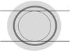 |
Fig. 1 Illustration of flux calculations for the period before 1993 when the old grating was used. The two horizontal lines delimit the part of the disk that illuminates the grating. The dashed circle corresponds to μ = μcut. |
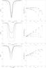 |
Fig. 2 Left-hand side: profiles of Fe i 539.32 nm, Mn i 539.47 nm, and Fe i 539.52 nm lines at the disk center, from top to bottom. The profiles are computed in the following model atmospheres: quiet Sun (dashed), faculae (dotted), penumbrae (double-dot-dashed), and umbrae (dash-dotted). FTS atlas profiles are overplotted (solid curves). Right-hand side: center-to-limb variation of the EW of the lines. Symbols distinguish between the EW resulting from different model atmospheres: quiet Sun (plus signs), faculae (asterisks), penumbrae (crosses), and umbrae (squares). Diamonds with error bars are values observed in the quiet Sun. |
2.3. Spectral line calculations
The KP spectra containing the Mn i 539.47 nm line also include two Fe i lines. These lines exhibit smaller variations over the solar cycle, allowing them to be partially used to check for changes in instrumentation etc. The main characteristics of all three lines, taken from the VALD database (Kupka et al. 1999), are given in Table 1.
The procedure of calculating disk-integrated flux in this spectral range is as follows: time-independent emergent intensities of the Mn i line and the neighboring Fe i lines are calculated in local thermal equilibrium (LTE) for each model atmosphere for various heliocentric angles using the SPINOR code (Frutiger et al. 2000). No magnetic field is introduced in the calculations. The hyperfine structure of the Mn I line is included as blends with displacements calculated using the hyperfine constants from Davis et al. (1971) and Brodzinski et al. (1987) and relative intensities of the components from Condon & Shortley (1963). Components that are closely spaced with respect to the total splitting were combined to reduce the computing effort. Emergent intensities, output from SPINOR, were then combined with the relative contributions of different features for different heliocentric angles.
Before 1993, the incomplete sampling of the solar disk by the grating had to be taken into account. Figure 1 illustrates the simple method that we applied. We assumed that the part of the image of the solar disk bounded by the two horizontal lines covers the grating, while the rest is lost due to the size of the grating. Let μcut be the cosine of the a priori unknown heliocentric angle for which the disk image fully covers the grating. Flux coming from the region shaded dark gray in the figure, for example, which corresponds to μ<μcut, is partially lost. For each of these 2-degree-wide regions we introduced coefficients proportional to the annular surfaces that lie in between the horizontal lines (shaded with short horizontal lines). The radiative flux coming from the whole annulus is multiplied by this coefficient. The coefficients are normalized such that the sum over all coefficients for every region at μ<μcut is unity. In this way, we did not specify which parts of the solar disk (heliographic latitudes and longitudes) were sampled and which were not. This treatment is appropriate since the grating received light from different parts of the solar disk during the day because the McMath telescope is fed by a heliostat. Finally, the total flux at each wavelength position was obtained by summing the fluxes multiplied by the corresponding coefficients from all heliocentric angles.
3. Results
Before computing the time series of the CD and the EW of the disk-integrated profiles of the two Fe i lines and the Mn line, we first verified that the lines were computed properly, that is, that the measured profiles of line intensity were accurately reproduced. We first computed the lines at disk center and determined their contribution functions and log gfϵ values (gf is the oscillator strength times the statistical weight of the lower level of the transition, and ϵ is the abundance). In the second step we compared their center-to-limb change (CLV) with measurements, and finally, we computed the time series of the flux computed with the SATIRE-S model.
Fitted values of oscillator strengths and macroturbulence for the disk center.
3.1. Line profiles at disk center
Employing elemental abundances from the literature and a quiet-Sun model atmosphere, we reproduced the FTS atlas profiles (Wallace et al. 2007) that were recorded in the quiet Sun at the disk center by allowing the oscillator strengths and macroturbulence broadening velocity to vary. A Gaussian profile was chosen for the macroturbulence. The best-fit values are given in Table 2. The chosen abundances of Mn and Fe, which were kept constant, are log ϵMn = 3.39 and log ϵFe = 7.5 (Bergemann & Gehren 2007; Shchukina & Trujillo Bueno 2001). For the strong Fe i 539.32 nm line, we introduced a damping enhancement factor of 3 to fit the line wings. The fitted log gf values differ from those taken from the VALD (Table 1) by about 0.1 dex or less. The computed and measured line profiles agree rather well (except in the wings, where these lines are influenced by blends), as Fig. 2 shows (panels on the left-hand-side; compare the solid with the dashed line). The best-fit oscillator strengths and macroturbulence values were retained when line profiles were subsequently calculated in all other model atmospheres. The results are shown in the same figure. All three lines display qualitatively the same dependence on temperature. They become stronger in umbrae and penumbrae and weaker in faculae. The magnitude of the temperature dependence is quite different, however, with the Mn line showing by far the highest temperature sensitivity, both in CD and in EW. Resulting formation heights (fh) of the line cores in the quiet-Sun model atmosphere, as deduced from line depression contribution functions (Magain 1986; Grossmann-Doerth et al. 1988), are given in Table 2. The strong Fe i 539.32 nm line is thus formed significantly higher than its neighbors. The obtained heights of formation are in agreement with the previously determined values (Balthasar 1988; Gurtovenko & Kostyk 1989; Vitas 2005).
3.2. Center-to-limb variation
In a next step we computed the center-to-limb behavior of the three lines and compared it with center-to-limb observations. For this we used the only two data sets available for these lines that were reported by Rodriguez Hidalgo et al. (1994) and Balthasar (1988) for the Mn and Fe lines, respectively. The calculated and observed EW changes from disk center to the limb are shown in Fig. 2 (right-hand panels).
The variations in the center-to-limb behavior of the lines reflect their different sensitivities to the physical parameters and velocity fields. The latter is the important difference between Fe and Mn lines. As shown by Asplund et al. (2000), to reproduce the observed Fe line profiles at various heliocentric angles, a more realistic representation of the solar atmosphere has to be taken into account. This would need to include surface convection and hence would properly reproduce the line broadening due to small- and large-scale velocity fields. Since we used 1D plane-parallel models, we followed the classical method and introduced a microturbulence that linearly increases with heliocentric angle. In this way, the larger nonthermal broadening toward the limb is mimicked, which comes from the high horizontal velocities in the granulation. The values that best match the observations are of the same order as found by Holweger et al. (1978). For the strong Fe line, the microturbulence increases from 0.1 km s-1 to 1 km s-1, while for the weak Fe i 539.52 nm line it grows from 1.5 km s-1 to 2.4 km s-1 (we assumed a linear increase with μ). These values were determined for the quiet Sun and then maintained for the other model atmospheres.
The Mn line, in contrast, is intrinsically broad and hence all broadenings caused by velocity fields are negligible (Elste 1986; Vitas et al. 2009). The synthesized CLV for this line in the quiet-Sun model atmosphere agrees with observations without any additional change in microturbulence.
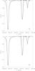 |
Fig. 3 Synthesized line profiles (solid) and the same spectral range observed (dashed) on May 19, 1999 (upper panel) and May 8, 1986 (lower panel). The disk-averaged FTS atlas is overplotted in both panels (dotted lines). Crosses mark the wavelength ranges used for calculating the line equivalent widths. |
3.3. Time-series comparison
Figure 3 shows the whole observed spectral range, obtained during two representative quiet days in the period before and after the change of grating. The disk-averaged FTS atlas (Neckel 1999) is overplotted, so that the change of the line profiles that is due to the grating change is evident. The central depths of all three lines were noticeably smaller before the grating change. The remaining difference between the atlas and observations taken after the grating change is due to the continuum normalization. Crosses mark the spectral ranges used to calculate the EW. They are chosen such that the calculated EW match the EW observed in periods of quiet Sun after 1998. They are kept unchanged for the whole modeled time interval.
Observations taken during the days with the lowest solar activity, in the period before the change of grating (May 1986), were used to find μcut. The comparison of the synthesized and observed EWs gave a value of 0.7 for μcut. For the period after the change of the grating we set μcut = 0.
All synthesized profiles were then convolved with Gaussians so that the instrumental broadening, broadening due to solar rotation, and convective velocity fields were taken into account. These effects are thus approximated by a macroturbulence velocity, in addition to the microturbulence, which was employed unchanged from the values deduced in Sect. 3.2. The broadenings applied to the line profiles were adjusted for each line separately, so that we reproduced the observed line central depths taken at low solar activity. The resulting Gaussian half-widths are given in Table 3. The line broadening was determined separately for the periods before and after the grating change, with values for the latter period being lower. Several factors can play a role here. First, the change of grating and set-up produces a change in the instrumental broadening. Second, by excluding the outer parts of the disk, the influence of the parts of the solar disk that produce more shifted line profiles as a result of solar rotation is changed. Third, before the grating change fewer regions close to the limb were sampled, which experience larger broadening due to convection. As a result of the superposition of these effects, the lines show a 20% larger broadening on average before 1993 (implying a broadening velocity higher by about 10%). Finally, errors introduced in the disk-averaged profiles as a result of the simplicity of our modeling cannot be ruled out, but cannot be estimated either. Assuming LTE also introduces errors.
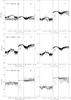 |
Fig. 4 Equivalent widths (left) and central depths (right) of the Fe i 539.32 nm (top), Mn i 539.47 nm (middle), and Fe i 539.52 nm line (bottom) extracted from KPNO observations (crosses) and calculated using our model (solid line). The experimental period (with changing setup parameters) is delimited by vertical lines. The modeled EW values of the Fe i 539.52 nm line are shifted for 0.7 mÅ. |
Figure 4 shows the observed and modeled change of the EW and CD of the three lines over nearly three solar cycles. Vertical lines enclose the period during which the setup of the telescope was frequently changed. The modeled values of the Fe i 539.52 nm line EWs were systematically lower because of the slight blend in its vicinity (see Fig. 3), therefore we corrected for them by adding a constant of 0.7 mÅ.
Combined macroturbulence and instrumental broadening velocity needed to reproduce the line profiles in periods before and after the change of grating, respectively.
It is most conspicuous in Fig. 4 that the shift introduced by the change in the grating is relatively well modeled by the simple technique that we applied. With a single free parameter μcut, we were able to produce the offset in three parameters, the EWs of the three lines.
Another feature in Fig. 4 is the observed variability of the Mn i line is stronger than in the Fe i lines. The variability of the Mn i 539.47 nm line is well reproduced, showing the correct magnitude of the dips of both EW and CD during periods of high activity. The modeled EW and CD of the weak Fe i 539.52 nm line show only a weak change over the solar cycle and match the observations relatively well. The modeled variations are smaller than the scatter of the data. The strong Fe i line, on the other hand, shows a significantly stronger modeled change than is observed. This could be a consequence of the LTE assumption that we made. As a result of the greater formation height of this line (see Table 2), it samples a considerably larger temperature difference between the quiet Sun and the facular model atmosphere (of around 500 K). In LTE this largely compensates for the relative temperature insensitivity of this line. The overestimate of the Fe I 539.32 nm line variability suggests that one of the assumptions made by the model is not met. Given the strength of the line and its high formation height, the departures from LTE might be the main cause.
In total, observations and simulations overlap for 184 and 456 days before and after the change of grating, respectively. Correlation coefficients between observed and computed EW of the Mn line are 0.86 and 0.83, while for the CD they are 0.81 and 0.82 for two periods, respectively. The modeled EW better correlates with observations taken before 1992 than after. One reason is that the observational values obtained after 1993 have intrinsically larger scattering (Livingston et al. 2007).
To some extent as a result of the lack of clear variability in the observations, there is evidently no correlation between the observed and modeled data of the Fe lines, therefore we omit reporting the corresponding correlation coefficients.
4. Conclusions
We calculated the change of the disk-integrated Mn i 539.47 nm line and two neighboring Fe I lines from 1979 to 2009 by using the SATIRE-S model. This model has so far reproduced variations of total and spectral irradiance on timescales of days to multiple solar cycles. However, it has never been tested on individual spectral lines. This test is of particular interest (1) because of the evidence that spectral lines are the dominant contributors to TSI variations over the solar cycle (Mitchell & Livingston 1991; Unruh et al. 1999; Shapiro et al. 2015) and (2) because the recent data from SORCE/SIM (Harder et al. 2009) suggest that the irradiance in the visible varies in antiphase with changes in the TSI.
It was noted previously (Krivova et al. 2006; Unruh et al. 2008) that SATIRE-S might overestimate the variations over the solar cycle of stronger lines that are formed higher up, possibly because NLTE effects are neglected. Indeed, the variation in the profile of the strong Fe I 539.32 nm line modeled here, in particular in the EW, is also overestimated.
At the same time, the observed scatter for the weak Fe I 539.52 nm line is much larger than the modeled change in the line parameters. This is similar to the result found by Penza et al. (2006), who analyzed the second set of photospheric lines observed as part of the “Sun-as-a-Star” program. They employed a simpler model that neglected the heliocentric dependence of the emergent spectra and took certain proxies of solar magnetic activity to estimate the coverage of the solar disk by different features, whereas we employed direct high-resolution full-disk observations. The spectral range analyzed by these authors contained three lines of similar strength as the weak Fe I 539.52 nm line. In general, the scatter in all lines is of the same magnitude, which suggests an instrumental origin (e.g., in determining the exact continuum level, or slightly variable spectral stray light, or slightly variable vignetting with time). The similar trends visible in EW of all these lines in the period from 1978 to 1992 support this conclusion, especially since these trends disappear after the larger grating was installed. However, we cannot exclude that neglecting 3D effects and the impact of the unresolved granular motion on the line profiles introduces an error to our models. This, together with the variability in stronger lines, should be studied with the next generation of irradiance models that will take this into account.
The only line that is insensitive to the velocity field and thus perfect for this type of modeling is Mn I line, whose reconstructed time series of CD and EW agree quite well with the measured parameters. Reproducing the large solar cycle variation of the Mn I line with the SATIRE-S model without optimizing it in any way (the single free parameter of the model remains fixed to the value that was independently determined by Ball et al. 2012) is a success for the model and strengthens the assumption underlying it, namely that variations in TSI and SSI (in the optical wavelength range) are caused by the evolution of the solar surface magnetic field. Furthermore, the fact that SATIRE-S reproduces the correct level of the variation in the Mn line provides strong support to the overall spectral profile of the irradiance variability computed with SATIRE-S. On the one hand, Yeo et al. (2015) have recently demonstrated that the magnitude of the changes in the UV returned by SATIRE-S agrees well with the most stable satellite measurements. On the other hand, since spectral lines determine the amplitude and even the phase of the visible irradiance variations (Shapiro et al. 2015), our finding here indicates that the magnitude of the variability in the visible is also adequate. Finally, the model also reproduces the changes in the TSI that are dominated by changes in the UV and the visible and are measured far more reliably than changes in the spectral irradiance (Yeo et al. 2014a). Thus the model has now been independently tested in the three domains, which leaves little freedom for a significantly different profile of spectral irradiance variability. This further supports the conclusion of Yeo et al. (2014b) that the SATIRE-S model currently presents the most realistic estimate of the solar spectral irradiance variations and is to be preferred for climate studies.
We found a high correlation and a good agreement of the magnitude of solar cycle variations between the observed and reconstructed change in the Mn i line parameters. This implies that the solar cycle variations of the line can be modeled by only taking into account changes in the surface distribution of the solar magnetic features (Danilovic & Vince 2005; Vitas et al. 2009). Since the solar disk coverage by faculae increases from the minimum to the maximum of the solar cycle, the disk-integrated line, in the “Sun-as-a-star” spectrum, becomes weaker during the solar cycle maximum. This explains why this manganese line mimics the behavior of Ca ii K and Mg ii k lines, which are well-known plage and faculae indicators. The influence of sunspots is negligible. No additional temperature change in the quiet-Sun component is necessary.
Acknowledgments
We thank Rob Rutten for revising the manuscript very carefully and giving helpful instructions. This work was partly supported by the German Federal Ministry of Education and Research under project 01LG1209A and by the BK21 plus program through the National Research Foundation (NRF) funded by the Ministry of Education of Korea.
References
- Asplund, M., Nordlund, Å., Trampedach, R., Allen de Prieto, C., & Stein, R. F. 2000, A&A, 359, 729 [NASA ADS] [Google Scholar]
- Ball, W. T., Unruh, Y. C., Krivova, N. A., et al. 2012, A&A, 541, A27 [NASA ADS] [CrossRef] [EDP Sciences] [Google Scholar]
- Balthasar, H. 1988, A&AS, 72, 473 [NASA ADS] [Google Scholar]
- Bergemann, M., & Gehren, T. 2007, A&A, 473, 291 [NASA ADS] [CrossRef] [EDP Sciences] [Google Scholar]
- Brault, J. W., Slaughter, C. D., Pierce, A. K., & Aikens, R. S. 1971, Sol. Phys., 18, 366 [NASA ADS] [CrossRef] [Google Scholar]
- Brodzinski, T., Kronfeldt, H.-D., Kropp, J.-R., & Winkler, R. 1987, Physik D, 7, 161 [Google Scholar]
- Condon, E. U., & Shortley, G. H. 1963, The Theory of Atomic Spectra (Cambridge: University Press), 242 [Google Scholar]
- Danilovic, S., & Vince, I. 2005, Mem. Soc. Astron. It., 76, 949 [NASA ADS] [Google Scholar]
- Danilovic, S., Vince, I., Vitas, N., & Jovanovic, P. 2005, Serb. Astron. J., 170, 79 [Google Scholar]
- Davis, S. J., Wright, J. J., & Balling, L. C. 1971, Phys. Rev. A, 3, 1220 [NASA ADS] [CrossRef] [Google Scholar]
- Domingo, V., Ermolli, I., Fox, P., et al. 2009, Space Sci. Rev., 145, 337 [Google Scholar]
- Doyle, J. G., Jevremovic, D., Short, C. I., et al. 2001, A&A, 369, L13 [NASA ADS] [CrossRef] [EDP Sciences] [Google Scholar]
- Elste, G. 1986, Sol. Phys., 107, 47 [Google Scholar]
- Elste, G., & Teske, R. G. 1978, Sol. Phys., 59, 275 [NASA ADS] [CrossRef] [Google Scholar]
- Ermolli, I., Matthes, K., Dudok de Wit, T., et al. 2013, Atm. Chem. Phys., 13, 3945 [NASA ADS] [CrossRef] [Google Scholar]
- Fligge, M., Solanki, S. K., & Unruh, Y. C. 2000, A&A, 353, 380 [NASA ADS] [Google Scholar]
- Fontenla, J., White, O. R., Fox, P. A., Avrett, E. H., & Kurucz, R. L. 1999, ApJ, 518, 480 [NASA ADS] [CrossRef] [Google Scholar]
- Fröhlich, C., Romero, J., Roth, H., et al. 1995, Sol. Phys., 162, 101 [NASA ADS] [CrossRef] [Google Scholar]
- Frutiger, C. C., Solanki, S. K., Fligge, M., & Bruls, J. H. M. J. 2000, A&A, 358, 1109 [NASA ADS] [Google Scholar]
- Grossmann-Doerth, U., Larsson, B., & Solanki, S. K. 1988, A&A, 204, 266 [NASA ADS] [Google Scholar]
- Gurtovenko, E. A., & Kostyk, R. I. 1989, Fraunhofer Spectrum and System of Solar Oscillator Strengths, Naukova dumka (Kiev), 200 [Google Scholar]
- Harder, J. W., Fontenla, J. M., Pilewskie, P., Richard, E. C., & Woods, T. N. 2009, Geophys. Res. Lett., 36, 7801 [NASA ADS] [CrossRef] [Google Scholar]
- Holweger, H., Gehlsen, M., & Ruland, F. 1978, A&A, 70, 537 [NASA ADS] [Google Scholar]
- Krivova, N. A., Solanki, S. K., Fligge, M., & Unruh, Y. C. 2003, A&A, 399, L1 [NASA ADS] [CrossRef] [EDP Sciences] [Google Scholar]
- Krivova, N. A., Solanki, S. K., & Floyd, L. 2006, A&A, 452, 631 [NASA ADS] [CrossRef] [EDP Sciences] [Google Scholar]
- Krivova, N. A., Solanki, S. K., Wenzler, T., & Podlipnik, B. 2009, J. Geophys. Res., 114, [Google Scholar]
- Krivova, N. A., Solanki, S. K., & Schmutz, W. 2011, A&A, 529, A81 [NASA ADS] [CrossRef] [EDP Sciences] [Google Scholar]
- Kupka, F., Piskunov, N., Ryabchikova, T. A., Stempels, H. C., & Weiss, W. W. 1999, A&AS, 138, 119 [NASA ADS] [CrossRef] [EDP Sciences] [MathSciNet] [PubMed] [Google Scholar]
- Kurucz, R. L. 1991, Stellar Atmospheres – Beyond Classical Models, Proc. Advanced Research Workshop, Trieste, Italy (Dordrecht, D. Reidel Publishing Co.), 441 [Google Scholar]
- Kurucz, R. L. 1992, The Stellar Populations of Galaxies, International Astronomical Union, eds. B. Barbuy, & A. Renzini (Dordrecht: Kluwer Academic Publishers), 225, 149 [Google Scholar]
- Livingston W. 1992, in Proc. Workshop on the Solar Electromagnetic Radiation Study for Solar Cycle 22, ed. R. F. Donnelly, 11 [Google Scholar]
- Livingston, W., & Wallace, L. 1987, ApJ, 314, 808 [NASA ADS] [CrossRef] [Google Scholar]
- Livingston, W., Wallace, L., White, O. R., & Giampapa, M. S. 2007, ApJ, 657, 1137 [NASA ADS] [CrossRef] [Google Scholar]
- Livingston, W., White, O. R., Wallace, L., & Harvey, J. 2010, Mem. Soc. Astron. It., 81, 643 [NASA ADS] [Google Scholar]
- Magain, P. 1986, A&A, 163, 135 [NASA ADS] [Google Scholar]
- Malanushenko, O., Jones, H. P., & Livingston, W. 2004, Multi-Wavelength Investigations of Solar Activity, 223, 645 [NASA ADS] [Google Scholar]
- Mitchell, W. E., Jr., & Livingston, W. C. 1991, ApJ, 372, 336 [NASA ADS] [CrossRef] [Google Scholar]
- Neckel, H., 1999, Sol. Phys., 184, 421 [NASA ADS] [CrossRef] [Google Scholar]
- Penza, V., Pietropaolo, E., & Livingston, W. 2006, A&A, 454, 349 [NASA ADS] [CrossRef] [EDP Sciences] [Google Scholar]
- Rodriguez Hidalgo, I., Collados, M., & Vazquez, M. 1994, A&A, 283, 263 [NASA ADS] [Google Scholar]
- Shapiro, A. I., Solanki, S. K., Krivova, N. A., et al. 2015, A&A, 581, A116 [NASA ADS] [CrossRef] [EDP Sciences] [Google Scholar]
- Shchukina, N., & Trujillo Bueno, J. 2001, ApJ, 550, 970 [NASA ADS] [CrossRef] [Google Scholar]
- Solanki, S. K., Krivova, N. A., & Wenzler, T. 2005, Adv. Space Res., 35, 376 [Google Scholar]
- Solanki, S. K., Krivova, N. A., & Haigh, J. D. 2013, ARA&A, 51, 311 [NASA ADS] [CrossRef] [Google Scholar]
- Unruh, Y. C., Solanki, S. K., & Fligge, M. 1999, A&A, 345, 635 [NASA ADS] [Google Scholar]
- Unruh, Y. C., Krivova, N. A., Solanki, S. K., Harder, J. W., & Kopp, G. 2008, A&A, 486, 311 [NASA ADS] [CrossRef] [EDP Sciences] [Google Scholar]
- Vince, I., Vince, O., Ludmány, A., & Andriyenko, O. 2005a, Sol. Phys., 229, 273 [NASA ADS] [CrossRef] [Google Scholar]
- Vince, I., Gopasyuk, O., Gopasyuk, S., & Vince, O. 2005b, Serbian Astron. J., 170, 115 [NASA ADS] [CrossRef] [Google Scholar]
- Vitas, N. 2005, Mem. Soc. Astron. It. Supp., 7, 164 [Google Scholar]
- Vitas, N., & Vince, I. 2007, The Physics of Chromospheric Plasmas, 368, 543 [NASA ADS] [Google Scholar]
- Vitas, N., Viticchiè, B., Rutten, R. J., & Vögler, A. 2009, A&A, 499, 301 [NASA ADS] [CrossRef] [EDP Sciences] [Google Scholar]
- Wallace, L., Hinkle, K., & Livingston, W. 2007, An Atlas of the Spectrum of the Solar Photosphere from 13 500 to 33 980 cm-1 (2942 to 7405 Å), Published by NSO [Google Scholar]
- Wenzler, T., Solanki, S. K., Krivova, N. A., & Fluri, D. M. 2004, A&A, 427, 1031 [NASA ADS] [CrossRef] [EDP Sciences] [Google Scholar]
- Wenzler, T., Solanki, S. K., & Krivova, N. A. 2005, A&A, 432, 1057 [NASA ADS] [CrossRef] [EDP Sciences] [Google Scholar]
- Wenzler, T., Solanki, S. K., Krivova, N. A., & Fröhlich, C. 2006, A&A, 460, 583 [NASA ADS] [CrossRef] [EDP Sciences] [Google Scholar]
- Yeo, K. L., Krivova, N. A., Solanki, S. K., & Glassmeier, K. H. 2014a, A&A, 570, A85 [NASA ADS] [CrossRef] [EDP Sciences] [Google Scholar]
- Yeo, K. L., Krivova, N. A., & Solanki, S. K. 2014b, Space Sci. Rev., 186, 137 [NASA ADS] [CrossRef] [Google Scholar]
- Yeo, K. L., Ball, W. T., Krivova, N. A., et al. 2015, J. Geophys. Res., 120 DOI: 10.1002/2015JA021277 [Google Scholar]
All Tables
Line characteristics: wavelength, transition, oscillator strength, and excitation energy.
Combined macroturbulence and instrumental broadening velocity needed to reproduce the line profiles in periods before and after the change of grating, respectively.
All Figures
|
Fig. 1 Illustration of flux calculations for the period before 1993 when the old grating was used. The two horizontal lines delimit the part of the disk that illuminates the grating. The dashed circle corresponds to μ = μcut. |
| In the text | |
|
Fig. 2 Left-hand side: profiles of Fe i 539.32 nm, Mn i 539.47 nm, and Fe i 539.52 nm lines at the disk center, from top to bottom. The profiles are computed in the following model atmospheres: quiet Sun (dashed), faculae (dotted), penumbrae (double-dot-dashed), and umbrae (dash-dotted). FTS atlas profiles are overplotted (solid curves). Right-hand side: center-to-limb variation of the EW of the lines. Symbols distinguish between the EW resulting from different model atmospheres: quiet Sun (plus signs), faculae (asterisks), penumbrae (crosses), and umbrae (squares). Diamonds with error bars are values observed in the quiet Sun. |
| In the text | |
|
Fig. 3 Synthesized line profiles (solid) and the same spectral range observed (dashed) on May 19, 1999 (upper panel) and May 8, 1986 (lower panel). The disk-averaged FTS atlas is overplotted in both panels (dotted lines). Crosses mark the wavelength ranges used for calculating the line equivalent widths. |
| In the text | |
|
Fig. 4 Equivalent widths (left) and central depths (right) of the Fe i 539.32 nm (top), Mn i 539.47 nm (middle), and Fe i 539.52 nm line (bottom) extracted from KPNO observations (crosses) and calculated using our model (solid line). The experimental period (with changing setup parameters) is delimited by vertical lines. The modeled EW values of the Fe i 539.52 nm line are shifted for 0.7 mÅ. |
| In the text | |
Current usage metrics show cumulative count of Article Views (full-text article views including HTML views, PDF and ePub downloads, according to the available data) and Abstracts Views on Vision4Press platform.
Data correspond to usage on the plateform after 2015. The current usage metrics is available 48-96 hours after online publication and is updated daily on week days.
Initial download of the metrics may take a while.