| Issue |
A&A
Volume 586, February 2016
|
|
|---|---|---|
| Article Number | A99 | |
| Number of page(s) | 8 | |
| Section | Interstellar and circumstellar matter | |
| DOI | https://doi.org/10.1051/0004-6361/201527754 | |
| Published online | 01 February 2016 | |
Steepening of the 820 μm continuum surface brightness profile signals dust evolution in TW Hydrae’s disk
1 Leiden Observatory, Leiden University, PO Box 9513, 2300 RA Leiden, The Netherlands
e-mail: michiel@strw.leidenuniv.nl
2 Harvard-Smithsonian Center for Astrophysics, 60 Garden Street MS42, Cambridge, MA 02138, USA
Received: 16 November 2015
Accepted: 16 December 2015
Context. Grain growth in planet-forming disks is the first step toward the formation of planets. The growth of grains and their inward drift leaves a distinct imprint on the dust surface density distribution and the resulting surface brightness profile of the thermal continuum emission.
Aims. We determine the surface brightness profile of the continuum emission using resolved observations at millimeter wavelengths of the disk around TW Hya, and infer the signature of dust evolution on the surface density and dust opacity.
Methods. Archival ALMA observations at 820 μm on baselines up to 410 kλ are compared to parameterized disk models to determine the surface brightness profile.
Results. Under the assumption of a constant dust opacity, a broken radial power law best describes the dust surface density with a slope of −0.53 ± 0.01 from the 4.1 au radius of the already known inner hole to a turn-over radius of 47.1 ± 0.2 au, steepening to −8.0 ± 0.1 at larger radii. The emission drops below the detection limit beyond ~60 au.
Conclusions. The shape of the dust surface density is consistent with theoretical expectations for grain growth, fragmentation, and drift, but its total dust content and its turn-over radius are too large for TW Hya’s age of 8–10 Myr even when taking into account a radially varying dust opacity. Higher resolution imaging with ALMA of TW Hya and other disks is required to establish whether unseen gaps associated with, e.g., embedded planets trap grains at large radii or whether locally enhanced grain growth associated with the CO snow line explains the extent of the millimeter continuum surface brightness profile. In the latter case, population studies should reveal a correlation between the location of the CO snow line and the extent of the millimeter continuum. In the former case, and if CO freeze-out promotes planet formation, this correlation should extend to the location of gaps as well.
Key words: accretion, accretion disks / protoplanetary disks / circumstellar matter / submillimeter: planetary systems / dust, extinction
© ESO, 2016
1. Introduction
Within the core accretion scenario, the formation of planets starts inside disks around newly formed stars with the coagulation of (sub)micron-sized dust grains into larger objects (see, e.g., Lissauer & Stevenson 2007, for a review). Evidence for grain growth follows from the spectral slope from submillimeter to centimeter wavelengths (e.g., Draine 2006) and has been found toward many disks (Beckwith et al. 1990; Andrews & Williams 2005; Rodmann et al. 2006; Lommen et al. 2009; Ricci et al. 2010a,b, 2011; Mann & Williams 2010; Guilloteau et al. 2011; Ubach et al. 2012). As grains grow to millimeter sizes, they start to decouple dynamically from the gas and, no longer supported by gas pressure, begin to feel the headwind of the gas and drift inward (Whipple 1972; Weidenschilling 1977). This results in radially more compact millimeter continuum emission (roughly probing millimeter-sized dust) than near-infrared scattered light (probing sub-micron-sized dust) and CO (probing the cold gas), as detected in an increasing number of disks (Panić et al. 2009; Andrews et al. 2012; de Gregorio-Monsalvo et al. 2013; Walsh et al. 2014). The high sensitivity of the Atacama Large Millimeter/submillimeter Array (ALMA) allows detailed investigation of the radial distribution of millimeter-sized grains and critical comparison to theoretical expectations of their growth and dynamics.
One of the first disks for which radial migration of millimeter-sized dust was inferred is found around the nearby T Tauri star TW Hya (Andrews et al. 2012). At a distance of 53.7 ± 6.2 pc (Hipparcos; van Leeuwen 2007), TW Hya is the closest gas- and dust-rich planet-forming disk; it is observed close to face-on with an inclination of 7° ± 1° (Qi et al. 2004; Hughes et al. 2011; Rosenfeld et al. 2012). TW Hya has a mass of 0.55 ± 0.15 M⊙ and, although some uncertainty exists (Vacca & Sandell 2011), an estimated age of 8–10 Myr (Hoff et al. 1998; Webb et al. 1999; de la Reza et al. 2006; Debes et al. 2013). Its disk has a gas mass of at least 0.05 M⊙ as inferred from the emission of HD (Bergin et al. 2013), consistent with a gas-to-dust ratio of 100 and the derived dust mass of 2–6 ×10⁻⁴M⊙ (Calvet et al. 2002; Thi et al. 2010). The outer radius of the disk as seen at near-infrared wavelengths and in the emission of CO is ~200–280 au (Weinberger et al. 2002; Qi et al. 2004; Andrews et al. 2012; Debes et al. 2013). From the spectral energy distribution (SED) an inner hole in the disk of ~4 au was found (Calvet et al. 2002; Hughes et al. 2007; Menu et al. 2014). Andrews et al. (2012) show that millimeter-sized grains, as traced by 870 μm SMA observations, extend out only to ~60 au, indicating significant radial inward drift. Menu et al. (2014) found a population of even larger grains at smaller radii from 7 mm JVLA observations. At near-infrared wavelengths, Debes et al. (2013) show a depression of emission around 80 au, while Akiyama et al. (2015) detected structure in polarized scattered light at radii of 10–20 au possibly indicating a gap, or changes in the scale height or opacity of micron-sized grains.
In this paper we reanalyze archival ALMA Cycle 0 data of the 820 μm (365.5 GHz) continuum emission of TW Hya with an angular resolution of ~0 4. This observing wavelength is near 870 μm, the wavelength used by Andrews et al. (2012) to infer the 60 au outer radius for millimeter-sized grains. We do not consider available ALMA continuum data at 106 GHz and 663 GHz because we aim to make a direct comparison to the 870 μm SMA data without the added degeneracy between dust surface density and dust emissivity as a function of wavelength. The sensitivity of the archival ALMA data allows detailed comparison of the continuum visibilities as a function of deprojected baseline length with parameterized models of the disk. Section 2 presents the data and describes how the visibilities vary with deprojected baseline length. Section 3 describes our disk model and the fitting methods, yielding the radial surface brightness profile of millimeter-sized grains as well as the underlying dust surface density and opacity. Section 4 discusses our results in the light of theoretical models of dust grain growth, fragmentation, and transport, and Sect. 5 summarizes our findings.
2. Observations and data reduction
The ALMA archive contains two Cycle 0 data sets with continuum observations of TW Hya near 870 μm. These data sets are 2011.0.00340.S (hereafter 340.S), covering wavelengths of 804–837 μm (frequencies of 348–373 GHz), a total bandwidth of 0.94 GHz, baselines up to 370 m (460 kλ), and a total on-source integration time of 5449 s; and 2011.0.00399.S (hereafter 399.S), covering 867–898 μm (334–346 GHz), a total bandwidth of 0.24 GHz, baselines up to 345 m (430 kλ), and a total on-source integration time of 4615 s. For both data sets, 3C 279 and J0522−364 served as bandpass calibrators; Ceres, and for a part of data set 399.S, Titan, as flux calibrators; and J1037−295 as gain calibrator. Median system temperatures were 230–260 K for S.340 and 110–130 K for S.399. The 340.S data were previously presented by Qi et al. (2013), who do not analyze the continuum emission in detail.
After verifying the calibration of these data sets, to improve the complex gain calibration we iteratively performed self-calibration on the continuum down to solution intervals of 60 s. We use CASA 4.2.1 for the calibration. We reach noise levels of 0.50 mJy beam-1 (340.S) and 0.59 mJy beam-1 (399.S). Uniformly weighted synthesized beams are  (340.S) and
  (399.S). Integrated fluxes of 1.7 Jy (340.S) and 1.3 Jy (399.S) are found.
In the remainder of this paper, we focus on data set 340.S which has slightly higher resolution and lower noise. Although we can combine both data sets into a single set at an effective observing wavelength, with a ~30% lower resulting noise, we instead prefer to use data set 399.S to independently confirm our results and other than that, we do not discuss this data set further in this paper. Figure 1 shows the continuum image obtained from data set 340.S.
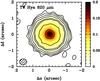 |
Fig. 1 820 μm (365.5 GHz) continuum of TW Hya based on data set 2011.0.00340.S. We reimaged these data, and obtain a result indistinguishable from (Qi et al. 2013). The image construction employed self-calibration and uniform weighting. The resulting beam size, indicated in the lower left, is |
Adopting a position angle for the disk’s major axis of 155° (east of north) and an inclination of + 6° (Qi et al. 2013; Rosenfeld et al. 2012), we derive average continuum visibilities (real and imaginary part) in 41 10-kλ wide radial bins of deprojected baseline length. We use the equations of Berger & Segransan (2007, as referenced in Walsh et al. 2014) to carry out the deprojection. Given the near face-on orientation of TW Hya’s disk, the deprojection corrections are small.
Figure 2 plots the real and imaginary parts of the continuum visibilities against the deprojected baseline length. The imaginary parts are all zero to within the accuracy, indicating that the emission is symmetric around the source center at the resolution of our observations. Apart from the much higher signal-to-noise ratio, the real part of the visibilities show a behavior similar to that shown by Andrews et al. (2012), with a drop off from 1.72 Jy at the shortest baselines to a minimum of 0.057 Jy near 190 kλ, followed by a second maximum of 0.123 Jy around 275 kλ and a subsequent decrease to 0.028 Jy at our longest baseline of 410 kλ. The data of Andrews et al. (2012) continue to longer baselines of 600 kλ with fluxes approaching 0 Jy.
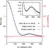 |
Fig. 2 Real (black points) and imaginary (red points) parts of the visibilities of project 340.S (previously presented in Qi et al. 2013) in Jy vs deprojected baseline length in kλ. The inset shows the region of 120–420 kλ in greater detail. The dashed black curve shows the recalculated single power-law model of Andrews et al. (2012, their model pC), which fails to reproduce the data on baselines >290 kλ. A much better fit is found for a broken power-law model described in Sect. 3 (solid blue curve). Because both models are symmetric, the imaginary parts of their visibilities are all 0 (not shown). |
We overplot the data with the model presented by Andrews et al. (2012, their model pC) which they find to best fit the continuum data. We recalculate the model at the exact observing wavelengths of the ALMA data. Our model is geometrically thin and uses only the midplane temperatures as calculated by Andrews et al. (2012) (see Sect. 3). Our model curve therefore differs in detail from the one shown by Andrews et al. (2012), but qualitatively shows the same behavior. In particular, it fits the data well out to baselines of 290 kλ but severely underpredicts the emission on baselines of 300 and 400 kλ, corresponding to angular scales of  –
– (27–37 au). In the next section we attempt to find a model description that provides a better fit.
3. Model fitting
To further investigate the disk structure that best describes the observed emission, we consider the deprojected and radially binned real visibilities of data set 340.S. We fit to the 41 data points plotted in Fig. 2 rather than the full set of complex visibilities to speed up calculations. Since the observed emission is symmetric (imaginary visibilities are all 0) and the 41 data points in Fig. 2 fully sample the curve and do not average out any detected asymmetric structure, this simplification is allowed. As a consequence of using only the binned visibilities, our fitting places relatively little weight on the shortest baselines, which represent the total flux. Because we are primarily interested in the spatial distribution of the emission, rather than the total amount, our results are not affected. However, even a small discrepancy in total flux would be accentuated if we would calculate a residual image. For this reason, we refrain from imaging the residuals and exclusively work with the visibilities.
The real part of the visibilities, V, are related to the intensity distribution of the source by  (1)where ruv is the baseline length, Iν(R) is the intensity as a function of radius R, and J0 the zeroth order Bessel function of the first kind (see, e.g., Hughes et al. 2007). We solve the integral in Eq. (1) by summation using a step size of 0.1 au, which was found to be sufficiently small.
The intensity Iν(R) follows from the expression  (2)where Bν(T(R)) is the Planck function, T(R) is the dust temperature, and τ(R) is the dust optical depth which is given by the product of the dust surface density Σ, the dust opacity κ at the observing wavelength, and cos i, where i is the inclination. The factor cos i is very close to unity for TW Hya.
We follow the midplane temperature as calculated by Andrews et al. (2012), which reproduces the observed SED. Here, T(R) is characterized by a very steep drop off in the inner few au, with T(R) ∝ R− q0 with q0 = 2.6, followed by a very shallow decrease across the remainder of the disk, with T(R) ∝ R− q1 and q1 = 0.26. Physically, this corresponds to the stellar radiation being stopped by the high opacity in the inner few au of the disk just outside the inner hole, and the remainder of the disk being heated indirectly by stellar radiation absorbed in the disk surface and reradiated vertically (e.g., Chiang & Goldreich 1997). In our model, the temperature at the turnover radius, R0 (7 au), T0, is a free parameter. In all cases, we find best-fit values for T0 close to the values found by Andrews et al. (2012). Furthermore, R0 is much smaller than the resolution of our data, and T0 is degenerate with the optical depth τ(R). Therefore their exact values do not change our results. The steep rise of the temperature in the inner few au adds an unresolved component to the continuum emission. This provides a vertical offset to the real part of the visibilities. Indeed, the observed real part of the visibilities never become negative (Fig. 2), showing that the sharp increase in temperature at small radii is essential in our model even if we do not resolve these scales.
We choose to describe the optical depth τ(R) as the product of a constant dust opacity κ365.5 and a radially varying dust surface density distribution Σ(R). For the dust opacity at the average observing wavelength of 365.5 GHz κ365.5, we adopt the same value as employed by Andrews et al. (2012), κ365.5 = 3.4 cm2 g-1 (dust). We describe the dust surface density Σ(R) as a (set of) radial power law(s) between an inner radius Rin and an outer radius Rout. In Sect. 4.1 we further discuss what happens if also κ varies radially, as would be naturally expected.
Model parameters.
Table 1 lists the fixed and 4 or 6 (depending on the model) free parameters of our model. Estimates of the parameters follow from a Markov chain Monte Carlo (MCMC) exploration of the parameter space, minimizing  , where xi and yi are the 41 observed and modeled binned real visibilities, and σi the observed dispersion in each of the bins. These σi correspond to the error on the averaged real visibilities and follow from the dispersion of the data points in the bin divided by the square root of the number of data points. Any undetected asymmetric structures also contribute to σi, which ranges from 2.0 to 12.0 mJy, with a median value of 3.0 mJy. We use the emcee1 implementation of the MCMC method, which uses affine invariant ensemble sampling (Goodman & Weare 2010; Foreman-Mackey et al. 2013). Figure A.1 plots the results.
Assuming a single radial power law for the surface density, the relevant free parameters in our model are the surface density distribution Σ(R), the inner hole radius Rin, and the outer radius Rout. In all cases we find inner radii on the order of a few au, consistent with SED estimates of the inner hole. The best-fit model of Andrews et al. (2012, their model pC) has Σ(R) ∝ R-0.75 and a surface density of Σ0 of 0.39 g cm-2 at 10 au. Keeping this Σ0 fixed and using a single power power law for the radial dependence (Σ ∝ R− p0), we find very similar values as Andrews et al. (2012) for the slope (p0 = 0.70 ± 0.01 vs. 0.75) and outer radius (Rout = 55.7 ± 0.1 au vs. 60 au; see Table 1). The quoted errors on the parameters are formal fitting errors, only meaningful within the model assumptions. The emission in Fig. 1 is convolved with the synthesized beam and therefore appears to extend beyond the value for Rout found from the visibilities (57 au, corresponding to  ). Figure 2 shows the model curve corresponding to the single power law fit. This curve is similar, but not identical, to the curve for model pC in Andrews et al. (2012). Although the parameters are nearly identical, our model is vertically isothermal, unlike model pC, resulting in a slightly different curve. Regardless, both models have equal problems in reproducing the visibilities on baselines of 300–400 kλ.
After this single radial power law as a description for the surface density, the next simplest model consists of a broken power law, with Σ(R) ∝ R− p0 inside a radius Rbreak and Σ(R) ∝ R− p1 outside this radius. This adds two free parameters to the model p1 and Rbreak. A very good fit to the data is found (Fig. 2, Table 1 and Fig. A.2). In this best-fit model, the radial drop off of the surface density is initially modest (p0 = 0.53 ± 0.01) out to a radius of 47.1 ± 0.2 au, followed by a very sharp drop at larger radii (p1 = 8.0 ± 0.1). Given the fast drop of the surface density, no useful constraint on the outer radius is found (200 ± 55 au), as the emission drops below the detection limit. This fit is significantly better than the single power law fit, with respective χ2 values of 1437 and 283. A likelihood ratio test indicates that the broken power law model describes the data better than the single power law model with a probability lager than 0.999.
The broken power law solution found above should not be confused with the exponentially tapered models that are often used (see, for example, Hughes et al. 2008). Such models are described by a surface density Σ = Σc(R/Rc)− γexp [−(R/Rc)2−γ]. Andrews et al. (2012) already show that exponentially tapered models do not fit the millimeter continuum visibilities of TW Hya: there are no values of γ that give a sufficiently shallow drop off of Σ at small R and a sufficiently steep fall off at large R. Only our broken power law can combine these slopes.
In this analysis, we have parameterized the emission with a constant dust opacity κ and a radially varying surface density Σ(R). We stress that our real constraints are on the dust optical depth τ(R) = κΣ. This optical depth follows the same radial broken power law found above. The functional description of the surface brightness profile is more complex, since following Eq. (2) it also includes the slope of the temperature via the Planck function and the slope of the optical depth via the factor (1−exp(−τ)). The optical depth drops from 2.1 at 4.1 au to 0.57 at 47 au, making the emission moderately optically thick and preventing us from taking the limit for small τ, limτ → 0(1−exp(−τ)) = τ.
4. Discussion
4.1. Dust drift
The broken power law distribution obtained for the dust surface density resembles predictions from Birnstiel & Andrews (2014) who consider the effects of radial drift and gas drag on the growing grains. At late time (~0.5–1 Myr in their models), the dust surface density follows a slope of approximately −1 out to ~50 au, after which it steepens to approximately −10. Our inferred surface density profile, although different in detail, shows a similar steeping, further strengthening the suggestion of Andrews et al. (2012) that the grains in TW Hya’s disk have undergone significant growth and drift. However, Birnstiel & Andrews (2014) consider the total dust surface density while our fit is essentially to the 820 μm continuum optical depth profile. This is dominated by grains of roughly 0.1–10 mm (Draine 2006) but grains of all sizes contribute. As noted by Birnstiel & Andrews (2014), the total dust surface density consist of a radially varying population of dust at different sizes, with larger grains having more compact distributions than smaller grains. This is certainly the case for TW Hya, given that grains small enough to scatter near-infrared light extend out to 200–280 au (Debes et al. 2013) while 7 mm observations by Menu et al. (2014) show emission concentrated toward only the inner several au. From observations at a single wavelength we cannot infer both the dust surface density and the dust opacity as a function of radius.
Various authors describe simulations of grain evolution including growth, fragmentation, and drift (e.g., see Testi et al. 2014, for a review). Pinilla et al. (2015) follow the description of Birnstiel et al. (2010) to describe the advection-diffusion differential equation for the dust surface density simultaneously with the growth, fragmentation, and erosion of dust grains via grain-grain collisions. We do not perform a detailed simulation of the TW Hya disk here, since this would require knowledge of the gas surface density distribution and comparison to multiwavelength continuum observations. Instead, we note that any simulation of realistic disks using the prescriptions of Pinilla et al. (2015) results in a very low 820 μm continuum surface brightness and in radial profiles that have turnover radii Rbreak ≲ 20 au at ages >5 Myr and therefore cannot explain the observations for the 8–10 Myr of TW Hya. This age vs. surface brightness (extent) problem was already noted before (e.g., Pinilla et al. 2012, 2015; Testi et al. 2014). The conundrum of TW Hya’s surface brightness profile is that it resembles in shape the signatures of grain evolution and drift while in in flux and size it is too bright and extended for these same mechanisms to have operated over the 8–10 Myr lifetime of the disk.
One possible explanation is that TW Hya’s disk was originally much more massive and larger than the 200–280 au now seen. However, to have a turn-over radius of ~50 au, after 10 Myr, requires an initial disk size of 800–1000 au and a mechanism to remove all CO and small dust outside 200 au over the past 10 Myr to match current observations of CO line emission and near-infrared scattered light. We do not consider this a likely scenario.
4.2. The presence of unseen gaps
Another possibility to explain the apparent youth of TW Hya’s disk both in terms of the turn-over radius of the surface brightness distribution of the millimeter continuum and its significant gas and dust content lies in comparison to the recent high resolution imaging results of millimeter continuum emission of HL Tau (ALMA Partnership et al. 2015). HL Tau is a very young disk (<1 Myr), but its millimeter continuum image shows a remarkable set of bright and dark rings. The presence of these rings have been variously interpreted as the result of gap clearing by embedded planets (Dipierro et al. 2015; Dong 2015; Pinte et al. 2016), secular gravitational instabilities (Youdin 2011; Takahashi & Inutsuka 2014), or emissivity depressions due to accelerated grain growth to decimeter sizes at the location of the frost lines of dominant ices and clathrates (Zhang et al. 2015; Okuzumi et al. 2015).
Millimeter-sized grains are known to become trapped outside gaps in so-called transitional disks because of the reversed pressure gradient (e.g., van der Marel et al. 2013; Casassus et al. 2013). Therefore, one or more embedded planets inside the TW Hya disk could have trapped millimeter-sized grains and prevented further inward migration. This mechanism has been invoked by Pinilla et al. (2012), who show that even small pressure maxima are sufficient to slow down the inward migration of millimeter-sized dust.
We investigated if the currently available ALMA data place constraints on the presence of gaps inside the TW Hya disk, other than the known gap inside ~4 au. Starting with the two-slope model, we include a gap centered on 20 au characterized by a Gaussian width and a depth. We choose the value of 20 au to be near the center of the extent of the millimeter-sized grains. We then repeat the procedure of the previous section to find the best-fit parameters for a series of gap widths and depths. By optimizing the other free model parameters we allow these to maximally compensate for the effect of the presence of the gap on the visibilities. We find that we can exclude, as defined by an increase of the χ2 value by a factor of two or more, models with gaps that are entirely empty with FWHM widths of more than 6.6 au and models with gaps that have only a depth of 80% to widths of 16.6 au. Assuming a gap width of 5 Hill radii, such gaps correspond to planet masses of 0.7–10 MJup (Dodson-Robinson & Salyk 2011). For comparison, the widths and depths of the gaps in HL Tau are well within the allowed range. We conclude that TW Hya’s disk may very well contain planet-induced gaps as detected toward HL Tau, which are capable of halting further inward migration of grains and explain the observed millimeter continuum surface brightness profile.
4.3. Dust temperature and the CO snow line
The discussion above attributes the characteristics of the distribution of the millimeter-wave continuum to the surface density distribution and opacity of the grains. According to Eq. (2) the explanation could equally well lie with the dust temperature. At radii inside the turn-over of the emission, up to 47 au, the disk is known to be cold, <20 K, as witnessed by the CO freeze-out probed by N2H+ emission (Qi et al. 2013). A shallow surface density distribution combined with a steep temperature drop off outside 47 au cannot explain the observations, since this requires unrealistically low temperatures (≪10 K). A steeper density distribution combined with a temperature rise around 30–40 au followed by a return to nominal temperatures can fit the observations, but requires temperatures as high as 70 K, clearly inconsistent with the detection of N2H+ that would be rapidly destroyed by gas-phase CO at such temperatures.
The N2H+ data from Qi et al. (2013) place the CO snow line at 30 au. Just outside this snow line, grain growth may receive a boost by the accumulation of frost resulting from mixing of material across the snow line. This cold-finger effect was earlier described by Meijerink et al. (2009) and invoked by Zhang et al. (2015) to explain the dark rings in the HL Tau millimeter continuum image as locations of growth to decimeter-sized particles at the location of frost lines. Similarly in TW Hya, the location of the turn-over radius in the millimeter emission may be determined, not by the inward migration of millimeter-sized grains, but by a local enhancement of growth of (sub) micron-sized grains to millimeter sized grains in the 30–47 au region outside the CO snow line. If the efficiency of grain growth is locally sufficiently enhanced, this may increase the dust opacity at 820 μm and explain the observed surface brightness profile. Zhang et al. (in prep.) present an analysis of four protoplanetary disks with high resolution continuum observations, and find that regions just beyond CO snow lines show locally enhanced continuum emission. Detailed modeling of grain growth and drift in the presence of ices and the resulting dust opacity is required to further explore this mechanism. If this mechanism is indeed effective, population studies of disks should reveal a correlation between the location of the CO snow lines2 and the sizes of the millimeter continuum emission disk.
5. Summary
We analyzed archival ALMA Cycle 0 365.5 GHz continuum data with baselines up to 410 kλ and conclude the following.
-
1.
The interferometric visibilities are described by a disk with a broken power law radial surface density distribution and constant dust opacity, with slopes of −0.53 ± 0.01 and −8.0 ± 0.2 and a turn-over radius of 47.1 ± 0.2 au. The outer radius is unconstrained as the emission drops below the detection limit beyond ~57 au.
-
2.
Under the assumption of a constant dust opacity κ, the shape of the corresponding surface density distribution resembles the one expected in the presence of grain growth and radial migration for late times as calculated by Birnstiel & Andrews (2014).
-
3.
The total surface brightness and the turn-over radius of 47 au are too large for a source age of 8–10 Myr. This implies that either the disk formed with a much larger size and mass, that one or more unseen embedded planets have opened gaps and halted inward drift of millimeter-sized grains, or that the region outside the CO snow line at radii of 30–47 au has a significantly locally enhanced production rate of millimeter-sized grains boosting the dust opacity at 820 μm.
Higher resolution observations with ALMA are essential to explore the reason for the location of the turnover at 47 au (see, e.g., Zhang et al. in prep.). Such observations can easily show the presence of one or more gaps, as shown by the HL Tau image. Near-infrared observations (Debes et al. 2013; Akiyama et al. 2015; Rapson et al. 2015) suggest the presence of structures at, respectively, 80 au, 10–20 au, and ~23 au that are consistent with partially filled gaps. Whether these correspond to unresolved structures of millimeter-wave emitting grains is unknown but likely. If, in spite of this, no gaps in the millimeter emission are found, high resolution multiwavelength observations of the brightness distribution can be compared to models of grain growth and migration in the presence of the CO snow line to explore whether an increase in grain growth in the 30–47 au region can be sufficiently efficient to create the observed millimeter continuum brightness profile. There is even the possibility that both scenarios operate: increased grain growth outside the CO snow line has led to the formation of a planet that subsequently has halted further migration of millimeter-sized grains. If so, the correlation mentioned above between CO snow line locations and the sizes of the millimeter continuum emission disks should extend to the locations of gaps as well.
Acknowledgments
This paper makes use of the following ALMA data: ADS/ JAO.ALMA#2011.0.00340.S and ADS/JAO.ALMA#2011.0.00399.S. ALMA is a partnership of ESO (representing its member states), NSF (USA) and NINS (Japan), together with NRC (Canada), NSC and ASIAA (Taiwan), and KASI (Republic of Korea), in cooperation with the Republic of Chile. The Joint ALMA Observatory is operated by ESO, AUI/NRAO and NAOJ. The research of M.R.H. and V.N.S. is supported by grants from the Netherlands Organization for Scientific Research (NWO) and the Netherlands Research School for Astronomy (NOVA). This work made use of PyAstronomy.
References
- Akiyama, E., Muto, T., Kusakabe, N., et al. 2015, ApJ, 802, L17 [NASA ADS] [CrossRef] [Google Scholar]
- ALMA Partnership, Brogan, C. L., Pérez, L. M., et al. 2015, ApJ, 808, L3 [NASA ADS] [CrossRef] [Google Scholar]
- Andrews, S. M., & Williams, J. P. 2005, ApJ, 631, 1134 [NASA ADS] [CrossRef] [Google Scholar]
- Andrews, S. M., Wilner, D. J., Hughes, A. M., et al. 2012, ApJ, 744, 162 [NASA ADS] [CrossRef] [Google Scholar]
- Beckwith, S. V. W., Sargent, A. I., Chini, R. S., & Guesten, R. 1990, AJ, 99, 924 [NASA ADS] [CrossRef] [Google Scholar]
- Berger, J. P., & Segransan, D. 2007, New A Rev., 51, 576 [NASA ADS] [CrossRef] [Google Scholar]
- Bergin, E. A., Cleeves, L. I., Gorti, U., et al. 2013, Nature, 493, 644 [NASA ADS] [CrossRef] [PubMed] [Google Scholar]
- Birnstiel, T., & Andrews, S. M. 2014, ApJ, 780, 153 [NASA ADS] [CrossRef] [Google Scholar]
- Birnstiel, T., Dullemond, C. P., & Brauer, F. 2010, A&A, 513, A79 [NASA ADS] [CrossRef] [EDP Sciences] [Google Scholar]
- Calvet, N., D’Alessio, P., Hartmann, L., et al. 2002, ApJ, 568, 1008 [NASA ADS] [CrossRef] [Google Scholar]
- Casassus, S., van der Plas, G., M, S. P., et al. 2013, Nature, 493, 191 [NASA ADS] [CrossRef] [Google Scholar]
- Chiang, E. I., & Goldreich, P. 1997, ApJ, 490, 368 [NASA ADS] [CrossRef] [Google Scholar]
- Debes, J. H., Jang-Condell, H., Weinberger, A. J., Roberge, A., & Schneider, G. 2013, ApJ, 771, 45 [NASA ADS] [CrossRef] [Google Scholar]
- de Gregorio-Monsalvo, I., Ménard, F., Dent, W., et al. 2013, A&A, 557, A133 [NASA ADS] [CrossRef] [EDP Sciences] [Google Scholar]
- de la Reza, R., Jilinski, E., & Ortega, V. G. 2006, AJ, 131, 2609 [NASA ADS] [CrossRef] [Google Scholar]
- Dipierro, G., Price, D., Laibe, G., et al. 2015, MNRAS, 453, L73 [NASA ADS] [CrossRef] [Google Scholar]
- Dodson-Robinson, S. E., & Salyk, C. 2011, ApJ, 738, 131 [CrossRef] [Google Scholar]
- Dong, R. 2015, ApJ, 810, 6 [NASA ADS] [CrossRef] [Google Scholar]
- Draine, B. T. 2006, ApJ, 636, 1114 [NASA ADS] [CrossRef] [Google Scholar]
- Foreman-Mackey, D., Hogg, D. W., Lang, D., & Goodman, J. 2013, PASP, 125, 306 [CrossRef] [Google Scholar]
- Goodman, J., & Weare, J. 2010, Commun. Appl. Math. Comput. Sci., 5, 65 [Google Scholar]
- Guilloteau, S., Dutrey, A., Piétu, V., & Boehler, Y. 2011, A&A, 529, A105 [NASA ADS] [CrossRef] [EDP Sciences] [Google Scholar]
- Hoff, W., Henning, T., & Pfau, W. 1998, A&A, 336, 242 [NASA ADS] [Google Scholar]
- Hughes, A. M., Wilner, D. J., Calvet, N., et al. 2007, ApJ, 664, 536 [NASA ADS] [CrossRef] [Google Scholar]
- Hughes, A. M., Wilner, D. J., Qi, C., & Hogerheijde, M. R. 2008, ApJ, 678, 1119 [NASA ADS] [CrossRef] [Google Scholar]
- Hughes, A. M., Wilner, D. J., Andrews, S. M., Qi, C., & Hogerheijde, M. R. 2011, ApJ, 727, 85 [NASA ADS] [CrossRef] [Google Scholar]
- Lissauer, J. J., & Stevenson, D. J. 2007, Protostars and Planets V, 591 [Google Scholar]
- Lommen, D., Maddison, S. T., Wright, C. M., et al. 2009, A&A, 495, 869 [NASA ADS] [CrossRef] [EDP Sciences] [Google Scholar]
- Mann, R. K., & Williams, J. P. 2010, ApJ, 725, 430 [NASA ADS] [CrossRef] [Google Scholar]
- Meijerink, R., Pontoppidan, K. M., Blake, G. A., Poelman, D. R., & Dullemond, C. P. 2009, ApJ, 704, 1471 [NASA ADS] [CrossRef] [Google Scholar]
- Menu, J., van Boekel, R., Henning, T., et al. 2014, A&A, 564, A93 [NASA ADS] [CrossRef] [EDP Sciences] [Google Scholar]
- Okuzumi, S., Momose, M., Sirono, S.-I., Kobayashi, H., & Tanaka, H. 2015, ApJ, submitted [arXiv:1510.03556] [Google Scholar]
- Panić, O., Hogerheijde, M. R., Wilner, D., & Qi, C. 2009, A&A, 501, 269 [NASA ADS] [CrossRef] [EDP Sciences] [Google Scholar]
- Pinilla, P., Birnstiel, T., Ricci, L., et al. 2012, A&A, 538, A114 [NASA ADS] [CrossRef] [EDP Sciences] [Google Scholar]
- Pinilla, P., Birnstiel, T., & Walsh, C. 2015, A&A, 580, A105 [NASA ADS] [CrossRef] [EDP Sciences] [Google Scholar]
- Pinte, C., Dent, W. R. F., Menard, F., et al. 2016, ApJ, 816, 25 [NASA ADS] [CrossRef] [Google Scholar]
- Qi, C., Ho, P. T. P., Wilner, D. J., et al. 2004, ApJ, 616, L11 [NASA ADS] [CrossRef] [Google Scholar]
- Qi, C., Öberg, K. I., Wilner, D. J., et al. 2013, Science, 341, 630 [NASA ADS] [CrossRef] [PubMed] [Google Scholar]
- Rapson, V. A., Kastner, J. H., Millar-Blanchaer, M. A., & Dong, R. 2015, ApJ, 815, L26 [NASA ADS] [CrossRef] [Google Scholar]
- Ricci, L., Testi, L., Natta, A., & Brooks, K. J. 2010a, A&A, 521, A66 [NASA ADS] [CrossRef] [EDP Sciences] [Google Scholar]
- Ricci, L., Testi, L., Natta, A., et al. 2010b, A&A, 512, A15 [NASA ADS] [CrossRef] [EDP Sciences] [Google Scholar]
- Ricci, L., Testi, L., Williams, J. P., Mann, R. K., & Birnstiel, T. 2011, ApJ, 739, L8 [CrossRef] [Google Scholar]
- Rodmann, J., Henning, T., Chandler, C. J., Mundy, L. G., & Wilner, D. J. 2006, A&A, 446, 211 [NASA ADS] [CrossRef] [EDP Sciences] [Google Scholar]
- Rosenfeld, K. A., Andrews, S. M., Wilner, D. J., & Stempels, H. C. 2012, ApJ, 759, 119 [NASA ADS] [CrossRef] [Google Scholar]
- Takahashi, S. Z., & Inutsuka, S.-I. 2014, ApJ, 794, 55 [NASA ADS] [CrossRef] [Google Scholar]
- Testi, L., Birnstiel, T., Ricci, L., et al. 2014, Protostars and Planets VI, 339 [Google Scholar]
- Thi, W.-F., Mathews, G., Ménard, F., et al. 2010, A&A, 518, L125 [NASA ADS] [CrossRef] [EDP Sciences] [Google Scholar]
- Ubach, C., Maddison, S. T., Wright, C. M., et al. 2012, MNRAS, 425, 3137 [NASA ADS] [CrossRef] [Google Scholar]
- Vacca, W. D., & Sandell, G. 2011, ApJ, 732, 8 [NASA ADS] [CrossRef] [Google Scholar]
- van der Marel, N., van Dishoeck, E. F., Bruderer, S., et al. 2013, Science, 340, 1199 [NASA ADS] [CrossRef] [PubMed] [Google Scholar]
- van Leeuwen, F. 2007, A&A, 474, 653 [NASA ADS] [CrossRef] [EDP Sciences] [Google Scholar]
- Walsh, C., Juhász, A., Pinilla, P., et al. 2014, ApJ, 791, L6 [NASA ADS] [CrossRef] [Google Scholar]
- Webb, R. A., Zuckerman, B., Platais, I., et al. 1999, ApJ, 512, L63 [NASA ADS] [CrossRef] [Google Scholar]
- Weidenschilling, S. J. 1977, MNRAS, 180, 57 [NASA ADS] [CrossRef] [Google Scholar]
- Weinberger, A. J., Becklin, E. E., Schneider, G., et al. 2002, ApJ, 566, 409 [NASA ADS] [CrossRef] [Google Scholar]
- Whipple, F. L. 1972, in From Plasma to Planet, ed. A. Elvius, 211 [Google Scholar]
- Youdin, A. N. 2011, ApJ, 731, 99 [NASA ADS] [CrossRef] [Google Scholar]
- Zhang, K., Blake, G. A., & Bergin, E. A. 2015, ApJ, 806, L7 [NASA ADS] [CrossRef] [Google Scholar]
Appendix A: Results of the emcee model fitting
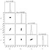 |
Fig. A.1 Results of the emcee MCMC optimization using a single radial power law for the surface density. The panels show one- and two-dimensional projections of the posterior probability functions of the free model parameters. The panels along the diagonal show the marginalized distribution of each of the parameters as histograms; the other panels show the marginalized two-dimensional distributions for each set of two parameters. Contours (barely visible in the tightly constrained probability distributions) and associated greyscale show 0.5, 1, 1.5 and 2σ levels. Best-fit values and error estimates are listed above the panels along the diagonal. |
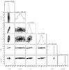 |
Fig. A.2 Results of the emcee MCMC optimization using a broken radial power law for the surface density. Otherwise, the figure is similar to Fig. A.1. No useful constraints on the outer radius Rout are obtained. |
All Tables
All Figures
|
Fig. 1 820 μm (365.5 GHz) continuum of TW Hya based on data set 2011.0.00340.S. We reimaged these data, and obtain a result indistinguishable from (Qi et al. 2013). The image construction employed self-calibration and uniform weighting. The resulting beam size, indicated in the lower left, is |
| In the text | |
|
Fig. 2 Real (black points) and imaginary (red points) parts of the visibilities of project 340.S (previously presented in Qi et al. 2013) in Jy vs deprojected baseline length in kλ. The inset shows the region of 120–420 kλ in greater detail. The dashed black curve shows the recalculated single power-law model of Andrews et al. (2012, their model pC), which fails to reproduce the data on baselines >290 kλ. A much better fit is found for a broken power-law model described in Sect. 3 (solid blue curve). Because both models are symmetric, the imaginary parts of their visibilities are all 0 (not shown). |
| In the text | |
|
Fig. A.1 Results of the emcee MCMC optimization using a single radial power law for the surface density. The panels show one- and two-dimensional projections of the posterior probability functions of the free model parameters. The panels along the diagonal show the marginalized distribution of each of the parameters as histograms; the other panels show the marginalized two-dimensional distributions for each set of two parameters. Contours (barely visible in the tightly constrained probability distributions) and associated greyscale show 0.5, 1, 1.5 and 2σ levels. Best-fit values and error estimates are listed above the panels along the diagonal. |
| In the text | |
|
Fig. A.2 Results of the emcee MCMC optimization using a broken radial power law for the surface density. Otherwise, the figure is similar to Fig. A.1. No useful constraints on the outer radius Rout are obtained. |
| In the text | |
Current usage metrics show cumulative count of Article Views (full-text article views including HTML views, PDF and ePub downloads, according to the available data) and Abstracts Views on Vision4Press platform.
Data correspond to usage on the plateform after 2015. The current usage metrics is available 48-96 hours after online publication and is updated daily on week days.
Initial download of the metrics may take a while.