| Issue |
A&A
Volume 586, February 2016
|
|
|---|---|---|
| Article Number | A155 | |
| Number of page(s) | 33 | |
| Section | Catalogs and data | |
| DOI | https://doi.org/10.1051/0004-6361/201527161 | |
| Published online | 11 February 2016 | |
Absolute magnitudes and phase coefficients of trans-Neptunian objects
1 Observatório Nacional/MCTI, Rua General José Cristino 77, 20921-400 Rio de Janeiro, RJ, Brazil
e-mail: This email address is being protected from spambots. You need JavaScript enabled to view it.
2 Department of Earth and Planetary Sciences, University of Tennessee, Knoxville, TN, 37996, USA
3 Instituto de Astrofísica de Andalucía, CSIC, Apt 3004, 18080 Granada, Spain
4 Lowell Observatory, 1400 W Mars Hill Rd, Flagstaff, 86001 Arizona, USA
Received: 10 August 2015
Accepted: 27 November 2015
Abstract
Context. Accurate measurements of diameters of trans-Neptunian objects (TNOs) are extremely difficult to obtain. Thermal modeling can provide good results, but accurate absolute magnitudes are needed to constrain the thermal models and derive diameters and geometric albedos. The absolute magnitude, HV, is defined as the magnitude of the object reduced to unit helio- and geocentric distances and a zero solar phase angle and is determined using phase curves. Phase coefficients can also be obtained from phase curves. These are related to surface properties, but only few are known.
Aims. Our objective is to measure accurate V-band absolute magnitudes and phase coefficients for a sample of TNOs, many of which have been observed and modeled within the program “TNOs are cool”, which is one of the Herschel Space Observatory key projects.
Methods. We observed 56 objects using the V and R filters. These data, along with those available in the literature, were used to obtain phase curves and measure V-band absolute magnitudes and phase coefficients by assuming a linear trend of the phase curves and considering a magnitude variability that is due to the rotational light-curve.
Results. We obtained 237 new magnitudes for the 56 objects, six of which were without previously reported measurements. Including the data from the literature, we report a total of 110 absolute magnitudes with their respective phase coefficients. The average value of HV is 6.39, bracketed by a minimum of 14.60 and a maximum of −1.12. For the phase coefficients we report a median value of 0.10 mag per degree and a very large dispersion, ranging from −0.88 up to 1.35 mag per degree.
Key words: methods: observational / techniques: photometric / Kuiper belt: general
© ESO, 2016
1. Introduction
The phase curve of a minor body shows how the reduced magnitude1 of the body changes with phase angle. The phase angle, α, is defined as the angle measured at the location of the body that Earth and the Sun subtend. These curves show a complex behavior: for phase angles between 5°and 30° they follow an overall linear trend, while at small angles a departure from linearity often occurs. In 1956 T. Gehrels coined the expression “opposition effect” and attributed it to the sudden increase of brightness at small α shown in the phase curve of asteroid 20 Massalia (Gehrels 1956), although no explanation was offered. Since then, many works have modeled phase curves, with or without opposition effect, analyzing the relationship between these curves and the properties of the surface: particle sizes, scattering properties, albedos, compaction, or composition, either by using astronomical or laboratory data or theoretical modeling (e.g., Hapke 1963; Bowell et al. 1989; Nelson et al. 2000; Shkuratov et al. 2002 and references therein).
In addition to providing information about surface properties, phase curves are also important because by using them, we can measure the absolute magnitude, H, of an airless body. H is defined as the reduced magnitude of an object at α = 0°. Moreover, H is related to the diameter of the body, D, and its geometric albedo p. For magnitudes in the V band, ![Mathematical equation: \begin{equation} \label{diameter} D~[{\rm km}]=1.324\times\frac{10^{(3-H_{V}/5)}}{\sqrt{p_{V}}}\cdot \end{equation}](/articles/aa/full_html/2016/02/aa27161-15/aa27161-15-eq12.png) (1)The first minor bodies with measured phase curves were asteroids (for instance, the aforementioned work by Gehrels in 1956). Today, we know that low-albedo (taxonomic classes D, P, or C) asteroids show lower opposition effect spikes than higher albedo asteroids (S or M asteroids; Belsakya & Shevchenko 2000). Modern technologies have also allowed us to obtain incredible data of a handful of objects. Examples are the recent work on comet 67P/Churyumov-Gerasimenko by Fornasier et al. (2015), which used data from the ROSETTA spacecraft, or huge databases, such as the 250 000 absolute magnitudes of asteroids presented by Vereš et al. (2015) from Pan-STARRS.
(1)The first minor bodies with measured phase curves were asteroids (for instance, the aforementioned work by Gehrels in 1956). Today, we know that low-albedo (taxonomic classes D, P, or C) asteroids show lower opposition effect spikes than higher albedo asteroids (S or M asteroids; Belsakya & Shevchenko 2000). Modern technologies have also allowed us to obtain incredible data of a handful of objects. Examples are the recent work on comet 67P/Churyumov-Gerasimenko by Fornasier et al. (2015), which used data from the ROSETTA spacecraft, or huge databases, such as the 250 000 absolute magnitudes of asteroids presented by Vereš et al. (2015) from Pan-STARRS.
Unfortunately, such data are not yet available for objects farther away in the solar system, with the exception of 134340 Pluto. Therefore, many of the physical characteristic of the trans-Neptunian population, for instance, size, albedo, or density, are still hidden from us because of the limited quality of the information we can currently obtain: visible and/or near-infrared spectroscopy of about 100 objects (Barucci et al. 2011, and references therein), and colors of about 300 (Hainaut et al. 2012) drawn from a known population of more than 1400 objects. Moreover, these data belong to the largest known trans-Neptunian objects (TNOs), the most easily observed ones, or some Centaurs. These last are a population of dynamically unstable objects whose orbits cross those of the giant planets; they are considered to come from the trans-Neptunian region and therefore to be representative of this population. Nevertheless, considerable progress has been made in understanding the dynamical structure of the region, but the bulk of the physical characteristics of the bodies that inhabit it remains poorly determined. Several observational studies conducted in the past years show a vast heterogeneity in physical and chemical properties.
With the objective of enlarging our knowledge of the TNO population, The Herschel open time key program on TNOs and Centaurs: “TNOs are cool” (Müller et al. 2007) was granted with 372.7 h of observation on the Herschel Space Observatory (HSO). The observations are complete with a sample of 130 observed objects. The observed data are fed into thermal models (Müller et al. 2010), where a series of free parameters are fitted; among them are pV and D. These two quantities could be constrained using ground-based data and thus fixing at least one of them in the modeling, which improves the accuracy of the results. Several of the targets observed with Herschel do not have a reliable HV magnitude, which is fundamental to compute D and pV (i.e., small uncertainties in HV mean smaller uncertainties in D and pV).
To supply this, the HSO program “TNOs are cool” needs support observations from ground-based telescopes.
One critical problem that arises when studying phase curves of TNOs is the fact that α can only attain low values for observations made from Earth-based facilities. For comparison: a typical main-belt asteroid can be observed up to 20° or 30°, while a typical TNO can only reach up to 2°. This means that for TNOs, we are observing well within the opposition effect region, which prevents us from using the full power of photometric models. On the other hand, the phase curves are very well approximated by linear functions within this restricted phase angle region (e.g., Sheppard & Jewitt 2002). Some efforts have been made in this direction (see review by Belskaya et al. 2008, or the recent works by Perna et al. 2013; and Böhnhardt et al. 2014), but most of them used limited samples (usually one observation) and assumed average values of the phase coefficients.
With this in mind, we started a survey with various telescopes to obtain V and R magnitudes for several TNOs at as many different phase angles as possible to measure phase curves and through them determine HV. The survey is being carried out in both hemispheres using telescopes at different locations. In the next section we describe the observations and the facilities where the data were obtained. In Sect. 3 we present the results, while their analysis is presented in Sect. 4. The discussion and some conclusions obtained from this work are presented in Sect. 5.
2. Observations and data reduction
The data we present here were collected during several observing runs between September 2011 and July 2015 for well over 40 nights. The instruments and facilities used were the Calar Alto Faint Object Spectrograph at the 2.2 m telescope, CAHA2.2, and the Multi Object Spectrograph for Calar Alto at the 3.5 m telescope, CAHA3.5, of the Calar Alto Observatory2, which is located at the Sierra de Los Filabres (Spain); the Wide Field Camera at the 2.5 m Isaac Newton Telescope (INT), located at the Roque de los Muchachos Observatory3 (Spain); the direct camera at the 1.5 m telescope, OSN, of the Sierra Nevada Observatory4 (Spain); the SOAR Optical Imager at the 4.1 m Southern Astrophysical Research telescope5 located at Cerro Pachón (Chile); the direct camera at the 1 m telescope of the Observatório Astronômico do Sertão de Itaparica6, OASI, Brazil; and the optical imaging component of the Infrared-Optical suite of instruments (IO:O) at the 2.0 m Liverpool telescope, Live, located at the Roque de los Muchachos Observatory7 (Spain). Descriptions of instruments and telescopes can be found at their respective homepages.
We always attempted to observe using the V and R filters sequentially, but in some cases this was not possible, either because of deteriorating weather conditions (i.e., no observation was possible) or because of instrumental or telescope problems. The objects were targeted, whenever possible, at different phase angles, aiming at the widest spread possible. Along with the TNOs we targeted several standard star fields each night (from Landolt 1992; and Clem & Landolt 2013), or they were provided by the observatory, as in the case of the Liverpool telescope. We aimed at observing three different fields at three different airmasses per night to cover the range of airmasses of our main targets.
Most observations were carried out by observing the target during three exposures of 600 s per filter, although in some cases shorter exposures (300 or 400 s) were used to avoid saturation from nearby bright stars or trailing by faster objects (a Centaur can reach up to 2 arcsecs in 10 min). We did not use differential tracking. The combination of the different images allowed us to increase the signal-to-noise ratio while keeping trailing at reasonable values. We found this approach better than tracking at a non-sidereal rate for 1800 s, for instance, because we obtained a better removal of bad pixels, cosmic ray hits, or background sources during stacking of shorter exposures.
Data reduction was performed using standard photometric methods with IRAF. Master bias frames were created from daily files, as well as master flat fields in both filters. Files including TNOs and standard stars fields were bias- and flat-field calibrated. Data from the Liverpool telescope were provided already calibrated. For most of the objects, identification was straightforward by blinking different images or, in the most complicated cases, using Aladin8 (Bonnarel et al. 2000). Instrumental apparent magnitudes were obtained using aperture photometry, for which we selected an aperture typically three times the seeing measured in the images for TNOs and standard stars. Whenever a TNO was too close to another source, either by poor observing timing or by crowded fields, we instead performed aperture correction (see Stetson 1990).
Using the standard stars, we computed extinction coefficients and color terms to correct the magnitudes of the TNOs thus ![Mathematical equation: \begin{equation} m_0=m-\chi[k_1+k_2(v-r)], \end{equation}](/articles/aa/full_html/2016/02/aa27161-15/aa27161-15-eq14.png) (2)where m0 is the apparent instrumental magnitude corrected by extinction (v0 or r0), m is the apparent instrumental magnitude (v or r), χ is the airmass, k1 and k2 are the zeroth- and first-order extinction coefficients, and (v−r) is the apparent instrumental color of the TNO.
(2)where m0 is the apparent instrumental magnitude corrected by extinction (v0 or r0), m is the apparent instrumental magnitude (v or r), χ is the airmass, k1 and k2 are the zeroth- and first-order extinction coefficients, and (v−r) is the apparent instrumental color of the TNO.
Next, we translated m0 into the standard system. The transformation, to order zero, is 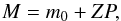 (3)where M is the calibrated magnitude, and ZP is the zero point. We note that because we had many runs in the same telescopes, we computed average extinction coefficients for each site that were used whenever the data did not allow us to compute the night value. The same is true for ZPs. In the particular case of the Liverpool telescope, we used the average extinction coefficient for the Roque de los Muchachos observatory.
Table A.1 lists all observed objects, along with its calibrated V and R magnitudes, the night the object was observed, the heliocentric (r) and geocentric (Δ) distances, and the phase angle (α) at the moment of observation, the telescope used, and a series of notes indicating whether we used average extinction coefficients, average zero points, or if the object had no previously reported data.
The errors in the final magnitudes include (i) the error in the instrumental magnitudes, provided by IRAF (σi); (ii) the error due to atmospheric extintion, estimated as σe = m0−(m−χk1); and the error in the calibration to the standard system, σZP. Therefore 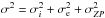 . Whenever aperture correction was performed,
  , where σi1 is the error provided by IRAF within the smaller aperture and σi2 is the error in the aperture correction, computed using the task mkapfile within IRAF.
3. Analysis
In total we obtained 237 new magnitudes for 56 objects, 6 of which did not have any magnitude reported before, to the best of our knowledge. The observed objects span from Centaurs up to detached objects (semi-major axis from 10 to more than 100 AU), while in eccentricity they reach values as high as 0.9. The inclinations are mostly below 40°, with one object at about 80° and one in retrograde orbit (2008 YB3).
At the same time as we acquired our own data, we made an extensive, although not complete, search in the literature of other published V and R magnitudes. We used as our primary reference database the MBOSS 2 article by Hainaut et al. (2012), but we did not take the data directly from their catalog. Instead we took the data from each referenced article to be included in our list. We chose this approach because we need reduced magnitudes (described in Sect. 3.2) to compute the phase curves, which are computed using the heliocentric and geocentric distances at the moment of observation. At the same time, we obtained information regarding the phase angle. Of course we only used data that were reported along with the site and epoch of observation. We obtained the orbital information from JPL-Horizons9. For data of rotational light-curves, i.e., many magnitudes reported for the same night, we computed the average value and its standard deviation to use as input.We finally had more than 1800 individual measurements for over a hundred objects. Each individual measurement corresponds to one observing night or entry. We did not reject any data based on their reported error bars.
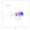 |
Fig. 1 Color−magnitude diagram for the objects in our database. We show in red the objects that have at least one color measured by us, while objects whose data come from the literature alone are shown in blue. The (V−R)⊙ is shown for reference as a horizontal line. |
Before we discuss the results, we stress three important points: (i) we obtained data for 56 objects, but these data alone cannot be used to create phase curves for all the objects, therefore we also consulted the literature. This augmented set of data is called our database. (ii) As can be seen in Eq. (1), we cannot split albedo and diameter using HV alone, therefore whenever we speak about the brightness of an object, we refer exclusively to its magnitude and not to its albedo properties or its size, unless explicitly mentioned. (iii) The magnitudes for the phase curves should be averaged over the rotational period to remove the effect of variability that is due to Δm > 0, which is not the case for individual measurements.
In the following subsections we first describe how we computed the colors for the complete database, and then report how we constructed the phase curves.
3.1. Colors
Because it is a compilation from different sources, our database is very heterogeneous. Some objects have many entries, in a few cases more than fifty, while most have fewer than ten entries (72% of the sample). Not all entries have data obtained with both filters; in some cases, only the V filter was used, while in some others only the R filter magnitude is available. Whenever both magnitudes were available for the same night, we computed (V−R). In this way, many objects have more than one measurement of (V−R). In these cases, we computed a weighted average color, which we took as representative for the object. By doing so, we weighted the most precise values of (V−R) instead of considering possible changes of color with phase angle, which is beyond the scope of the present work.
We show the color−magnitude diagram for all objects in our sample in Fig. 1. If at least one entry for a given object was observed by us, we labeled that object “this work”, while if all observations for a given object were obtained from the literature, the label “literature” was used. The plot has more than 110 points because we also show the colors of objects that did not satisfy our criteria for constructing the phase curve (see below).
Most objects shown in the figure are redder than the Sun, (V−R)⊙ = 0.36. Nevertheless, there are a few bluer objects, (V−R) ≈ 0. The great majority of the objects cluster at V ≈ 23, (V−R) ≈ 0.6. The figure also clearly shows that our observations have a clear cutoff at about V = 22.5, which is due to the size of the telescopes used, with only one object fainter than V = 23: 2003 QA91; this has obvious large error bars.
3.2. Phase curves
The main objective of this work is to compute absolute magnitudes, HV, and phase coefficients, β, of as many objects as possible. These data could be used as complement to the Herschel Space Observatory “TNOs are cool” key project. Several papers have already been published presenting HV of different TNOs (e.g., Sheppard & Jewitt 2002; Rabinowitz et al. 2006, 2007; Perna et al. 2013; Böhnhardt et al. 2014, and others). We do not intend to repeat these works step by step, but to recompute the phase curves and make the most of the increasing amount of data available today. We are aware of the risks that arise as a result of the inhomogeneity of telescopes, instruments, detectors, and epochs. Nevertheless, we consider it important to reanalyze the available data using, if not homogeneous inputs, at least homogeneous techniques.
As mentioned above, we had to deal with the fact that not all entries (i.e., nights of observation for a given object) were complete, in the sense that some objects for a given date were observed only in one filter, V or R. To find a solution for this problem, we decided to construct the individual phase curves using magnitudes measured with the V filter. When V was not available, we used the average color measured above and the R magnitude to obtain V. We decided, for the scope of this work, to not analyze the V and R data separately because we are more interested in obtaining the larger possible quantity of the phase curves. For instance, if we were to use only the V data, without the R data, we would only obtain about 50 phase curves. A similar number of phase curves are obtained when only R data are used, although not necessarily for the same objects.
The next step is to compute the reduced V, whose notation is V(1,1,α), which is the value used in the phase curves. It represents the magnitude of the object if it is located at 1 AU from the Sun and is observed at a distance of 1 AU from Earth.
The reduced magnitude is computed from the values of V and the orbital information as 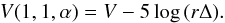 (4)We are now left with a set { V(1,1,α),α } for each object.
For the phase curves we only used data for objects that were observed at least at three different phase angles. We discarded a few objects that had a small coverage in α, which results in unreliable values of HV. We analyzed a total of 110 objects. For objects with no reported light-curve amplitude we assumed Δm = 0 and performed a linear regression to measure HV via 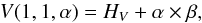 (5)where β is the change of magnitude per degree, also known as phase coefficient. Each V(1,1,α) was weighted by its error, assumed equal to that of the V magnitude, or propagated from the R magnitude and that of the average color, while α was assumed to have a negligible error. By doing so, we obtained HV as the y-intercept and β as the slope of Eq. (5).
We used the linear approach instead of using the full H-G system (Bowell et al. 1989) for simplicity because we do not wish to add any more free parameters that will unnecessarily complicate the interpretation of results. We also made use of the results presented in Belskaya & Shevchenko (2000), mentioned in the Introduction, who showed that the opposition effect, the major departure from linearity of the phase curve, is in fact more conspicuous in moderate-albedo objects (pV> 0.25), which is not the case for most of the known TNOs (e.g., Lellouch et al. 2013; Lacerda et al. 2014).
Some objects do have reported rotational light-curves with non-zero Δm (we here use the data reported in Thirouin et al. 2010, 2012). We note that Δm can cover a range of up to half a magnitude in extreme, but rare, cases. Because we used reduced magnitudes obtained on different nights and mostly individual measurements, we modeled the effect of light-curve variations on the value of V(1,1,α). We proceeded as follows: for an object with Δm ≠ 0 we generated from { V(1,1,α),α } new sets { Vi(1,1,α),α }, with i running from 1 to 10 000, where  (6)randi is a random number drawn from a uniform distribution within −1 and 1. By doing so, and feeding these values into Eq. (5), we compiled a set { HVi,βi }, from where we obtain HV and β as the average over the 10 000 realizations.
In other words, for objects with Δm> 0 we have 10 000 different solutions for Eq. (5). We computed the average of the solutions for HV and β and assumed these values as the most likely result. A graphical representation of the procedure is shown in Fig. 2. The left panel shows the representative phase curve along with the data points and their errors, while the right panel shows a two-dimensional histogram showing the phase-space covered by the 10 000 solutions.
 |
Fig. 2 Example of phase curve of 1996 TL66. Left: scatter plot of V(1,1,α) versus α. The line represents the solution for HV and β as mentioned in the text. Right: density plot showing the phase space of solutions of Eq. (5) when Δm ≠ 0, in gray scale. The effect of the Δm may cause values between 5.0 and 5.5 for HV, while the same is true for β ∈ (0.041,0.706) mag per degree. The continuous lines (red) show the area that contains 68.3, 95.5, and 99.7% of the solutions. |
This method allowed us to explore the solution space, from which we found some interesting results, such as those unexpected cases with β< 0, which we discuss in Sect. 5.
All results are shown in Table A.2. The table reports the observed object, HV and β, the number of points used in the fits, the light-curve amplitude, and the references to the works whose reported magnitudes were used. The phase curves are shown in Figs. A.1−A.110.
4. Results
We measured HV and β for a total of 110 objects. Figure 3 shows the distribution of HV resulting from applying our procedure. The distribution looks bimodal, with the larger peak at HV≈ 7 and a second one at HV≈ 5. Our results cover a range from a minimum of HV= 14.6 (2005 UJ438) up to a maximum of −1.12 for Eris. The average value is 6.39, while the median is 6.58. The distribution of β is shown in Fig. 4. The average value is 0.09 mag per degree, while the median is 0.10 mag per degree, with a minimum of −0.88 mag per degree for 2003 GH55 and a maximum of 1.35 mag per degree for 2004 GV9. Almost 60% of the values fall within 0.01 and 0.23 mag per degree.
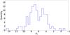 |
Fig. 3 Histogram showing the HV distribution. |
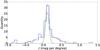 |
Fig. 4 Histogram showing the β distribution. The dashed black line is the better fit to the distribution, modeled as the sum of two Gaussian distributions (see text). Each individual Gaussian distribution is shown as continuous green and dotted red lines. |
Curiously, the distribution shown in Fig. 4 seems to be the combination of two different distributions, one wide and shallow, and a second one sharp and tall. To test this possibility, we assumed that the distribution could be fitted by a sum of two Gaussian distributions 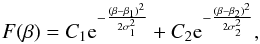 where Ci, βi, and σi are free parameters.
We ran a minimization script from python (scipy.optimize.leastsq) to obtain all six free parameters: C1 = 6.8, σ1 = 0.27 mag per degree, β1 = 0.10 mag per degree, and C2 = 26.2, σ2 = 0.05 mag per degree, β2 = 0.11 mag per degree. The best-fitting F(β) is shown in Fig. 4, along with the two components. The two-Gaussian model describes the distribution of β very well, both with similar modes but different widths. We return to this model in the Discussion.
Next, we compared our results with those of a few selected works: Rabinowitz et al. (2007), Perna et al. (2013), and Böhnhardt et al. (2014); and then we searched for correlations among our results (HV, colors, β), orbital elements (semi-major axis, eccentricity, inclination), the absolute magnitudes used in the “TNOs are cool” Herschel Space Observatory key project and their measured geometric albedos, and the light-curve amplitude Δm. Orbital elements for each object were obtained from the Lowell Observatory10.
4.1. Comparison with selected works
On one hand, we selected Rabinowitz et al. (2007, Ra07) because it has the densest phase curves reported for 25 outer solar system objects, while on the other hand, Perna et al. (2013, Pe13) and Böhnhardt et al. (2014, Bo14) presented results in support for the HSO “TNOs are cool” key project. The three works analyze their data following different criteria: Ra07 observed each target on many occasions, even attempting to obtain rotational properties. If a rotational light-curve could be determined, the data were corrected removing the short-term variability, the remaining data were then rebinned in α, and then the phase curves were constructed. Pe13, using less dense data, computed phase curves for a few objects, while average values of β were assumed for objects without enough data . Bo14 only used average values of β.
We report in Table A.3 the comparison between our results and those from Ra07, Pe13, and Bo14. We note that our phase curves include the data reported in these three works.
Overall, the four works agree very well. Nevertheless, some values differ beyond three sigma. For clarity we report these differences here (shown in boldface in Table A.3). With Ra07 Makemake (HV and β) and Sedna (HV); with Pe13 2005 UJ438 (HV) and Varda (HV); with Bo14 2003 GH55, 2004 PG115, and Okyrhoe. In this last case the differences are only in HV because these authors did not compute the phase curve, but instead used average values of β to obtain absolute magnitudes. Moreover, the errors in our data are somewhat larger than those in Ra07, Pe13, and Bo14. We return to this issue in the discussion.
4.2. Correlations
We searched for possible correlations among pairs of variables. We define here a variable as any given set of quantities representing the population, for instance, the variable β is the set of phase coefficients of the TNOs sample. The correlations were explored using a Spearman test, which has the advantage of being non-parametric because it relies on ordering the data according to rank and running a linear regression through those ranks. The test returned two values. The first one, rs, gives the level of correlation of the tested variables, | rs | ≈ 1 indicates correlated quantities, while | rs | → 0 indicates uncorrelated data. The second value is Prs which indicates the probability of two variables to be uncorrelated, in practical terms, the closer Prs is to zero, the more likely becomes the result provided by rs.
One disadvantage of the Spearman test is that it does not consider the errors in the variables. To overcome this problem, we proceeded as follows: we tried to find the correlation among a set { xj,yj }, where each quantity xj (yj) has an error of σxj (σyj), j running from 1 up to N. Then we created 10,000 correlations by creating new sets { xji,yji }, where xji = xj + randi × σxj, likewise for yj. In this case, randi is a random number drawn from a normal distribution in [−1,1]. The random number in xj is not necessarily the same as in yj.
After performing the 10 000 correlations, we had a set { rsi,Prsi }, which is displayed in the form of density plots to show the likelihood of the correlation to hold against the error bars. All relevant results are displayed in Figs. 5−11. Table 1 shows the result of the correlation tests: the first column shows the variables tested, the second and third column show the nominal values of rs and Prs (those where the errors were not accounted for), while the last column reports our interpretation of the density plots of whether the correlation exists or not.
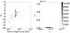 |
Fig. 5 Left: scatter plot of HV vs. semi-major axis. Right: outcome of the 10 000 realizations in form of a two-dimensional histogram in rs and Prs which shows the phase space where the solutions lie. In a few cases it is relatively clear that a correlation might exists, while in some other cases large excursions are seen, which indicate that a false correlation could arise in the case of large errors. |
Correlations.
For the scope of the present work we decided not to separate our sample into the subpopulations that appear among Centaurs and TNOs because dividing a sample of 110 objects into smaller samples will only decrease the statistical significance of any possible result. Furthermore, should any real difference arise among any subgroup, this would clearly be seen in any of the tests proposed here, for instance, the fact that no large Centaurs are known, or that the so-called cold classic TNO have low inclinations and tend to be smaller in size than other subpopulations of TNOs. Below we report the most interesting findings of the search for correlations. Thereafter, we discuss some individual cases that showed interesting or anomalous behavior.
HV vs. semi-major axis: Fig. 5 shows the correlation between absolute magnitude and semi-major axis. This correlation is due to observational bias and accounts for the lack of faint objects detected at large heliocentric distances, while no bright Centaur (we loosely define a Centaur as an object with a semi-major axis below 30 AU) is known to exist.
HV(ours) vs. HV(HSO): in this case we compared our computed magnitudes with those used by the Herschel Space Observatory “TNOs are cool” key project. The correlation is close to 1 (Fig. 6), although it is possible to see a small departure at the faint end with two objects with significantly smaller HV, they are (250112) 2002 KY14 (HV= 11.808 ± 0.763, Fig. A.50) and (145486) 2005 UJ438 (HV= 14.602 ± 0.617, Fig. A.78). In the first case we revised the data without finding any evident problem and we trust the value to be correct, while in the second case some care should be taken because the minimum value of the phase angle is about 5.8° , leaving most of the phase curve undersampled, which might affect the value of β.
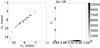 |
Fig. 6 Left: scatter plot of HV as measured by us vs. (ours). HV as used within the “TNO’s are cool” program (HSO). Right: two-dimensional histogram showing the most likely correlations. |
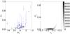 |
Fig. 7 Left: scatter plot of HV vs. the geometric albedo measured by the “TNOs are cool” program. Right: two-dimensional histogram showing the most likely correlations. |
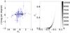 |
Fig. 8 Left: scatter plot of β vs. HV. Right: two-dimensional histogram showing the most likely correlations. |
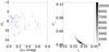 |
Fig. 9 Left: scatter plot of HV vs. Δm. Right: Two-dimensional histogram showing the most likely correlations. |
For the sake of comparison, we fitted a linear function to the data according to HV(ours)= a + b × HV(HSO), obtaining b = 1.06 ± 0.03 and a = −0.27 ± 0.17. This indicates that although HV(ours) are very similar to HV(HSO), they are not identical. This difference between our HV and those used by the “TNOs are cool” team probably arises because some of theirs were computed using single observations and assuming an average β.
HV vs.pV: Fig. 7 shows a correlation between the absolute magnitude and the geometric albedo: the brigher the object, the larger the albedo. This probably reflects the fact that brighter objects tend to be the larger in size as well and are therefore able to retain part of the original volatiles, more reflective species, that smaller objects cannot.
βvs. HV: HV seems to have a weak anticorrelation with β, indicating that brighter objects have larger positive slopes than fainter ones. From Fig. 8 one interesting detail arises: there are a few objects with β< 0 (see also Fig. 4), even considering the error bars and light-curve amplitude (see Table A.2). This issue deserves further study and observations. According to the density map, the weak correlation seems quite consistent within the errors in HV and β.
HV vs.Δm: there is a weak correlation between absolute magnitude and Δm, which indicates that brighter objects tend to have lower Δm. Interestingly, among the faint object (fainter than HV= 10) no large (> 0.25) amplitudes are found (Fig. 9). We recall that although they are faint objects, they are usually in the range 50 to 100 km11.
Duffard et al. (2009) presented a similar value for this correlation. Using their results (their Fig. 6), we also see that objects with densities lower than 0.7 g cm-3 are unlikely in hydrostatic equilibrium and therefore could have large Δm, which is not reflected in our Fig. 9. These density correspond to ≈ 400 km (from Fig. S7 in Ortiz et al. 2012), which is roughly HV≈ 5.4. Brighter, possibly larger, objects are in hydrostatic equilibrium and their shapes are better described by Mclaurin spheroids whose Δm are harder to measure because they are symmetric around the minor axis.
HV vs. eccentricity and inclination: there are two curious cases (Figs. 10 and 11). The first one, HV vs. eccentricity, indicates that fainter objects tend to have higher eccentricities. This is an observational bias because faint objects are more easily observed close to perihelion, favoring objects with high eccentricties. The second one, HV vs. inclination, also shows a weak tendency of fainter objects having smaller inclinations. This might be reflecting the known fact that two supopulations are found in the so-called classical trans-Neptunian belt, which are distunguished as a hot and a cold population (from dynamical considerations). The cold, low-inclination population does not have objects as large as the hot, high-inclination, population. Although both tendencies seem significant over the 2-sigma level (> 95.5%), only one seems closer to be a correlation with | rs | > 0.3.
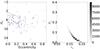 |
Fig. 10 Left: scatter plot of HV vs. eccentricity. Right: two-dimensional histogram showing the most likely correlations. |
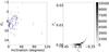 |
Fig. 11 Left: scatter plot of HV vs. inclination. Right: two-dimensional histogram showing the most likely correlations. |
Other results:
none of the other pairs of variables explored show any significant correlation, therefore their plots are not reported.
Interesting objects:
in this paragraph we describe some objects that deserve more discussion.
2060 Chiron: Meech & Belton (1989) detected a coma surrounding Chiron; this result probably influenced the interpretation of latter stellar occultations results (e.g., Bus et al. 1996) that detected secondary events which were associated with jets of material ejected from the surface. A recent reanalysis of all stellar occultation data, along with new photometric data, suggests that Chiron possesses a ring system (Ortiz et al. 2015). These two phenomena, cometary-like activity and the possible ring system, affect the photometric data obtained from Chiron, including the way the photometric measurements are performed, thus increasing the scattering in the phase curve (Fig. A.90).
10199 Chariklo: Braga-Ribas et al. (2014) detected a ring system around Chariklo using data from a stellar occultation. This result helped to interpret long-term changes in photometric and spectroscopic data (Duffard et al. 2014), such as the secular variation in reduced magnitude (Belskaya et al. 2010) and the disappearance of a water-ice absorption feature in its near-infrared spectrum (Guilbert et al. 2009). As for Chiron, the phase curve of Chariklo does not follow a linear trend (Fig. A.89).
Bright objects: those with HV brighter than 3 have β between 0.11 and 0.27 mag per degree (Figs. A.80, A.94, A.98, A.100, A.103, and A.105). Spectroscopically it is known that these objects (2007 OR10, Eris, Makemake, Orcus, Quaoar, and Sedna) are very different; Eris and Makemake display methane ice absorption features, while Orcus, Quaoar, and 2007 OR10 show water ice and probably some hydrocarbons. Therefore, particle size or compaction could play a more important role than composition on the phase curves.
5. Discussion and conclusions
We have observed 56 objects, six of them with no previously reported magnitudes in the literature, to the best of our knowledge. We combined these new V and R magnitudes with an extensive bibliographic survey to compute absolute magnitudes and phase coefficients. In total we report HV and β for 110 objects. Some of these objects already had reported phase curves, nevertheless, it is important to include new data, always keeping in mind that we combined data from different apparitions for the same object and that surface conditions might have changed between observations.
Regarding the distribution of β, Fig. 4 clearly shows a quasi-symmetric distribution. The maximum and mode coincide to the second decimal place with the average and median values: 0.10 mag per degree. We tested the hypothesis of having a two-population distribution by assuming that each population could be described by a Gaussian function. The fit to the data is quite good, but does this indicate the existence of two real subpopulations? One possible explanation regards the quality of the data: There might be a high-quality subsample cluster with a mode of β2 = 0.11 mag per degree within a sharp distribution, while the low-quality data are more spread out, but with a very similar mode (β2 = 0.10 mag per degree). This would consider as high-quality data those with small errors, precise β, and with (at least) an estimate of Δm. Unfortunately, this is not strictly the case because some of these objects fall within the wings of the wide and shallow distribution. Therefore, even if it is very tempting, we cannot use the sharp distribution as representative of the whole population because we might introduce undesired biases in the results. Moreover, most of the objects fall within the wide distribution, 59%, while 41% fall within the sharp one.
It is clear that there is not one representative value of β for the whole population. Therefore, the use of average values of β to compute HV should be regarded with caution. The phase coefficients range from −0.88 up to 1.35 mag per degree. On the extreme positive side, the two objects (1996 GQ21, Fig. A.11; and 2004 GV9, Fig. A.68) have large associated errors. Among the extreme negative values are six objects (1998 KG62, Fig. A.25; 1998 UR43, Fig. A.28; 2002 GP32, Fig. A.47; 2003 GH55, Fig. A.61; 2005 UJ438, Fig. A.78; and Varda, Fig. A.109) with β< 0, even considering three times the error. Most of these cases are objects whose data are sparse and with few points. Two of them, UJ438 and Varda, have an estimated light-curve amplitude, while the rest has no reported value to the best of our knowledge.
We are not aware of any physical mechanism that could explain a β< 0 using scattering models. There are some components of the light that could be negative, such as the incoherent second scattering order (Fig. 21 in Shkuratov et al. 2002), which is nonetheless non-dominant, especially for the low values of α that we can observe TNOs with.
These extremes values, either positive or negative, could be due to as yet undetected phenomena, such as poorly determined rotational modulation, ring systems, or cometary-like activity. They deserve more observations.
Some phase curves clearly do not follow a linear trend. Those of Chiron and Chariklo, in fact, do not follow any particular trend at all. It is convenient to bear in mind that the photometric models for understanding the photometric behavior of phase curves were made for objects with nothing else than their bare surface to reflect, scatter, or absorb photons. In the case of these possibly ringed systems the reflected light detected on Earth depends not only on the scattering properties of the material covering Chiron or Chariklo, but also on the particles in the rings and the geometry of the system. With this in mind, we propose that one criterion to seek candidates that bear ring systems is to search for this “non-linear” behavior of the phase curve. As examples, based on the dispersion seen in their phase curves, we propose that 1996 RQ20 (Fig. A.12), 1998 SN165 (Fig. A.27), or 2004 UX10 (Fig. A.71) might be candidates for further studies, among other objects.
The correlations were discussed in their respective paragraphs. Overall, some of them are associated with observational biases (HV and semi-major axis; HV and eccentricity), others can be interpreted in terms of known properties of the TNO region (HV and inclination), while the rest can be considered as weak or non-existing and deserving more data, especially going deeper into the faint end of the population. We do not confirm the proposed anticorrelation between albedo and phase coefficient (see Belskaya et al. 2008 and references therein). One special note about the anticorrelation found between HV and pV: it would seem that the correlation is driven principally by the brighter objects. We ran the same test discarding objects brighter than 3 and those associated with the Haumea dynamical group because they form a group that stands apart with particular surface properties, and the relation still holds, rs = −0.356,Prs = 0.0092. Although the correlation does become weaker, without reaching a 3−σ level, there seems to exists a trend of brighter objects to have larger geometric albedos. An in-depth physical explanation remains yet to be formulated.
Finally, the errors reported in HV are in some cases larger than in previous works. This reflects the heterogeneity of the sample, how the effect of the rotational variability is considered, and the weighting of the data while performing the linear fits. For instance, we note that all of the objects with σHV> 0.1 mag have either fewer than ten data points or Δm> 0.1 mag. Taking this into consideration, our results are more accurate than, although not as precise as, previous works and probably more realistic, with the exception of the strategy followed by Rabinowitz et al. (2007).
This work represents the first release of data taken at seven different telescopes in six observatories between late 2011 and mid-2015, which represents a large effort. It is important to mention that more observations are ongoing.
The observed standard magnitude normalized to the distance of the Sun and Earth.
Acknowledgments
Based in part on observations collected at the German-Spanish Astronomical Center, Calar Alto, operated jointly by Max-Planck-Institut für Astronomie and Instituto de Astrofísica de Andalucía (CSIC). Based in part on observations made with the Isaac Newton Telescope operated on the island of La Palma by the Isaac Newton Group in the Spanish Observatorio del Roque de los Muchachos of the Instituto de Astrofísica de Canarias. Partially based on data obtained with the 1.5 m telescope, which is operated by the Instituto de Astrofísica de Andalucía at the Sierra Nevada Observatory. Partially based on observations obtained at the Southern Astrophysical Research (SOAR) telescope, which is a joint project of the Ministério da Ciência, Tecnologia, e Inovação (MCTI) da República Federativa do Brasil, the U.S. National Optical Astronomy Observatory (NOAO), the University of North Carolina at Chapel Hill (UNC), and Michigan State University (MSU). Based in part on observations made at the Observatório Astronômico do Sertão de Itaparica operated by the Observatório Nacional/MCTI, Brazil. Partially based on observations made with the Liverpool Telescope operated on the island of La Palma by Liverpool John Moores University in the Spanish Observatorio del Roque de los Muchachos of the Instituto de Astrofísica de Canarias with financial support from the UK Science and Technology Facilities Council. A.A.C. acknowledges support through diverse grants to FAPERJ and CNPq. J.L.O. acknowledges support from the Spanish Mineco grant AYA-2011-30106-CO2-O1, from FEDER funds and from the Proyecto de Excelencia de la Junta de Andalucía, J.A. 2012-FQM1776. R.D. acknowledges the support of MINECO for his Ramón y Cajal Contract. The authors would like to thank Y. Jiménez-Teja for technical support and P.H. Hasselmann for helpful discussions regarding phase curves. We are grateful to O. Hainaut, whose comments helped us to improve the quality of this manuscript.
References
- Barucci, M. A., Romon, J., Doressoundiram, A., et al. 2000, AJ, 120, 496 [NASA ADS] [CrossRef] [Google Scholar]
- Barucci, M. A., Böhnhardt, H., Dotto, E., et al. 2002, A&A, 392, 335 [NASA ADS] [CrossRef] [EDP Sciences] [Google Scholar]
- Barucci, M. A., Cruikshank, D. P., Dotto, E., et al. 2005, A&A, 439, L1 [NASA ADS] [CrossRef] [EDP Sciences] [Google Scholar]
- Barucci, M. A., Alvarez-Candal, A., Merlin, F., et al. 2011, Icarus, 214, 297 [NASA ADS] [CrossRef] [Google Scholar]
- Belskaya, I., & Shevchenko, V. 2000, Icarus, 147, 94 [NASA ADS] [CrossRef] [Google Scholar]
- Belskaya, I. N., Levasseur-Regourd, A.-C., Shkuratov, Y. G., et al. 2008, in The Solar System Beyond Neptune, eds. M. A. Barucci, H. Boehnhardt, D. P. Cruikshank, et al. (Tucson: Univ. of Arizona Press), 115 [Google Scholar]
- Belskaya, I. N., Bagnulo, S., Barucci, M. A., et al. 2010, Icarus, 210, 472 [NASA ADS] [CrossRef] [Google Scholar]
- Bonnarel, F., Fernique, P., Bienaymé, O., et al. 2000, A&ASS, 143, 33 [NASA ADS] [CrossRef] [EDP Sciences] [Google Scholar]
- Böhnhardt, H., Tozzi, G.-P., Birkle, K., et al. 2001, A&A, 378, 653 [NASA ADS] [CrossRef] [EDP Sciences] [Google Scholar]
- Böhnhardt, H., Delsanti, A., Barucci, M. A., et al. 2002, A&A, 395, 297 [NASA ADS] [CrossRef] [EDP Sciences] [Google Scholar]
- Böhnhardt, H., Schulz, D., Protopapa, S., & Götz, C. 2014, Earth Moon Planet, 114, 35 [Google Scholar]
- Bowell, E., Hapke, B., Domingue, D., et al. 1989, in Asteroids II, eds. R. P. Binzel, T. Gehrels, & M. Shapely Matthews (Tucson: Univ. of Arizona Press), 524 [Google Scholar]
- Braga-Ribas, F., Sicardy, B., Ortiz, J. L., et al. 2014, Nature, 508, 72 [NASA ADS] [CrossRef] [Google Scholar]
- Brown, W. R., & Luu, J. X. 1997, Icarus, 126, 218 [NASA ADS] [CrossRef] [Google Scholar]
- Buie, M. W., & Bus, S. J. 1992, Icarus, 100, 288 [NASA ADS] [CrossRef] [Google Scholar]
- Bus, S. J., Buie, M. W., Schleicher, D. G., et al. 1996, Icarus, 123, 478 [NASA ADS] [CrossRef] [Google Scholar]
- Carraro, G., Maris, M., Bertin, D., et al. 2006, A&A, 460, L39 [NASA ADS] [CrossRef] [EDP Sciences] [Google Scholar]
- Clem, J. L., & Landolt, A. U. 2013, AJ, 146, 88 [NASA ADS] [CrossRef] [Google Scholar]
- Davies, J. K., Green, S., McBride, N., et al. 2000, Icarus, 146, 253 [NASA ADS] [CrossRef] [Google Scholar]
- Davis, D. R., & Farinella, P. 1997, Icarus, 125, 50 [NASA ADS] [CrossRef] [Google Scholar]
- de Bergh, C., Delsanti, A., Tozzi, G. P., et al. 2005, A&A, 437, 1115 [NASA ADS] [CrossRef] [EDP Sciences] [Google Scholar]
- Delsanti, A., Böhnhardt, H., Barrera, L, et al. 2001, A&A, 380, 347 [NASA ADS] [CrossRef] [EDP Sciences] [Google Scholar]
- DeMeo, F., Fornasier, S., Barucci, M. A., et al. 2009, A&A, 493, 283 [NASA ADS] [CrossRef] [EDP Sciences] [Google Scholar]
- Doressoundiram, A., Barucci, M. A., Romon, J., et al. 2001, Icarus, 144, 277 [NASA ADS] [CrossRef] [Google Scholar]
- Doressoundiram, A., Peixinho, N., de Bergh, C., et al. 2002, ApJ, 124, 2279 [Google Scholar]
- Doressoundiram, A., Peixinho, N., Doucet, C., et al. 2005, Icarus, 174, 90 [NASA ADS] [CrossRef] [Google Scholar]
- Dotto, E., Barucci, M. A., Böhnhardt, H., et al. 2003, Icarus, 162, 408 [NASA ADS] [CrossRef] [Google Scholar]
- Duffard, R., Lazzaro, D., Pinto, S., et al. 2002, Icarus, 160, 44 [NASA ADS] [CrossRef] [Google Scholar]
- Duffard, R., Ortiz, J. L., Thirouin, A., et al. 2009, A&A, 505, 1283 [NASA ADS] [CrossRef] [EDP Sciences] [Google Scholar]
- Duffard, R., Pinilla-Alonso, N., Ortiz, J. L., et al. 2014, A&A, 568, A79 [NASA ADS] [CrossRef] [EDP Sciences] [Google Scholar]
- Farnham, T. L., & Davies, J. K. 2003, Icarus, 164, 418 [NASA ADS] [CrossRef] [Google Scholar]
- Ferrin, I., Rabinowitz, D., Schaefer, B., et al. 2001, ApJ, 548, L243 [Google Scholar]
- Fornasier, S., Doressoundiram, A., Tozzi, G. P., et al. 2004, A&A, 421, 353 [NASA ADS] [CrossRef] [EDP Sciences] [Google Scholar]
- Fornasier, S., Lazzaro, D., Alvarez-Candal, A., et al. 2014, A&A, 568, L11 [NASA ADS] [CrossRef] [EDP Sciences] [Google Scholar]
- Fornasier, S., Hasselmann, P. H., Barucci, M. A., et al. 2015, A&A, 583, A30 [NASA ADS] [CrossRef] [EDP Sciences] [Google Scholar]
- Gehrels, T. 1956, ApJ, 123, 331 [NASA ADS] [CrossRef] [Google Scholar]
- Gil-Hutton, R., & Licandro, J. 2001, Icarus, 152, 246 [NASA ADS] [CrossRef] [Google Scholar]
- Guilbert, A., Barucci, M. A., Brunetto, R., et al. 2009, A&A, 501, 777 [NASA ADS] [CrossRef] [EDP Sciences] [Google Scholar]
- Hainaut, O. R., Böhnhardt, H., & Protopapa, S. 2012, A&A, 546, A115 [NASA ADS] [CrossRef] [EDP Sciences] [Google Scholar]
- Hapke, B. 1963, JGR, 68, 4571 [NASA ADS] [CrossRef] [Google Scholar]
- Jewitt, D. C. 2002, AJ, 123, 1039 [NASA ADS] [CrossRef] [Google Scholar]
- Jewitt, D., & Luu, J. 1993, Nature, 362, 730 [NASA ADS] [CrossRef] [Google Scholar]
- Jewitt, D., & Luu, J. 1998, AJ, 115, 1667 [NASA ADS] [CrossRef] [Google Scholar]
- Jewitt, D., & Luu, J. 2001, AJ, 122, 2099 [NASA ADS] [CrossRef] [Google Scholar]
- Jewitt, D. C., & Sheppard, S. S. 2002, AJ, 123, 2110 [NASA ADS] [CrossRef] [Google Scholar]
- Lacerda, P., Fornasier, S., Lellouch, E., et al. 2014, ApJ, 793, L2 [NASA ADS] [CrossRef] [Google Scholar]
- Lagerkvist, C.-I., Magnusson, P. 1990, A&ASS, 86, 119 [NASA ADS] [Google Scholar]
- Landolt, A. U. 1992, AJ, 104, 340 [NASA ADS] [CrossRef] [Google Scholar]
- Lellouch, E., Santos-Sanz, P., Lacerda, P., et al. 2013, A&A, 557, A60 [NASA ADS] [CrossRef] [EDP Sciences] [Google Scholar]
- McBride, N., Davies, J. K., Green, S. F., et al. 1999, MNRAS, 306, 799 [NASA ADS] [CrossRef] [Google Scholar]
- McBride, N., Green, S. F., Davies, J. K., et al. 2003, Icarus, 161, 501 [NASA ADS] [CrossRef] [Google Scholar]
- Meech, K. J., & Belton, M. J. S. 1989, IAU Circ. 4770, 1 [Google Scholar]
- Mueller, B. E. A., Tholen, D. J., Hartmann, W. K., et al. 1992, Icarus, 97, 150 [NASA ADS] [CrossRef] [Google Scholar]
- Müller, T. G., Lellouch, E., Böhnhardt, H., et al. 2007, Earth Moon Planets, 105, 209 [Google Scholar]
- Müller, T. G., Lellouch, E., Stansberry, J., et al. 2010, A&A, 518, A146 [Google Scholar]
- Nelson, R. M., Hapke, B. W., Smythe, W. D., et al. 2000, Icarus, 147, 545 [NASA ADS] [CrossRef] [Google Scholar]
- Ortiz, J. L., Sota, A., Moreno, R., et al. 2004, A&A, 420, 383 [NASA ADS] [CrossRef] [EDP Sciences] [Google Scholar]
- Ortiz, J. L., Sicardy, B., Braga-Ribas, F., et al. 2012, Nature, 491, 566 [NASA ADS] [CrossRef] [Google Scholar]
- Ortiz, J. L., Duffard, R., Pinilla-Alonso, N., et al. 2015, A&A, 576, A18 [NASA ADS] [CrossRef] [EDP Sciences] [Google Scholar]
- Peixinho, N., Lacerda, P., Ortiz, J. L., et al. 2001, A&A, 371, 753 [NASA ADS] [CrossRef] [EDP Sciences] [Google Scholar]
- Peixinho, N., Böhnhardt, H., Belskaya, I., et al. 2004, Icarus, 170, 153 [NASA ADS] [CrossRef] [Google Scholar]
- Peixinho, N., Delsanti, A., Guilbert-Lepoutre, A., et al. 2012, A&A, 546, A86 [NASA ADS] [CrossRef] [EDP Sciences] [Google Scholar]
- Perna, D., Barucci, M. A., Fornasier, S., et al. 2010, A&A, 510, A53 [NASA ADS] [CrossRef] [EDP Sciences] [Google Scholar]
- Perna, D., Dotto, E., Barucci, M. A., et al. 2013, A&A, 555, A49 [NASA ADS] [CrossRef] [EDP Sciences] [Google Scholar]
- Pinilla-Alonso, N., Alvarez-Candal, A., Melita, M., et al. 2013, A&A 550, A13 [Google Scholar]
- Rabinowitz, D. K., Barkume, K., Brown, M. E., et al. 2006, ApJ, 639, 1238 [NASA ADS] [CrossRef] [Google Scholar]
- Rabinowitz, D. L., Schaffer, B. E., & Tourtellotte, W. 2007, AJ, 133, 26 [NASA ADS] [CrossRef] [Google Scholar]
- Romanishin, W., & Tegler, S. C. 1999, Nature, 398, 129 [NASA ADS] [CrossRef] [Google Scholar]
- Romanishin, W., Tegler, S. C., Levine, J., et al. 1997, AJ, 113, 1893 [NASA ADS] [CrossRef] [Google Scholar]
- Romanishin, W., Tegler, S. C., Consolmagno, G. J. 2010, AJ, 140, 29 [NASA ADS] [CrossRef] [Google Scholar]
- Romon-Martin, J., Barucci, M. A., de Bergh, C., et al. 2002, Icarus, 160, 59 [NASA ADS] [CrossRef] [Google Scholar]
- Santos-Sanz, P., Ortiz, J. L., Barrera, L., et al. 2009, A&A, 494, 693 [NASA ADS] [CrossRef] [EDP Sciences] [Google Scholar]
- Schaefer, B. E., & Rabinowitz, D. L. 2002, Icarus, 160, 52 [NASA ADS] [CrossRef] [Google Scholar]
- Schaller, E., & Brown, M. 2007, ApJ, 659, L61 [NASA ADS] [CrossRef] [Google Scholar]
- Sheppard, S. S. 2010, AJ, 139, 1394 [NASA ADS] [CrossRef] [PubMed] [Google Scholar]
- Sheppard, S. S., & Jewitt, D. C. 2002, AJ, 124, 1757 [NASA ADS] [CrossRef] [Google Scholar]
- Shkuratov, Y., Ovcharenko, A., Zubko, E., et al. 2002, Icarus, 159, 396 [NASA ADS] [CrossRef] [Google Scholar]
- Snodgrass, C., Carry, B., Dumas, C., et al. 2010, A&A, 511, A72 [NASA ADS] [CrossRef] [EDP Sciences] [Google Scholar]
- Stetson, P. B. 1990, PASP, 102, 932 [NASA ADS] [CrossRef] [Google Scholar]
- Tegler, S. C., & Romanishin, W. 1997, Icarus, 126, 212 [NASA ADS] [CrossRef] [Google Scholar]
- Tegler, S. C., & Romanishin, W. 2000, Nature, 407, 979 [NASA ADS] [CrossRef] [PubMed] [Google Scholar]
- Tegler, S. C., & Romanishin, W. 2003, Icarus, 161, 181 [NASA ADS] [CrossRef] [Google Scholar]
- Tegler, S. C., Romanishin, W., Stone, A., et al. 1997, AJ, 114, 1230 [NASA ADS] [CrossRef] [Google Scholar]
- Tegler, S. C., Romanishin, W., & Consolmagno, G. J. 2003, ApJ, 599, L49 [NASA ADS] [CrossRef] [Google Scholar]
- Thirouin, A., Ortiz, J. L., Duffard, R., et al. 2010, A&A, 522, A93 [NASA ADS] [CrossRef] [EDP Sciences] [Google Scholar]
- Thirouin, A., Ortiz, J. L., Campo-Bagatin, A., et al. 2012, MNRAS, 424, 3156 [NASA ADS] [CrossRef] [Google Scholar]
- Vereš, P., Jedicke, R., Fitzsimmons, A., et al. 2015, Icarus, 261, 34 [NASA ADS] [CrossRef] [Google Scholar]
Appendix A: Additional tables and figures
Observations.
Absolute magnitudes.
Comparison between the values of HV and β from this work with those from three selected references.
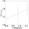 |
Fig. A.1 Phase curve of 15 760 1992 QB1. The continuous line indicate the best fit to Eq. (5) resulting in HV= 7.839 ± 0.097, β = (−0.193 ± 0.132) mag per degree. |
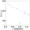 |
Fig. A.2 Phase curve of 15 788 1993 SB. The continuous line indicate the best fit to Eq. (5) resulting in HV= 7.995 ± 0.059, β = (0.374 ± 0.066) mag per degree. |
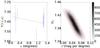 |
Fig. A.3 Left: phase curve of 15 789 1993 SC. The continuous line indicate the best fit to Eq. (5) resulting in HV= 7.393 ± 0.020, β = (0.050 ± 0.017) mag per degree. Right: density plot showing the phase space of solutions of Eq. (5) for Δm = 0.04, in gray scale. The continuous lines show the area that contain 68.3, 95.5, and 99.7% of the solutions. |
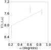 |
Fig. A.4 Phase curve of 1994 EV3. The continuous line indicate the best fit to Eq. (5) resulting in HV= 8.183 ± 0.247, β = (−0.803 ± 0.329) mag per degree. |
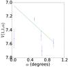 |
Fig. A.5 Phase curve of 16 684 1994 JQ1. The continuous line indicate the best fit to Eq. (5) resulting in HV= 7.031 ± 0.078, β = (0.570 ± 0.125) mag per degree. |
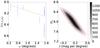 |
Fig. A.6 Left: phase curve of 15 820 1994 TB. The continuous line indicate the best fit to Eq. (5) resulting in HV= 8.017 ± 0.226, β = (0.133 ± 0.152) mag per degree. Right: density plot showing the phase space of solutions of Eq. (5) for Δm = 0.34, in gray scale. The continuous lines show the area that contain 68.3, 95.5, and 99.7% of the solutions. |
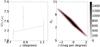 |
Fig. A.7 Left: phase curve of 19 255 1994 VK8. The continuous line indicate the best fit to Eq. (5) resulting in HV= 7.840 ± 0.923, β = (−0.173 ± 0.976) mag per degree. Right: density plot showing the phase space of solutions of Eq. (5) for Δm = 0.42, in gray scale. The continuous lines show the area that contain 68.3, 95.5, and 99.7% of the solutions. |
 |
Fig. A.8 Phase curve of 1995 HM5. The continuous line indicate the best fit to Eq. (5) resulting in HV= 8.315 ± 0.100, β = (0.037 ± 0.074) mag per degree. |
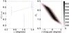 |
Fig. A.9 Left: phase curve of 32 929 1995 QY9. The continuous line indicate the best fit to Eq. (5) resulting in HV= 8.136 ± 0.515, β = (−0.108 ± 0.459) mag per degree. Right: density plot showing the phase space of solutions of Eq. (5) for Δm = 0.60, in gray scale. The continuous lines show the area that contain 68.3, 95.5, and 99.7% of the solutions. |
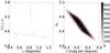 |
Fig. A.10 Left: phase curve of 24 835 1995 SM55. The continuous line indicate the best fit to Eq. (5) resulting in HV= 4.584 ± 0.178, β = (0.139 ± 0.198) mag per degree. Right: density plot showing the phase space of solutions of Eq. (5) for Δm = 0.19, in gray scale. The continuous lines show the area that contain 68.3, 95.5, and 99.7% of the solutions. |
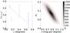 |
Fig. A.11 Left: phase curve of 26181 1996 GQ21. The continuous line indicate the best fit to Eq. (5) resulting in HV= 5.073 ± 0.050, β = (0.858 ± 0.124) mag per degree. Right: density plot showing the phase space of solutions of Eq. (5) for Δm = 0.10, in gray scale. The continuous lines show the area that contain 68.3, 95.5, and 99.7% of the solutions. |
 |
Fig. A.12 Phase curve of 1996 RQ20. The continuous line indicate the best fit to Eq. (5) resulting in HV= 7.201 ± 0.073, β = (−0.065 ± 0.075) mag per degree. |
 |
Fig. A.13 Phase curve of 1996 RR20. The continuous line indicate the best fit to Eq. (5) resulting in HV= 6.986 ± 0.128, β = (0.391 ± 0.210) mag per degree. |
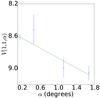 |
Fig. A.14 Phase curve of 19 299 1996 SZ4. The continuous line indicate the best fit to Eq. (5) resulting in HV= 8.564 ± 0.034, β = (0.307 ± 0.054) mag per degree. |
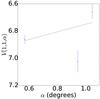 |
Fig. A.15 Phase curve of 1996 TK66. The continuous line indicate the best fit to Eq. (5) resulting in HV= 7.031 ± 0.086, β = (−0.280 ± 0.115) mag per degree. |
 |
Fig. A.16 Left: phase curve of 15 874 1996 TL66. The continuous line indicate the best fit to Eq. (5) resulting in HV= 5.257 ± 0.100, β = (0.375 ± 0.112) mag per degree. Right: density plot showing the phase space of solutions of Eq. (5) for Δm = 0.12, in gray scale. The continuous lines show the area that contain 68.3, 95.5, and 99.7% of the solutions. |
 |
Fig. A.17 Left: phase curve of 19 308 1996 TO66. The continuous line indicate the best fit to Eq. (5) resulting in HV= 4.806 ± 0.144, β = (0.150 ± 0.197) mag per degree. Right: density plot showing the phase space of solutions of Eq. (5) for Δm = 0.33, in gray scale. The continuous lines show the area that contain 68.3, 95.5, and 99.7% of the solutions. |
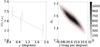 |
Fig. A.18 Left: phase curve of 15 875 1996 TP66. The continuous line indicate the best fit to Eq. (5) resulting in HV= 7.461 ± 0.084, β = (0.127 ± 0.072) mag per degree. Right: density plot showing the phase space of solutions of Eq. (5) for Δm = 0.12, in gray scale. The continuous lines show the area that contain 68.3, 95.5, and 99.7% of the solutions. |
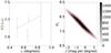 |
Fig. A.19 Left: phase curve of 118 228 1996 TQ66. The continuous line indicate the best fit to Eq. (5) resulting in HV= 8.006 ± 0.422, β = (−0.415 ± 0.680) mag per degree. Right: density plot showing the phase space of solutions of Eq. (5) for Δm = 0.22, in gray scale. The continuous lines show the area that contain 68.3, 95.5, and 99.7% of the solutions. |
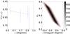 |
Fig. A.20 Left: phase curve of 1996 TS66. The continuous line indicate the best fit to Eq. (5) resulting in HV= 6.535 ± 0.167, β = (0.083 ± 0.220) mag per degree. Right: density plot showing the phase space of solutions of Eq. (5) for Δm = 0.16, in gray scale. The continuous lines show the area that contain 68.3, 95.5, and 99.7% of the solutions. |
 |
Fig. A.21 Phase curve of 33 001 1997 CU29. The continuous line indicate the best fit to Eq. (5) resulting in HV= 6.808 ± 0.057, β = (0.075 ± 0.087) mag per degree. |
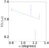 |
Fig. A.22 Phase curve of 1997 QH4. The continuous line indicate the best fit to Eq. (5) resulting in HV= 7.216 ± 0.143, β = (0.451 ± 0.142) mag per degree. |
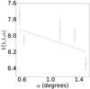 |
Fig. A.23 Phase curve of 1997 QJ4. The continuous line indicate the best fit to Eq. (5) resulting in HV= 7.754 ± 0.113, β = (0.290 ± 0.103) mag per degree. |
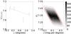 |
Fig. A.24 Left: phase curve of 91 133 1998 HK151. The continuous line indicate the best fit to Eq. (5) resulting in HV= 7.340 ± 0.056, β = (0.127 ± 0.088) mag per degree. Right: density plot showing the phase space of solutions of Eq. (5) for Δm = 0.15, in gray scale. The continuous lines show the area that contain 68.3, 95.5, and 99.7% of the solutions. |
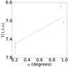 |
Fig. A.25 Phase curve of 385 194 1998 KG62. The continuous line indicate the best fit to Eq. (5) resulting in HV= 7.647 ± 0.194, β = (−0.748 ± 0.205) mag per degree. |
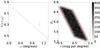 |
Fig. A.26 Left: phase curve of 26 308 1998 SM165. The continuous line indicate the best fit to Eq. (5) resulting in HV= 5.938 ± 0.363, β = (0.446 ± 0.376) mag per degree. Right: density plot showing the phase space of solutions of Eq. (5) for Δm = 0.56, in gray scale. The continuous lines show the area that contain 68.3, 95.5, and 99.7% of the solutions. |
 |
Fig. A.27 Left: phase curve of 35 671 1998 SN165. The continuous line indicate the best fit to Eq. (5) resulting in HV= 5.879 ± 0.109, β = (−0.031 ± 0.115) mag per degree. Right: density plot showing the phase space of solutions of Eq. (5) for Δm = 0.16, in gray scale. The continuous lines show the area that contain 68.3, 95.5, and 99.7% of the solutions. |
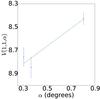 |
Fig. A.28 Phase curve of 1998 UR43. The continuous line indicate the best fit to Eq. (5) resulting in HV= 9.047 ± 0.108, β = (−0.764 ± 0.165) mag per degree. |
 |
Fig. A.29 Left: phase curve of 33 340 1998 VG44. The continuous line indicate the best fit to Eq. (5) resulting in HV= 6.599 ± 0.205, β = (0.228 ± 0.158) mag per degree. Right: density plot showing the phase space of solutions of Eq. (5) for Δm = 0.10, in gray scale. The continuous lines show the area that contain 68.3, 95.5, and 99.7% of the solutions. |
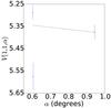 |
Fig. A.30 Phase curve of 1999 CD158. The continuous line indicate the best fit to Eq. (5) resulting in HV= 5.289 ± 0.092, β = (0.092 ± 0.119) mag per degree. |
 |
Fig. A.31 Left: phase curve of 26 375 1999 DE9. The continuous line indicate the best fit to Eq. (5) resulting in HV= 5.120 ± 0.024, β = (0.183 ± 0.032) mag per degree. Right: density plot showing the phase space of solutions of Eq. (5) for Δm = 0.10, in gray scale. The continuous lines show the area that contain 68.3, 95.5, and 99.7% of the solutions. |
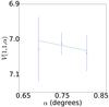 |
Fig. A.32 Phase curve of 1999 HS11. The continuous line indicate the best fit to Eq. (5) resulting in HV= 6.843 ± 0.555, β = (0.233 ± 0.728) mag per degree. |
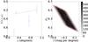 |
Fig. A.33 Left: phase curve of 40 314 1999 KR16. The continuous line indicate the best fit to Eq. (5) resulting in HV= 6.316 ± 0.139, β = (−0.126 ± 0.180) mag per degree. Right: density plot showing the phase space of solutions of Eq. (5) for Δm = 0.18, in gray scale. The continuous lines show the area that contain 68.3, 95.5, and 99.7% of the solutions. |
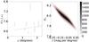 |
Fig. A.34 Left: phase curve of 44 594 1999 OX3. The continuous line indicate the best fit to Eq. (5) resulting in HV= 7.980 ± 0.092, β = (−0.086 ± 0.057) mag per degree. Right: density plot showing the phase space of solutions of Eq. (5) for Δm = 0.11, in gray scale. The continuous lines show the area that contain 68.3, 95.5, and 99.7% of the solutions. |
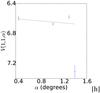 |
Fig. A.35 Phase curve of 86 047 1999 OY3. The continuous line indicate the best fit to Eq. (5) resulting in HV= 6.579 ± 0.044, β = (0.067 ± 0.042) mag per degree. |
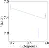 |
Fig. A.36 Phase curve of 86 177 1999 RY215. The continuous line indicate the best fit to Eq. (5) resulting in HV= 7.097 ± 0.084, β = (0.341 ± 0.111) mag per degree. |
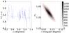 |
Fig. A.37 Left: phase curve of 47171 1999 TC36. The continuous line indicate the best fit to Eq. (5) resulting in HV= 5.395 ± 0.030, β = (0.111 ± 0.027) mag per degree. Right: density plot showing the phase space of solutions of Eq. (5) for Δm = 0.07, in gray scale. The continuous lines show the area that contain 68.3, 95.5, and 99.7% of the solutions. |
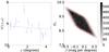 |
Fig. A.38 Left: phase curve of 29 981 1999 TD10. The continuous line indicate the best fit to Eq. (5) resulting in HV= 9.105 ± 0.430, β = (0.033 ± 0.122) mag per degree. Right: density plot showing the phase space of solutions of Eq. (5) for Δm = 0.65, in gray scale. The continuous lines show the area that contain 68.3, 95.5, and 99.7% of the solutions. |
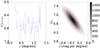 |
Fig. A.39 Left: phase curve of 47 932 2000 GN171. The continuous line indicate the best fit to Eq. (5) resulting in HV= 6.776 ± 0.243, β = (−0.101 ± 0.186) mag per degree. Right: density plot showing the phase space of solutions of Eq. (5) for Δm = 0.61, in gray scale. The continuous lines show the area that contain 68.3, 95.5, and 99.7% of the solutions. |
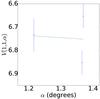 |
Fig. A.40 Phase curve of 138 537 2000 OK67. The continuous line indicate the best fit to Eq. (5) resulting in HV= 6.629 ± 0.694, β = (0.089 ± 0.518) mag per degree. |
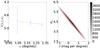 |
Fig. A.41 Left: phase curve of 82 075 2000 YW134. The continuous line indicate the best fit to Eq. (5) resulting in HV= 4.378 ± 0.687, β = (0.377 ± 0.552) mag per degree. Right: density plot showing the phase space of solutions of Eq. (5) for Δm = 0.10, in gray scale. The continuous lines show the area that contain 68.3, 95.5, and 99.7% of the solutions. |
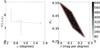 |
Fig. A.42 Left: phase curve of 82 158 2001 FP185. The continuous line indicate the best fit to Eq. (5) resulting in HV= 6.420 ± 0.062, β = (0.123 ± 0.052) mag per degree. Right: density plot showing the phase space of solutions of Eq. (5) for Δm = 0.06, in gray scale. The continuous lines show the area that contain 68.3, 95.5, and 99.7% of the solutions. |
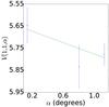 |
Fig. A.43 Phase curve of 2001 KA77. The continuous line indicate the best fit to Eq. (5) resulting in HV= 5.646 ± 0.090, β = (0.130 ± 0.095) mag per degree. |
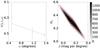 |
Fig. A.44 Left: phase curve of 2001 KD77. The continuous line indicate the best fit to Eq. (5) resulting in HV= 6.299 ± 0.099, β = (0.141 ± 0.082) mag per degree. Right: density plot showing the phase space of solutions of Eq. (5) for Δm = 0.07, in gray scale. The continuous lines show the area that contain 68.3, 95.5, and 99.7% of the solutions. |
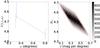 |
Fig. A.45 Left: phase curve of 42 301 2001 UR163. The continuous line indicate the best fit to Eq. (5) resulting in HV= 4.529 ± 0.063, β = (0.364 ± 0.117) mag per degree. Right: density plot showing the phase space of solutions of Eq. (5) for Δm = 0.08, in gray scale. The continuous lines show the area that contain 68.3, 95.5, and 99.7% of the solutions. |
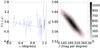 |
Fig. A.46 Left: phase curve of 55 565 2002 AW197. The continuous line indicate the best fit to Eq. (5) resulting in HV= 3.593 ± 0.023, β = (0.206 ± 0.029) mag per degree. Right: density plot showing the phase space of solutions of Eq. (5) for Δm = 0.04, in gray scale. The continuous lines show the area that contain 68.3, 95.5, and 99.7% of the solutions. |
 |
Fig. A.47 Left: phase curve of 2002 GP32. The continuous line indicate the best fit to Eq. (5) resulting in HV= 7.133 ± 0.027, β = (−0.135 ± 0.036) mag per degree. Right: density plot showing the phase space of solutions of Eq. (5) for Δm = 0.03, in gray scale. The continuous lines show the area that contain 68.3, 95.5, and 99.7% of the solutions. |
 |
Fig. A.48 Left: phase curve of 95 626 2002 GZ32. The continuous line indicate the best fit to Eq. (5) resulting in HV= 7.419 ± 0.126, β = (0.043 ± 0.064) mag per degree. Right: density plot showing the phase space of solutions of Eq. (5) for Δm = 0.15, in gray scale. The continuous lines show the area that contain 68.3, 95.5, and 99.7% of the solutions. |
 |
Fig. A.49 Phase curve of 119 951 2002 KX14. The continuous line indicate the best fit to Eq. (5) resulting in HV= 4.978 ± 0.017, β = (0.114 ± 0.031) mag per degree. |
 |
Fig. A.50 Left: phase curve of 250 112 2002 KY14. The continuous line indicate the best fit to Eq. (5) resulting in HV= 11.808 ± 0.763, β = (−0.274 ± 0.193) mag per degree. Right: density plot showing the phase space of solutions of Eq. (5) for Δm = 0.13, in gray scale. The continuous lines show the area that contain 68.3, 95.5, and 99.7% of the solutions. |
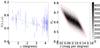 |
Fig. A.51 Left: phase curve of 73 480 2002 PN34. The continuous line indicate the best fit to Eq. (5) resulting in HV= 8.618 ± 0.054, β = (0.090 ± 0.027) mag per degree. Right: density plot showing the phase space of solutions of Eq. (5) for Δm = 0.18, in gray scale. The continuous lines show the area that contain 68.3, 95.5, and 99.7% of the solutions. |
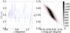 |
Fig. A.52 Left: phase curve of 55 636 2002 TX300. The continuous line indicate the best fit to Eq. (5) resulting in HV= 3.574 ± 0.055, β = (0.005 ± 0.044) mag per degree. Right: density plot showing the phase space of solutions of Eq. (5) for Δm = 0.09, in gray scale. The continuous lines show the area that contain 68.3, 95.5, and 99.7% of the solutions. |
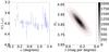 |
Fig. A.53 Left: phase curve of 55 637 2002 UX25. The continuous line indicate the best fit to Eq. (5) resulting in HV= 3.883 ± 0.048, β = (0.159 ± 0.056) mag per degree. Right: density plot showing the phase space of solutions of Eq. (5) for Δm = 0.21, in gray scale. The continuous lines show the area that contain 68.3, 95.5, and 99.7% of the solutions. |
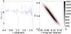 |
Fig. A.54 Left: phase curve of 55 638 2002 VE95. The continuous line indicate the best fit to Eq. (5) resulting in HV= 5.813 ± 0.037, β = (0.089 ± 0.024) mag per degree. Right: density plot showing the phase space of solutions of Eq. (5) for Δm = 0.08, in gray scale. The continuous lines show the area that contain 68.3, 95.5, and 99.7% of the solutions. |
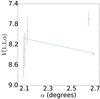 |
Fig. A.55 Phase curve of 127 546 2002 XU93. The continuous line indicate the best fit to Eq. (5) resulting in HV= 7.031 ± 0.859, β = (0.498 ± 0.320) mag per degree. |
 |
Fig. A.56 Left: phase curve of 208 996 2003 AZ84. The continuous line indicate the best fit to Eq. (5) resulting in HV= 3.779 ± 0.114, β = (0.054 ± 0.118) mag per degree. Right: density plot showing the phase space of solutions of Eq. (5) for Δm = 0.14, in gray scale. The continuous lines show the area that contain 68.3, 95.5, and 99.7% of the solutions. |
 |
Fig. A.57 Left: phase curve of 120 061 2003 CO1. The continuous line indicate the best fit to Eq. (5) resulting in HV= 9.146 ± 0.056, β = (0.092 ± 0.015) mag per degree. Right: density plot showing the phase space of solutions of Eq. (5) for Δm = 0.07, in gray scale. The continuous lines show the area that contain 68.3, 95.5, and 99.7% of the solutions. |
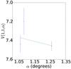 |
Fig. A.58 Phase curve of 133 067 2003 FB128. The continuous line indicate the best fit to Eq. (5) resulting in HV= 6.922 ± 0.566, β = (0.422 ± 0.469) mag per degree. |
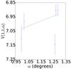 |
Fig. A.59 Phase curve of 2003 FE128. The continuous line indicate the best fit to Eq. (5) resulting in HV= 7.381 ± 0.256, β = (−0.349 ± 0.209) mag per degree. |
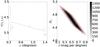 |
Fig. A.60 Left: phase curve of 120 132 2003 FY128. The continuous line indicate the best fit to Eq. (5) resulting in HV= 4.632 ± 0.187, β = (0.535 ± 0.145) mag per degree. Right: density plot showing the phase space of solutions of Eq. (5) for Δm = 0.15, in gray scale. The continuous lines show the area that contain 68.3, 95.5, and 99.7% of the solutions. |
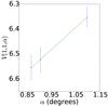 |
Fig. A.61 Phase curve of 385 437 2003 GH55. The continuous line indicate the best fit to Eq. (5) resulting in HV= 7.319 ± 0.247, β = (−0.880 ± 0.251) mag per degree. |
 |
Fig. A.62 Left: phase curve of 120 178 2003 OP32. The continuous line indicate the best fit to Eq. (5) resulting in HV= 4.067 ± 0.318, β = (0.045 ± 0.280) mag per degree. Right: density plot showing the phase space of solutions of Eq. (5) for Δm = 0.26, in gray scale. The continuous lines show the area that contain 68.3, 95.5, and 99.7% of the solutions. |
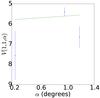 |
Fig. A.63 Phase curve of 143 707 2003 UY117. The continuous line indicate the best fit to Eq. (5) resulting in HV= 5.830 ± 1.299, β = (−0.230 ± 1.329) mag per degree. |
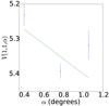 |
Fig. A.64 Phase curve of 2003 UZ117. The continuous line indicate the best fit to Eq. (5) resulting in HV= 5.185 ± 0.054, β = (0.214 ± 0.073) mag per degree. |
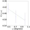 |
Fig. A.65 Phase curve of 2003 UZ413. The continuous line indicate the best fit to Eq. (5) resulting in HV= 4.361 ± 0.068, β = (0.144 ± 0.096) mag per degree. |
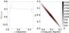 |
Fig. A.66 Left: phase curve of 136 204 2003 WL7. The continuous line indicate the best fit to Eq. (5) resulting in HV= 8.897 ± 0.149, β = (0.089 ± 0.049) mag per degree. Right: density plot showing the phase space of solutions of Eq. (5) for Δm = 0.05, in gray scale. The continuous lines show the area that contain 68.3, 95.5, and 99.7% of the solutions. |
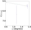 |
Fig. A.67 Phase curve of 120 216 2004 EW95. The continuous line indicate the best fit to Eq. (5) resulting in HV= 6.579 ± 0.021, β = (0.071 ± 0.024) mag per degree. |
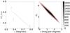 |
Fig. A.68 Left: phase curve of 90 568 2004 GV9. The continuous line indicate the best fit to Eq. (5) resulting in HV= 3.409 ± 0.357, β = (1.353 ± 0.542) mag per degree. Right: density plot showing the phase space of solutions of Eq. (5) for Δm = 0.16, in gray scale. The continuous lines show the area that contain 68.3, 95.5, and 99.7% of the solutions. |
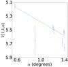 |
Fig. A.69 Phase curve of 307 982 2004 PG115. The continuous line indicate the best fit to Eq. (5) resulting in HV= 4.874 ± 0.064, β = (0.505 ± 0.051) mag per degree. |
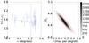 |
Fig. A.70 Left: phase curve of 120 348 2004 TY364. The continuous line indicate the best fit to Eq. (5) resulting in HV= 4.519 ± 0.137, β = (0.146 ± 0.103) mag per degree. Right: density plot showing the phase space of solutions of Eq. (5) for Δm = 0.22, in gray scale. The continuous lines show the area that contain 68.3, 95.5, and 99.7% of the solutions. |
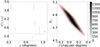 |
Fig. A.71 Left: phase curve of 144 897 2004 UX10. The continuous line indicate the best fit to Eq. (5) resulting in HV= 4.825 ± 0.097, β = (0.061 ± 0.103) mag per degree. Right: density plot showing the phase space of solutions of Eq. (5) for Δm = 0.08, in gray scale. The continuous lines show the area that contain 68.3, 95.5, and 99.7% of the solutions. |
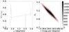 |
Fig. A.72 Left: phase curve of 230 965 2004 XA192. The continuous line indicate the best fit to Eq. (5) resulting in HV= 5.059 ± 0.085, β = (−0.175 ± 0.070) mag per degree. Right: density plot showing the phase space of solutions of Eq. (5) for Δm = 0.07, in gray scale. The continuous lines show the area that contain 68.3, 95.5, and 99.7% of the solutions. |
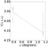 |
Fig. A.73 Phase curve of 303 775 2005 QU182. The continuous line indicate the best fit to Eq. (5) resulting in HV= 3.853 ± 0.028, β = (0.277 ± 0.034) mag per degree. |
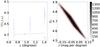 |
Fig. A.74 Left: phase curve of 145 451 2005 RM43. The continuous line indicate the best fit to Eq. (5) resulting in HV= 4.704 ± 0.081, β = (−0.028 ± 0.064) mag per degree. Right: density plot showing the phase space of solutions of Eq. (5) for Δm = 0.04, in gray scale. The continuous lines show the area that contain 68.3, 95.5, and 99.7% of the solutions. |
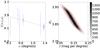 |
Fig. A.75 Left: phase curve of 145 452 2005 RN43. The continuous line indicate the best fit to Eq. (5) resulting in HV= 3.882 ± 0.036, β = (0.138 ± 0.030) mag per degree. Right: density plot showing the phase space of solutions of Eq. (5) for Δm = 0.04, in gray scale. The continuous lines show the area that contain 68.3, 95.5, and 99.7% of the solutions. |
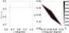 |
Fig. A.76 Left: phase curve of 145 453 2005 RR43. The continuous line indicate the best fit to Eq. (5) resulting in HV= 4.252 ± 0.067, β = (−0.003 ± 0.065) mag per degree. Right: density plot showing the phase space of solutions of Eq. (5) for Δm = 0.06, in gray scale. The continuous lines show the area that contain 68.3, 95.5, and 99.7% of the solutions. |
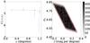 |
Fig. A.77 Left: phase curve of 145 480 2005 TB190. The continuous line indicate the best fit to Eq. (5) resulting in HV= 4.676 ± 0.084, β = (0.052 ± 0.106) mag per degree. Right: density plot showing the phase space of solutions of Eq. (5) for Δm = 0.12, in gray scale. The continuous lines show the area that contain 68.3, 95.5, and 99.7% of the solutions. |
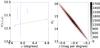 |
Fig. A.78 Left: phase curve of 145 486 2005 UJ438. The continuous line indicate the best fit to Eq. (5) resulting in HV= 14.602 ± 0.617, β = (−0.412 ± 0.098) mag per degree. Right: density plot showing the phase space of solutions of Eq. (5) for Δm = 0.13, in gray scale. The continuous lines show the area that contain 68.3, 95.5, and 99.7% of the solutions. |
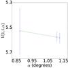 |
Fig. A.79 Phase curve of 2007 OC10. The continuous line indicate the best fit to Eq. (5) resulting in HV= 5.330 ± 0.825, β = (0.223 ± 0.740) mag per degree. |
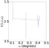 |
Fig. A.80 Phase curve of 225 088 2007 OR10. The continuous line indicate the best fit to Eq. (5) resulting in HV= 2.316 ± 0.124, β = (0.257 ± 0.505) mag per degree. |
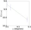 |
Fig. A.81 Phase curve of 281 371 2008 FC76. The continuous line indicate the best fit to Eq. (5) resulting in HV= 9.488 ± 0.074, β = (0.101 ± 0.015) mag per degree. |
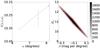 |
Fig. A.82 Left: phase curve of 342 842 2008 YB3. The continuous line indicate the best fit to Eq. (5) resulting in HV= 11.024 ± 0.696, β = (−0.104 ± 0.095) mag per degree. Right: density plot showing the phase space of solutions of Eq. (5) for Δm = 0.20, in gray scale. The continuous lines show the area that contain 68.3, 95.5, and 99.7% of the solutions. |
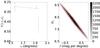 |
Fig. A.83 Left: phase curve of 55 576 Amycus. The continuous line indicate the best fit to Eq. (5) resulting in HV= 8.213 ± 0.621, β = (0.052 ± 0.351) mag per degree. Right: density plot showing the phase space of solutions of Eq. (5) for Δm = 0.16, in gray scale. The continuous lines show the area that contain 68.3, 95.5, and 99.7% of the solutions. |
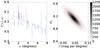 |
Fig. A.84 Left: phase curve of 8405 Asbolus. The continuous line indicate the best fit to Eq. (5) resulting in HV= 9.138 ± 0.130, β = (0.042 ± 0.029) mag per degree. Right: density plot showing the phase space of solutions of Eq. (5) for Δm = 0.55, in gray scale. The continuous lines show the area that contain 68.3, 95.5, and 99.7% of the solutions. |
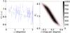 |
Fig. A.85 Left: phase curve of 54 598 Bienor. The continuous line indicate the best fit to Eq. (5) resulting in HV= 7.656 ± 0.443, β = (0.130 ± 0.170) mag per degree. Right: density plot showing the phase space of solutions of Eq. (5) for Δm = 0.75, in gray scale. The continuous lines show the area that contain 68.3, 95.5, and 99.7% of the solutions. |
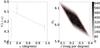 |
Fig. A.86 Left: phase curve of 66 652 Borasisi. The continuous line indicate the best fit to Eq. (5) resulting in HV= 6.032 ± 0.040, β = (0.231 ± 0.062) mag per degree. Right: density plot showing the phase space of solutions of Eq. (5) for Δm = 0.05, in gray scale. The continuous lines show the area that contain 68.3, 95.5, and 99.7% of the solutions. |
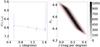 |
Fig. A.87 Left: phase curve of 65 489 Ceto. The continuous line indicate the best fit to Eq. (5) resulting in HV= 6.573 ± 0.126, β = (0.196 ± 0.096) mag per degree. Right: density plot showing the phase space of solutions of Eq. (5) for Δm = 0.13, in gray scale. The continuous lines show the area that contain 68.3, 95.5, and 99.7% of the solutions. |
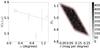 |
Fig. A.88 Left: phase curve of 19521 Chaos. The continuous line indicate the best fit to Eq. (5) resulting in HV= 4.987 ± 0.065, β = (0.102 ± 0.070) mag per degree. Right: density plot showing the phase space of solutions of Eq. (5) for Δm = 0.10, in gray scale. The continuous lines show the area that contain 68.3, 95.5, and 99.7% of the solutions. |
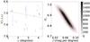 |
Fig. A.89 Left: phase curve of 10 199 Chariklo. The continuous line indicate the best fit to Eq. (5) resulting in HV= 6.870 ± 0.055, β = (0.064 ± 0.016) mag per degree. Right: density plot showing the phase space of solutions of Eq. (5) for Δm = 0.10, in gray scale. The continuous lines show the area that contain 68.3, 95.5, and 99.7% of the solutions. |
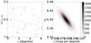 |
Fig. A.90 Left: phase curve of 2060 Chiron. The continuous line indicate the best fit to Eq. (5) resulting in HV= 6.399 ± 0.019, β = (0.083 ± 0.005) mag per degree. Right: density plot showing the phase space of solutions of Eq. (5) for Δm = 0.09, in gray scale. The continuous lines show the area that contain 68.3, 95.5, and 99.7% of the solutions. |
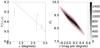 |
Fig. A.91 Left: phase curve of 83982 Crantor. The continuous line indicate the best fit to Eq. (5) resulting in HV= 9.096 ± 0.405, β = (0.110 ± 0.149) mag per degree. Right: density plot showing the phase space of solutions of Eq. (5) for Δm = 0.34, in gray scale. The continuous lines show the area that contain 68.3, 95.5, and 99.7% of the solutions. |
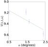 |
Fig. A.92 Phase curve of 52 975 Cyllarus. The continuous line indicate the best fit to Eq. (5) resulting in HV= 9.064 ± 0.041, β = (0.184 ± 0.029) mag per degree. |
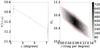 |
Fig. A.93 Left: phase curve of 31 824 Elatus. The continuous line indicate the best fit to Eq. (5) resulting in HV= 10.592 ± 0.171, β = (0.078 ± 0.031) mag per degree. Right: density plot showing the phase space of solutions of Eq. (5) for Δm = 0.24, in gray scale. The continuous lines show the area that contain 68.3, 95.5, and 99.7% of the solutions. |
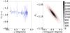 |
Fig. A.94 Left: phase curve of 136 199 Eris. The continuous line indicate the best fit to Eq. (5) resulting in HV=−1.124 ± 0.025, β = (0.119 ± 0.056) mag per degree. Right: density plot showing the phase space of solutions of Eq. (5) for Δm = 0.10, in gray scale. The continuous lines show the area that contain 68.3, 95.5, and 99.7% of the solutions. |
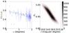 |
Fig. A.95 Left: phase curve of 38 628 Huya. The continuous line indicate the best fit to Eq. (5) resulting in HV= 4.975 ± 0.037, β = (0.173 ± 0.026) mag per degree. Right: density plot showing the phase space of solutions of Eq. (5) for Δm = 0.10, in gray scale. The continuous lines show the area that contain 68.3, 95.5, and 99.7% of the solutions. |
 |
Fig. A.96 Left: phase curve of 28978 Ixion. The continuous line indicate the best fit to Eq. (5) resulting in HV= 3.774 ± 0.021, β = (0.194 ± 0.031) mag per degree. Right: density plot showing the phase space of solutions of Eq. (5) for Δm = 0.05, in gray scale. The continuous lines show the area that contain 68.3, 95.5, and 99.7% of the solutions. |
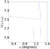 |
Fig. A.97 Phase curve of 58534 Logos. The continuous line indicate the best fit to Eq. (5) resulting in HV= 7.411 ± 0.041, β = (0.055 ± 0.057) mag per degree. |
 |
Fig. A.98 Left: phase curve of 136472 Makemake. The continuous line indicate the best fit to Eq. (5) resulting in HV= 0.009 ± 0.012, β = (0.202 ± 0.015) mag per degree. Right: density plot showing the phase space of solutions of Eq. (5) for Δm = 0.03, in gray scale. The continuous lines show the area that contain 68.3, 95.5, and 99.7% of the solutions. |
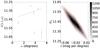 |
Fig. A.99 Left: phase curve of 52 872 Okyrhoe. The continuous line indicate the best fit to Eq. (5) resulting in HV= 11.441 ± 0.062, β = (−0.023 ± 0.017) mag per degree. Right: density plot showing the phase space of solutions of Eq. (5) for Δm = 0.07, in gray scale. The continuous lines show the area that contain 68.3, 95.5, and 99.7% of the solutions. |
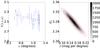 |
Fig. A.100 Left: phase curve of 90 482 Orcus. The continuous line indicate the best fit to Eq. (5) resulting in HV= 2.280 ± 0.021, β = (0.160 ± 0.022) mag per degree. Right: density plot showing the phase space of solutions of Eq. (5) for Δm = 0.04, in gray scale. The continuous lines show the area that contain 68.3, 95.5, and 99.7% of the solutions. |
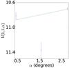 |
Fig. A.101 Phase curve of 49 036 Pelion. The continuous line indicate the best fit to Eq. (5) resulting in HV= 10.911 ± 0.069, β = (−0.074 ± 0.026) mag per degree. |
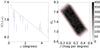 |
Fig. A.102 Left: phase curve of 5145 Pholus. The continuous line indicate the best fit to Eq. (5) resulting in HV= 7.474 ± 0.309, β = (0.153 ± 0.156) mag per degree. Right: density plot showing the phase space of solutions of Eq. (5) for Δm = 0.60, in gray scale. The continuous lines show the area that contain 68.3, 95.5, and 99.7% of the solutions. |
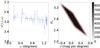 |
Fig. A.103 Left: phase curve of 50 000 Quaoar. The continuous line indicate the best fit to Eq. (5) resulting in HV= 2.777 ± 0.250, β = (0.117 ± 0.221) mag per degree. Right: density plot showing the phase space of solutions of Eq. (5) for Δm = 0.30, in gray scale. The continuous lines show the area that contain 68.3, 95.5, and 99.7% of the solutions. |
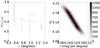 |
Fig. A.104 Left: phase curve of 120347 Salacia. The continuous line indicate the best fit to Eq. (5) resulting in HV= 4.151 ± 0.030, β = (0.132 ± 0.028) mag per degree. Right: density plot showing the phase space of solutions of Eq. (5) for Δm = 0.03, in gray scale. The continuous lines show the area that contain 68.3, 95.5, and 99.7% of the solutions. |
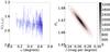 |
Fig. A.105 Left: phase curve of 90377 Sedna. The continuous line indicate the best fit to Eq. (5) resulting in HV= 1.669 ± 0.004, β = (0.266 ± 0.008) mag per degree. Right: density plot showing the phase space of solutions of Eq. (5) for Δm = 0.02, in gray scale. The continuous lines show the area that contain 68.3, 95.5, and 99.7% of the solutions. |
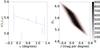 |
Fig. A.106 Left: phase curve of 79360 Sila-Numan. The continuous line indicate the best fit to Eq. (5) resulting in HV= 5.573 ± 0.224, β = (0.095 ± 0.209) mag per degree. Right: density plot showing the phase space of solutions of Eq. (5) for Δm = 0.22, in gray scale. The continuous lines show the area that contain 68.3, 95.5, and 99.7% of the solutions. |
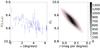 |
Fig. A.107 Left: phase curve of 32532 Thereus. The continuous line indicate the best fit to Eq. (5) resulting in HV= 9.454 ± 0.137, β = (0.061 ± 0.034) mag per degree. Right: density plot showing the phase space of solutions of Eq. (5) for Δm = 0.34, in gray scale. The continuous lines show the area that contain 68.3, 95.5, and 99.7% of the solutions. |
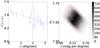 |
Fig. A.108 Left: phase curve of 42355 Typhon. The continuous line indicate the best fit to Eq. (5) resulting in HV= 7.670 ± 0.026, β = (0.128 ± 0.013) mag per degree. Right: density plot showing the phase space of solutions of Eq. (5) for Δm = 0.07, in gray scale. The continuous lines show the area that contain 68.3, 95.5, and 99.7% of the solutions. |
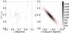 |
Fig. A.109 Left: phase curve of 174567 Varda. The continuous line indicate the best fit to Eq. (5) resulting in HV= 3.988 ± 0.048, β = (−0.455 ± 0.071) mag per degree. Right: density plot showing the phase space of solutions of Eq. (5) for Δm = 0.06, in gray scale. The continuous lines show the area that contain 68.3, 95.5, and 99.7% of the solutions. |
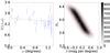 |
Fig. A.110 Left: phase curve of 20 000 Varuna. The continuous line indicate the best fit to Eq. (5) resulting in HV= 3.966 ± 0.233, β = (0.104 ± 0.246) mag per degree. Right: density plot showing the phase space of solutions of Eq. (5) for Δm = 0.50, in gray scale. The continuous lines show the area that contain 68.3, 95.5, and 99.7% of the solutions. |
All Tables
Comparison between the values of HV and β from this work with those from three selected references.
All Figures
|
Fig. 1 Color−magnitude diagram for the objects in our database. We show in red the objects that have at least one color measured by us, while objects whose data come from the literature alone are shown in blue. The (V−R)⊙ is shown for reference as a horizontal line. |
| In the text | |
|
Fig. 2 Example of phase curve of 1996 TL66. Left: scatter plot of V(1,1,α) versus α. The line represents the solution for HV and β as mentioned in the text. Right: density plot showing the phase space of solutions of Eq. (5) when Δm ≠ 0, in gray scale. The effect of the Δm may cause values between 5.0 and 5.5 for HV, while the same is true for β ∈ (0.041,0.706) mag per degree. The continuous lines (red) show the area that contains 68.3, 95.5, and 99.7% of the solutions. |
| In the text | |
|
Fig. 3 Histogram showing the HV distribution. |
| In the text | |
|
Fig. 4 Histogram showing the β distribution. The dashed black line is the better fit to the distribution, modeled as the sum of two Gaussian distributions (see text). Each individual Gaussian distribution is shown as continuous green and dotted red lines. |
| In the text | |
|
Fig. 5 Left: scatter plot of HV vs. semi-major axis. Right: outcome of the 10 000 realizations in form of a two-dimensional histogram in rs and Prs which shows the phase space where the solutions lie. In a few cases it is relatively clear that a correlation might exists, while in some other cases large excursions are seen, which indicate that a false correlation could arise in the case of large errors. |
| In the text | |
|
Fig. 6 Left: scatter plot of HV as measured by us vs. (ours). HV as used within the “TNO’s are cool” program (HSO). Right: two-dimensional histogram showing the most likely correlations. |
| In the text | |
|
Fig. 7 Left: scatter plot of HV vs. the geometric albedo measured by the “TNOs are cool” program. Right: two-dimensional histogram showing the most likely correlations. |
| In the text | |
|
Fig. 8 Left: scatter plot of β vs. HV. Right: two-dimensional histogram showing the most likely correlations. |
| In the text | |
|
Fig. 9 Left: scatter plot of HV vs. Δm. Right: Two-dimensional histogram showing the most likely correlations. |
| In the text | |
|
Fig. 10 Left: scatter plot of HV vs. eccentricity. Right: two-dimensional histogram showing the most likely correlations. |
| In the text | |
|
Fig. 11 Left: scatter plot of HV vs. inclination. Right: two-dimensional histogram showing the most likely correlations. |
| In the text | |
|
Fig. A.1 Phase curve of 15 760 1992 QB1. The continuous line indicate the best fit to Eq. (5) resulting in HV= 7.839 ± 0.097, β = (−0.193 ± 0.132) mag per degree. |
| In the text | |
|
Fig. A.2 Phase curve of 15 788 1993 SB. The continuous line indicate the best fit to Eq. (5) resulting in HV= 7.995 ± 0.059, β = (0.374 ± 0.066) mag per degree. |
| In the text | |
|
Fig. A.3 Left: phase curve of 15 789 1993 SC. The continuous line indicate the best fit to Eq. (5) resulting in HV= 7.393 ± 0.020, β = (0.050 ± 0.017) mag per degree. Right: density plot showing the phase space of solutions of Eq. (5) for Δm = 0.04, in gray scale. The continuous lines show the area that contain 68.3, 95.5, and 99.7% of the solutions. |
| In the text | |
|
Fig. A.4 Phase curve of 1994 EV3. The continuous line indicate the best fit to Eq. (5) resulting in HV= 8.183 ± 0.247, β = (−0.803 ± 0.329) mag per degree. |
| In the text | |
|
Fig. A.5 Phase curve of 16 684 1994 JQ1. The continuous line indicate the best fit to Eq. (5) resulting in HV= 7.031 ± 0.078, β = (0.570 ± 0.125) mag per degree. |
| In the text | |
|
Fig. A.6 Left: phase curve of 15 820 1994 TB. The continuous line indicate the best fit to Eq. (5) resulting in HV= 8.017 ± 0.226, β = (0.133 ± 0.152) mag per degree. Right: density plot showing the phase space of solutions of Eq. (5) for Δm = 0.34, in gray scale. The continuous lines show the area that contain 68.3, 95.5, and 99.7% of the solutions. |
| In the text | |
|
Fig. A.7 Left: phase curve of 19 255 1994 VK8. The continuous line indicate the best fit to Eq. (5) resulting in HV= 7.840 ± 0.923, β = (−0.173 ± 0.976) mag per degree. Right: density plot showing the phase space of solutions of Eq. (5) for Δm = 0.42, in gray scale. The continuous lines show the area that contain 68.3, 95.5, and 99.7% of the solutions. |
| In the text | |
|
Fig. A.8 Phase curve of 1995 HM5. The continuous line indicate the best fit to Eq. (5) resulting in HV= 8.315 ± 0.100, β = (0.037 ± 0.074) mag per degree. |
| In the text | |
|
Fig. A.9 Left: phase curve of 32 929 1995 QY9. The continuous line indicate the best fit to Eq. (5) resulting in HV= 8.136 ± 0.515, β = (−0.108 ± 0.459) mag per degree. Right: density plot showing the phase space of solutions of Eq. (5) for Δm = 0.60, in gray scale. The continuous lines show the area that contain 68.3, 95.5, and 99.7% of the solutions. |
| In the text | |
|
Fig. A.10 Left: phase curve of 24 835 1995 SM55. The continuous line indicate the best fit to Eq. (5) resulting in HV= 4.584 ± 0.178, β = (0.139 ± 0.198) mag per degree. Right: density plot showing the phase space of solutions of Eq. (5) for Δm = 0.19, in gray scale. The continuous lines show the area that contain 68.3, 95.5, and 99.7% of the solutions. |
| In the text | |
|
Fig. A.11 Left: phase curve of 26181 1996 GQ21. The continuous line indicate the best fit to Eq. (5) resulting in HV= 5.073 ± 0.050, β = (0.858 ± 0.124) mag per degree. Right: density plot showing the phase space of solutions of Eq. (5) for Δm = 0.10, in gray scale. The continuous lines show the area that contain 68.3, 95.5, and 99.7% of the solutions. |
| In the text | |
|
Fig. A.12 Phase curve of 1996 RQ20. The continuous line indicate the best fit to Eq. (5) resulting in HV= 7.201 ± 0.073, β = (−0.065 ± 0.075) mag per degree. |
| In the text | |
|
Fig. A.13 Phase curve of 1996 RR20. The continuous line indicate the best fit to Eq. (5) resulting in HV= 6.986 ± 0.128, β = (0.391 ± 0.210) mag per degree. |
| In the text | |
|
Fig. A.14 Phase curve of 19 299 1996 SZ4. The continuous line indicate the best fit to Eq. (5) resulting in HV= 8.564 ± 0.034, β = (0.307 ± 0.054) mag per degree. |
| In the text | |
|
Fig. A.15 Phase curve of 1996 TK66. The continuous line indicate the best fit to Eq. (5) resulting in HV= 7.031 ± 0.086, β = (−0.280 ± 0.115) mag per degree. |
| In the text | |
|
Fig. A.16 Left: phase curve of 15 874 1996 TL66. The continuous line indicate the best fit to Eq. (5) resulting in HV= 5.257 ± 0.100, β = (0.375 ± 0.112) mag per degree. Right: density plot showing the phase space of solutions of Eq. (5) for Δm = 0.12, in gray scale. The continuous lines show the area that contain 68.3, 95.5, and 99.7% of the solutions. |
| In the text | |
|
Fig. A.17 Left: phase curve of 19 308 1996 TO66. The continuous line indicate the best fit to Eq. (5) resulting in HV= 4.806 ± 0.144, β = (0.150 ± 0.197) mag per degree. Right: density plot showing the phase space of solutions of Eq. (5) for Δm = 0.33, in gray scale. The continuous lines show the area that contain 68.3, 95.5, and 99.7% of the solutions. |
| In the text | |
|
Fig. A.18 Left: phase curve of 15 875 1996 TP66. The continuous line indicate the best fit to Eq. (5) resulting in HV= 7.461 ± 0.084, β = (0.127 ± 0.072) mag per degree. Right: density plot showing the phase space of solutions of Eq. (5) for Δm = 0.12, in gray scale. The continuous lines show the area that contain 68.3, 95.5, and 99.7% of the solutions. |
| In the text | |
|
Fig. A.19 Left: phase curve of 118 228 1996 TQ66. The continuous line indicate the best fit to Eq. (5) resulting in HV= 8.006 ± 0.422, β = (−0.415 ± 0.680) mag per degree. Right: density plot showing the phase space of solutions of Eq. (5) for Δm = 0.22, in gray scale. The continuous lines show the area that contain 68.3, 95.5, and 99.7% of the solutions. |
| In the text | |
|
Fig. A.20 Left: phase curve of 1996 TS66. The continuous line indicate the best fit to Eq. (5) resulting in HV= 6.535 ± 0.167, β = (0.083 ± 0.220) mag per degree. Right: density plot showing the phase space of solutions of Eq. (5) for Δm = 0.16, in gray scale. The continuous lines show the area that contain 68.3, 95.5, and 99.7% of the solutions. |
| In the text | |
|
Fig. A.21 Phase curve of 33 001 1997 CU29. The continuous line indicate the best fit to Eq. (5) resulting in HV= 6.808 ± 0.057, β = (0.075 ± 0.087) mag per degree. |
| In the text | |
|
Fig. A.22 Phase curve of 1997 QH4. The continuous line indicate the best fit to Eq. (5) resulting in HV= 7.216 ± 0.143, β = (0.451 ± 0.142) mag per degree. |
| In the text | |
|
Fig. A.23 Phase curve of 1997 QJ4. The continuous line indicate the best fit to Eq. (5) resulting in HV= 7.754 ± 0.113, β = (0.290 ± 0.103) mag per degree. |
| In the text | |
|
Fig. A.24 Left: phase curve of 91 133 1998 HK151. The continuous line indicate the best fit to Eq. (5) resulting in HV= 7.340 ± 0.056, β = (0.127 ± 0.088) mag per degree. Right: density plot showing the phase space of solutions of Eq. (5) for Δm = 0.15, in gray scale. The continuous lines show the area that contain 68.3, 95.5, and 99.7% of the solutions. |
| In the text | |
|
Fig. A.25 Phase curve of 385 194 1998 KG62. The continuous line indicate the best fit to Eq. (5) resulting in HV= 7.647 ± 0.194, β = (−0.748 ± 0.205) mag per degree. |
| In the text | |
|
Fig. A.26 Left: phase curve of 26 308 1998 SM165. The continuous line indicate the best fit to Eq. (5) resulting in HV= 5.938 ± 0.363, β = (0.446 ± 0.376) mag per degree. Right: density plot showing the phase space of solutions of Eq. (5) for Δm = 0.56, in gray scale. The continuous lines show the area that contain 68.3, 95.5, and 99.7% of the solutions. |
| In the text | |
|
Fig. A.27 Left: phase curve of 35 671 1998 SN165. The continuous line indicate the best fit to Eq. (5) resulting in HV= 5.879 ± 0.109, β = (−0.031 ± 0.115) mag per degree. Right: density plot showing the phase space of solutions of Eq. (5) for Δm = 0.16, in gray scale. The continuous lines show the area that contain 68.3, 95.5, and 99.7% of the solutions. |
| In the text | |
|
Fig. A.28 Phase curve of 1998 UR43. The continuous line indicate the best fit to Eq. (5) resulting in HV= 9.047 ± 0.108, β = (−0.764 ± 0.165) mag per degree. |
| In the text | |
|
Fig. A.29 Left: phase curve of 33 340 1998 VG44. The continuous line indicate the best fit to Eq. (5) resulting in HV= 6.599 ± 0.205, β = (0.228 ± 0.158) mag per degree. Right: density plot showing the phase space of solutions of Eq. (5) for Δm = 0.10, in gray scale. The continuous lines show the area that contain 68.3, 95.5, and 99.7% of the solutions. |
| In the text | |
|
Fig. A.30 Phase curve of 1999 CD158. The continuous line indicate the best fit to Eq. (5) resulting in HV= 5.289 ± 0.092, β = (0.092 ± 0.119) mag per degree. |
| In the text | |
|
Fig. A.31 Left: phase curve of 26 375 1999 DE9. The continuous line indicate the best fit to Eq. (5) resulting in HV= 5.120 ± 0.024, β = (0.183 ± 0.032) mag per degree. Right: density plot showing the phase space of solutions of Eq. (5) for Δm = 0.10, in gray scale. The continuous lines show the area that contain 68.3, 95.5, and 99.7% of the solutions. |
| In the text | |
|
Fig. A.32 Phase curve of 1999 HS11. The continuous line indicate the best fit to Eq. (5) resulting in HV= 6.843 ± 0.555, β = (0.233 ± 0.728) mag per degree. |
| In the text | |
|
Fig. A.33 Left: phase curve of 40 314 1999 KR16. The continuous line indicate the best fit to Eq. (5) resulting in HV= 6.316 ± 0.139, β = (−0.126 ± 0.180) mag per degree. Right: density plot showing the phase space of solutions of Eq. (5) for Δm = 0.18, in gray scale. The continuous lines show the area that contain 68.3, 95.5, and 99.7% of the solutions. |
| In the text | |
|
Fig. A.34 Left: phase curve of 44 594 1999 OX3. The continuous line indicate the best fit to Eq. (5) resulting in HV= 7.980 ± 0.092, β = (−0.086 ± 0.057) mag per degree. Right: density plot showing the phase space of solutions of Eq. (5) for Δm = 0.11, in gray scale. The continuous lines show the area that contain 68.3, 95.5, and 99.7% of the solutions. |
| In the text | |
|
Fig. A.35 Phase curve of 86 047 1999 OY3. The continuous line indicate the best fit to Eq. (5) resulting in HV= 6.579 ± 0.044, β = (0.067 ± 0.042) mag per degree. |
| In the text | |
|
Fig. A.36 Phase curve of 86 177 1999 RY215. The continuous line indicate the best fit to Eq. (5) resulting in HV= 7.097 ± 0.084, β = (0.341 ± 0.111) mag per degree. |
| In the text | |
|
Fig. A.37 Left: phase curve of 47171 1999 TC36. The continuous line indicate the best fit to Eq. (5) resulting in HV= 5.395 ± 0.030, β = (0.111 ± 0.027) mag per degree. Right: density plot showing the phase space of solutions of Eq. (5) for Δm = 0.07, in gray scale. The continuous lines show the area that contain 68.3, 95.5, and 99.7% of the solutions. |
| In the text | |
|
Fig. A.38 Left: phase curve of 29 981 1999 TD10. The continuous line indicate the best fit to Eq. (5) resulting in HV= 9.105 ± 0.430, β = (0.033 ± 0.122) mag per degree. Right: density plot showing the phase space of solutions of Eq. (5) for Δm = 0.65, in gray scale. The continuous lines show the area that contain 68.3, 95.5, and 99.7% of the solutions. |
| In the text | |
|
Fig. A.39 Left: phase curve of 47 932 2000 GN171. The continuous line indicate the best fit to Eq. (5) resulting in HV= 6.776 ± 0.243, β = (−0.101 ± 0.186) mag per degree. Right: density plot showing the phase space of solutions of Eq. (5) for Δm = 0.61, in gray scale. The continuous lines show the area that contain 68.3, 95.5, and 99.7% of the solutions. |
| In the text | |
|
Fig. A.40 Phase curve of 138 537 2000 OK67. The continuous line indicate the best fit to Eq. (5) resulting in HV= 6.629 ± 0.694, β = (0.089 ± 0.518) mag per degree. |
| In the text | |
|
Fig. A.41 Left: phase curve of 82 075 2000 YW134. The continuous line indicate the best fit to Eq. (5) resulting in HV= 4.378 ± 0.687, β = (0.377 ± 0.552) mag per degree. Right: density plot showing the phase space of solutions of Eq. (5) for Δm = 0.10, in gray scale. The continuous lines show the area that contain 68.3, 95.5, and 99.7% of the solutions. |
| In the text | |
|
Fig. A.42 Left: phase curve of 82 158 2001 FP185. The continuous line indicate the best fit to Eq. (5) resulting in HV= 6.420 ± 0.062, β = (0.123 ± 0.052) mag per degree. Right: density plot showing the phase space of solutions of Eq. (5) for Δm = 0.06, in gray scale. The continuous lines show the area that contain 68.3, 95.5, and 99.7% of the solutions. |
| In the text | |
|
Fig. A.43 Phase curve of 2001 KA77. The continuous line indicate the best fit to Eq. (5) resulting in HV= 5.646 ± 0.090, β = (0.130 ± 0.095) mag per degree. |
| In the text | |
|
Fig. A.44 Left: phase curve of 2001 KD77. The continuous line indicate the best fit to Eq. (5) resulting in HV= 6.299 ± 0.099, β = (0.141 ± 0.082) mag per degree. Right: density plot showing the phase space of solutions of Eq. (5) for Δm = 0.07, in gray scale. The continuous lines show the area that contain 68.3, 95.5, and 99.7% of the solutions. |
| In the text | |
|
Fig. A.45 Left: phase curve of 42 301 2001 UR163. The continuous line indicate the best fit to Eq. (5) resulting in HV= 4.529 ± 0.063, β = (0.364 ± 0.117) mag per degree. Right: density plot showing the phase space of solutions of Eq. (5) for Δm = 0.08, in gray scale. The continuous lines show the area that contain 68.3, 95.5, and 99.7% of the solutions. |
| In the text | |
|
Fig. A.46 Left: phase curve of 55 565 2002 AW197. The continuous line indicate the best fit to Eq. (5) resulting in HV= 3.593 ± 0.023, β = (0.206 ± 0.029) mag per degree. Right: density plot showing the phase space of solutions of Eq. (5) for Δm = 0.04, in gray scale. The continuous lines show the area that contain 68.3, 95.5, and 99.7% of the solutions. |
| In the text | |
|
Fig. A.47 Left: phase curve of 2002 GP32. The continuous line indicate the best fit to Eq. (5) resulting in HV= 7.133 ± 0.027, β = (−0.135 ± 0.036) mag per degree. Right: density plot showing the phase space of solutions of Eq. (5) for Δm = 0.03, in gray scale. The continuous lines show the area that contain 68.3, 95.5, and 99.7% of the solutions. |
| In the text | |
|
Fig. A.48 Left: phase curve of 95 626 2002 GZ32. The continuous line indicate the best fit to Eq. (5) resulting in HV= 7.419 ± 0.126, β = (0.043 ± 0.064) mag per degree. Right: density plot showing the phase space of solutions of Eq. (5) for Δm = 0.15, in gray scale. The continuous lines show the area that contain 68.3, 95.5, and 99.7% of the solutions. |
| In the text | |
|
Fig. A.49 Phase curve of 119 951 2002 KX14. The continuous line indicate the best fit to Eq. (5) resulting in HV= 4.978 ± 0.017, β = (0.114 ± 0.031) mag per degree. |
| In the text | |
|
Fig. A.50 Left: phase curve of 250 112 2002 KY14. The continuous line indicate the best fit to Eq. (5) resulting in HV= 11.808 ± 0.763, β = (−0.274 ± 0.193) mag per degree. Right: density plot showing the phase space of solutions of Eq. (5) for Δm = 0.13, in gray scale. The continuous lines show the area that contain 68.3, 95.5, and 99.7% of the solutions. |
| In the text | |
|
Fig. A.51 Left: phase curve of 73 480 2002 PN34. The continuous line indicate the best fit to Eq. (5) resulting in HV= 8.618 ± 0.054, β = (0.090 ± 0.027) mag per degree. Right: density plot showing the phase space of solutions of Eq. (5) for Δm = 0.18, in gray scale. The continuous lines show the area that contain 68.3, 95.5, and 99.7% of the solutions. |
| In the text | |
|
Fig. A.52 Left: phase curve of 55 636 2002 TX300. The continuous line indicate the best fit to Eq. (5) resulting in HV= 3.574 ± 0.055, β = (0.005 ± 0.044) mag per degree. Right: density plot showing the phase space of solutions of Eq. (5) for Δm = 0.09, in gray scale. The continuous lines show the area that contain 68.3, 95.5, and 99.7% of the solutions. |
| In the text | |
|
Fig. A.53 Left: phase curve of 55 637 2002 UX25. The continuous line indicate the best fit to Eq. (5) resulting in HV= 3.883 ± 0.048, β = (0.159 ± 0.056) mag per degree. Right: density plot showing the phase space of solutions of Eq. (5) for Δm = 0.21, in gray scale. The continuous lines show the area that contain 68.3, 95.5, and 99.7% of the solutions. |
| In the text | |
|
Fig. A.54 Left: phase curve of 55 638 2002 VE95. The continuous line indicate the best fit to Eq. (5) resulting in HV= 5.813 ± 0.037, β = (0.089 ± 0.024) mag per degree. Right: density plot showing the phase space of solutions of Eq. (5) for Δm = 0.08, in gray scale. The continuous lines show the area that contain 68.3, 95.5, and 99.7% of the solutions. |
| In the text | |
|
Fig. A.55 Phase curve of 127 546 2002 XU93. The continuous line indicate the best fit to Eq. (5) resulting in HV= 7.031 ± 0.859, β = (0.498 ± 0.320) mag per degree. |
| In the text | |
|
Fig. A.56 Left: phase curve of 208 996 2003 AZ84. The continuous line indicate the best fit to Eq. (5) resulting in HV= 3.779 ± 0.114, β = (0.054 ± 0.118) mag per degree. Right: density plot showing the phase space of solutions of Eq. (5) for Δm = 0.14, in gray scale. The continuous lines show the area that contain 68.3, 95.5, and 99.7% of the solutions. |
| In the text | |
|
Fig. A.57 Left: phase curve of 120 061 2003 CO1. The continuous line indicate the best fit to Eq. (5) resulting in HV= 9.146 ± 0.056, β = (0.092 ± 0.015) mag per degree. Right: density plot showing the phase space of solutions of Eq. (5) for Δm = 0.07, in gray scale. The continuous lines show the area that contain 68.3, 95.5, and 99.7% of the solutions. |
| In the text | |
|
Fig. A.58 Phase curve of 133 067 2003 FB128. The continuous line indicate the best fit to Eq. (5) resulting in HV= 6.922 ± 0.566, β = (0.422 ± 0.469) mag per degree. |
| In the text | |
|
Fig. A.59 Phase curve of 2003 FE128. The continuous line indicate the best fit to Eq. (5) resulting in HV= 7.381 ± 0.256, β = (−0.349 ± 0.209) mag per degree. |
| In the text | |
|
Fig. A.60 Left: phase curve of 120 132 2003 FY128. The continuous line indicate the best fit to Eq. (5) resulting in HV= 4.632 ± 0.187, β = (0.535 ± 0.145) mag per degree. Right: density plot showing the phase space of solutions of Eq. (5) for Δm = 0.15, in gray scale. The continuous lines show the area that contain 68.3, 95.5, and 99.7% of the solutions. |
| In the text | |
|
Fig. A.61 Phase curve of 385 437 2003 GH55. The continuous line indicate the best fit to Eq. (5) resulting in HV= 7.319 ± 0.247, β = (−0.880 ± 0.251) mag per degree. |
| In the text | |
|
Fig. A.62 Left: phase curve of 120 178 2003 OP32. The continuous line indicate the best fit to Eq. (5) resulting in HV= 4.067 ± 0.318, β = (0.045 ± 0.280) mag per degree. Right: density plot showing the phase space of solutions of Eq. (5) for Δm = 0.26, in gray scale. The continuous lines show the area that contain 68.3, 95.5, and 99.7% of the solutions. |
| In the text | |
|
Fig. A.63 Phase curve of 143 707 2003 UY117. The continuous line indicate the best fit to Eq. (5) resulting in HV= 5.830 ± 1.299, β = (−0.230 ± 1.329) mag per degree. |
| In the text | |
|
Fig. A.64 Phase curve of 2003 UZ117. The continuous line indicate the best fit to Eq. (5) resulting in HV= 5.185 ± 0.054, β = (0.214 ± 0.073) mag per degree. |
| In the text | |
|
Fig. A.65 Phase curve of 2003 UZ413. The continuous line indicate the best fit to Eq. (5) resulting in HV= 4.361 ± 0.068, β = (0.144 ± 0.096) mag per degree. |
| In the text | |
|
Fig. A.66 Left: phase curve of 136 204 2003 WL7. The continuous line indicate the best fit to Eq. (5) resulting in HV= 8.897 ± 0.149, β = (0.089 ± 0.049) mag per degree. Right: density plot showing the phase space of solutions of Eq. (5) for Δm = 0.05, in gray scale. The continuous lines show the area that contain 68.3, 95.5, and 99.7% of the solutions. |
| In the text | |
|
Fig. A.67 Phase curve of 120 216 2004 EW95. The continuous line indicate the best fit to Eq. (5) resulting in HV= 6.579 ± 0.021, β = (0.071 ± 0.024) mag per degree. |
| In the text | |
|
Fig. A.68 Left: phase curve of 90 568 2004 GV9. The continuous line indicate the best fit to Eq. (5) resulting in HV= 3.409 ± 0.357, β = (1.353 ± 0.542) mag per degree. Right: density plot showing the phase space of solutions of Eq. (5) for Δm = 0.16, in gray scale. The continuous lines show the area that contain 68.3, 95.5, and 99.7% of the solutions. |
| In the text | |
|
Fig. A.69 Phase curve of 307 982 2004 PG115. The continuous line indicate the best fit to Eq. (5) resulting in HV= 4.874 ± 0.064, β = (0.505 ± 0.051) mag per degree. |
| In the text | |
|
Fig. A.70 Left: phase curve of 120 348 2004 TY364. The continuous line indicate the best fit to Eq. (5) resulting in HV= 4.519 ± 0.137, β = (0.146 ± 0.103) mag per degree. Right: density plot showing the phase space of solutions of Eq. (5) for Δm = 0.22, in gray scale. The continuous lines show the area that contain 68.3, 95.5, and 99.7% of the solutions. |
| In the text | |
|
Fig. A.71 Left: phase curve of 144 897 2004 UX10. The continuous line indicate the best fit to Eq. (5) resulting in HV= 4.825 ± 0.097, β = (0.061 ± 0.103) mag per degree. Right: density plot showing the phase space of solutions of Eq. (5) for Δm = 0.08, in gray scale. The continuous lines show the area that contain 68.3, 95.5, and 99.7% of the solutions. |
| In the text | |
|
Fig. A.72 Left: phase curve of 230 965 2004 XA192. The continuous line indicate the best fit to Eq. (5) resulting in HV= 5.059 ± 0.085, β = (−0.175 ± 0.070) mag per degree. Right: density plot showing the phase space of solutions of Eq. (5) for Δm = 0.07, in gray scale. The continuous lines show the area that contain 68.3, 95.5, and 99.7% of the solutions. |
| In the text | |
|
Fig. A.73 Phase curve of 303 775 2005 QU182. The continuous line indicate the best fit to Eq. (5) resulting in HV= 3.853 ± 0.028, β = (0.277 ± 0.034) mag per degree. |
| In the text | |
|
Fig. A.74 Left: phase curve of 145 451 2005 RM43. The continuous line indicate the best fit to Eq. (5) resulting in HV= 4.704 ± 0.081, β = (−0.028 ± 0.064) mag per degree. Right: density plot showing the phase space of solutions of Eq. (5) for Δm = 0.04, in gray scale. The continuous lines show the area that contain 68.3, 95.5, and 99.7% of the solutions. |
| In the text | |
|
Fig. A.75 Left: phase curve of 145 452 2005 RN43. The continuous line indicate the best fit to Eq. (5) resulting in HV= 3.882 ± 0.036, β = (0.138 ± 0.030) mag per degree. Right: density plot showing the phase space of solutions of Eq. (5) for Δm = 0.04, in gray scale. The continuous lines show the area that contain 68.3, 95.5, and 99.7% of the solutions. |
| In the text | |
|
Fig. A.76 Left: phase curve of 145 453 2005 RR43. The continuous line indicate the best fit to Eq. (5) resulting in HV= 4.252 ± 0.067, β = (−0.003 ± 0.065) mag per degree. Right: density plot showing the phase space of solutions of Eq. (5) for Δm = 0.06, in gray scale. The continuous lines show the area that contain 68.3, 95.5, and 99.7% of the solutions. |
| In the text | |
|
Fig. A.77 Left: phase curve of 145 480 2005 TB190. The continuous line indicate the best fit to Eq. (5) resulting in HV= 4.676 ± 0.084, β = (0.052 ± 0.106) mag per degree. Right: density plot showing the phase space of solutions of Eq. (5) for Δm = 0.12, in gray scale. The continuous lines show the area that contain 68.3, 95.5, and 99.7% of the solutions. |
| In the text | |
|
Fig. A.78 Left: phase curve of 145 486 2005 UJ438. The continuous line indicate the best fit to Eq. (5) resulting in HV= 14.602 ± 0.617, β = (−0.412 ± 0.098) mag per degree. Right: density plot showing the phase space of solutions of Eq. (5) for Δm = 0.13, in gray scale. The continuous lines show the area that contain 68.3, 95.5, and 99.7% of the solutions. |
| In the text | |
|
Fig. A.79 Phase curve of 2007 OC10. The continuous line indicate the best fit to Eq. (5) resulting in HV= 5.330 ± 0.825, β = (0.223 ± 0.740) mag per degree. |
| In the text | |
|
Fig. A.80 Phase curve of 225 088 2007 OR10. The continuous line indicate the best fit to Eq. (5) resulting in HV= 2.316 ± 0.124, β = (0.257 ± 0.505) mag per degree. |
| In the text | |
|
Fig. A.81 Phase curve of 281 371 2008 FC76. The continuous line indicate the best fit to Eq. (5) resulting in HV= 9.488 ± 0.074, β = (0.101 ± 0.015) mag per degree. |
| In the text | |
|
Fig. A.82 Left: phase curve of 342 842 2008 YB3. The continuous line indicate the best fit to Eq. (5) resulting in HV= 11.024 ± 0.696, β = (−0.104 ± 0.095) mag per degree. Right: density plot showing the phase space of solutions of Eq. (5) for Δm = 0.20, in gray scale. The continuous lines show the area that contain 68.3, 95.5, and 99.7% of the solutions. |
| In the text | |
|
Fig. A.83 Left: phase curve of 55 576 Amycus. The continuous line indicate the best fit to Eq. (5) resulting in HV= 8.213 ± 0.621, β = (0.052 ± 0.351) mag per degree. Right: density plot showing the phase space of solutions of Eq. (5) for Δm = 0.16, in gray scale. The continuous lines show the area that contain 68.3, 95.5, and 99.7% of the solutions. |
| In the text | |
|
Fig. A.84 Left: phase curve of 8405 Asbolus. The continuous line indicate the best fit to Eq. (5) resulting in HV= 9.138 ± 0.130, β = (0.042 ± 0.029) mag per degree. Right: density plot showing the phase space of solutions of Eq. (5) for Δm = 0.55, in gray scale. The continuous lines show the area that contain 68.3, 95.5, and 99.7% of the solutions. |
| In the text | |
|
Fig. A.85 Left: phase curve of 54 598 Bienor. The continuous line indicate the best fit to Eq. (5) resulting in HV= 7.656 ± 0.443, β = (0.130 ± 0.170) mag per degree. Right: density plot showing the phase space of solutions of Eq. (5) for Δm = 0.75, in gray scale. The continuous lines show the area that contain 68.3, 95.5, and 99.7% of the solutions. |
| In the text | |
|
Fig. A.86 Left: phase curve of 66 652 Borasisi. The continuous line indicate the best fit to Eq. (5) resulting in HV= 6.032 ± 0.040, β = (0.231 ± 0.062) mag per degree. Right: density plot showing the phase space of solutions of Eq. (5) for Δm = 0.05, in gray scale. The continuous lines show the area that contain 68.3, 95.5, and 99.7% of the solutions. |
| In the text | |
|
Fig. A.87 Left: phase curve of 65 489 Ceto. The continuous line indicate the best fit to Eq. (5) resulting in HV= 6.573 ± 0.126, β = (0.196 ± 0.096) mag per degree. Right: density plot showing the phase space of solutions of Eq. (5) for Δm = 0.13, in gray scale. The continuous lines show the area that contain 68.3, 95.5, and 99.7% of the solutions. |
| In the text | |
|
Fig. A.88 Left: phase curve of 19521 Chaos. The continuous line indicate the best fit to Eq. (5) resulting in HV= 4.987 ± 0.065, β = (0.102 ± 0.070) mag per degree. Right: density plot showing the phase space of solutions of Eq. (5) for Δm = 0.10, in gray scale. The continuous lines show the area that contain 68.3, 95.5, and 99.7% of the solutions. |
| In the text | |
|
Fig. A.89 Left: phase curve of 10 199 Chariklo. The continuous line indicate the best fit to Eq. (5) resulting in HV= 6.870 ± 0.055, β = (0.064 ± 0.016) mag per degree. Right: density plot showing the phase space of solutions of Eq. (5) for Δm = 0.10, in gray scale. The continuous lines show the area that contain 68.3, 95.5, and 99.7% of the solutions. |
| In the text | |
|
Fig. A.90 Left: phase curve of 2060 Chiron. The continuous line indicate the best fit to Eq. (5) resulting in HV= 6.399 ± 0.019, β = (0.083 ± 0.005) mag per degree. Right: density plot showing the phase space of solutions of Eq. (5) for Δm = 0.09, in gray scale. The continuous lines show the area that contain 68.3, 95.5, and 99.7% of the solutions. |
| In the text | |
|
Fig. A.91 Left: phase curve of 83982 Crantor. The continuous line indicate the best fit to Eq. (5) resulting in HV= 9.096 ± 0.405, β = (0.110 ± 0.149) mag per degree. Right: density plot showing the phase space of solutions of Eq. (5) for Δm = 0.34, in gray scale. The continuous lines show the area that contain 68.3, 95.5, and 99.7% of the solutions. |
| In the text | |
|
Fig. A.92 Phase curve of 52 975 Cyllarus. The continuous line indicate the best fit to Eq. (5) resulting in HV= 9.064 ± 0.041, β = (0.184 ± 0.029) mag per degree. |
| In the text | |
|
Fig. A.93 Left: phase curve of 31 824 Elatus. The continuous line indicate the best fit to Eq. (5) resulting in HV= 10.592 ± 0.171, β = (0.078 ± 0.031) mag per degree. Right: density plot showing the phase space of solutions of Eq. (5) for Δm = 0.24, in gray scale. The continuous lines show the area that contain 68.3, 95.5, and 99.7% of the solutions. |
| In the text | |
|
Fig. A.94 Left: phase curve of 136 199 Eris. The continuous line indicate the best fit to Eq. (5) resulting in HV=−1.124 ± 0.025, β = (0.119 ± 0.056) mag per degree. Right: density plot showing the phase space of solutions of Eq. (5) for Δm = 0.10, in gray scale. The continuous lines show the area that contain 68.3, 95.5, and 99.7% of the solutions. |
| In the text | |
|
Fig. A.95 Left: phase curve of 38 628 Huya. The continuous line indicate the best fit to Eq. (5) resulting in HV= 4.975 ± 0.037, β = (0.173 ± 0.026) mag per degree. Right: density plot showing the phase space of solutions of Eq. (5) for Δm = 0.10, in gray scale. The continuous lines show the area that contain 68.3, 95.5, and 99.7% of the solutions. |
| In the text | |
|
Fig. A.96 Left: phase curve of 28978 Ixion. The continuous line indicate the best fit to Eq. (5) resulting in HV= 3.774 ± 0.021, β = (0.194 ± 0.031) mag per degree. Right: density plot showing the phase space of solutions of Eq. (5) for Δm = 0.05, in gray scale. The continuous lines show the area that contain 68.3, 95.5, and 99.7% of the solutions. |
| In the text | |
|
Fig. A.97 Phase curve of 58534 Logos. The continuous line indicate the best fit to Eq. (5) resulting in HV= 7.411 ± 0.041, β = (0.055 ± 0.057) mag per degree. |
| In the text | |
|
Fig. A.98 Left: phase curve of 136472 Makemake. The continuous line indicate the best fit to Eq. (5) resulting in HV= 0.009 ± 0.012, β = (0.202 ± 0.015) mag per degree. Right: density plot showing the phase space of solutions of Eq. (5) for Δm = 0.03, in gray scale. The continuous lines show the area that contain 68.3, 95.5, and 99.7% of the solutions. |
| In the text | |
|
Fig. A.99 Left: phase curve of 52 872 Okyrhoe. The continuous line indicate the best fit to Eq. (5) resulting in HV= 11.441 ± 0.062, β = (−0.023 ± 0.017) mag per degree. Right: density plot showing the phase space of solutions of Eq. (5) for Δm = 0.07, in gray scale. The continuous lines show the area that contain 68.3, 95.5, and 99.7% of the solutions. |
| In the text | |
|
Fig. A.100 Left: phase curve of 90 482 Orcus. The continuous line indicate the best fit to Eq. (5) resulting in HV= 2.280 ± 0.021, β = (0.160 ± 0.022) mag per degree. Right: density plot showing the phase space of solutions of Eq. (5) for Δm = 0.04, in gray scale. The continuous lines show the area that contain 68.3, 95.5, and 99.7% of the solutions. |
| In the text | |
|
Fig. A.101 Phase curve of 49 036 Pelion. The continuous line indicate the best fit to Eq. (5) resulting in HV= 10.911 ± 0.069, β = (−0.074 ± 0.026) mag per degree. |
| In the text | |
|
Fig. A.102 Left: phase curve of 5145 Pholus. The continuous line indicate the best fit to Eq. (5) resulting in HV= 7.474 ± 0.309, β = (0.153 ± 0.156) mag per degree. Right: density plot showing the phase space of solutions of Eq. (5) for Δm = 0.60, in gray scale. The continuous lines show the area that contain 68.3, 95.5, and 99.7% of the solutions. |
| In the text | |
|
Fig. A.103 Left: phase curve of 50 000 Quaoar. The continuous line indicate the best fit to Eq. (5) resulting in HV= 2.777 ± 0.250, β = (0.117 ± 0.221) mag per degree. Right: density plot showing the phase space of solutions of Eq. (5) for Δm = 0.30, in gray scale. The continuous lines show the area that contain 68.3, 95.5, and 99.7% of the solutions. |
| In the text | |
|
Fig. A.104 Left: phase curve of 120347 Salacia. The continuous line indicate the best fit to Eq. (5) resulting in HV= 4.151 ± 0.030, β = (0.132 ± 0.028) mag per degree. Right: density plot showing the phase space of solutions of Eq. (5) for Δm = 0.03, in gray scale. The continuous lines show the area that contain 68.3, 95.5, and 99.7% of the solutions. |
| In the text | |
|
Fig. A.105 Left: phase curve of 90377 Sedna. The continuous line indicate the best fit to Eq. (5) resulting in HV= 1.669 ± 0.004, β = (0.266 ± 0.008) mag per degree. Right: density plot showing the phase space of solutions of Eq. (5) for Δm = 0.02, in gray scale. The continuous lines show the area that contain 68.3, 95.5, and 99.7% of the solutions. |
| In the text | |
|
Fig. A.106 Left: phase curve of 79360 Sila-Numan. The continuous line indicate the best fit to Eq. (5) resulting in HV= 5.573 ± 0.224, β = (0.095 ± 0.209) mag per degree. Right: density plot showing the phase space of solutions of Eq. (5) for Δm = 0.22, in gray scale. The continuous lines show the area that contain 68.3, 95.5, and 99.7% of the solutions. |
| In the text | |
|
Fig. A.107 Left: phase curve of 32532 Thereus. The continuous line indicate the best fit to Eq. (5) resulting in HV= 9.454 ± 0.137, β = (0.061 ± 0.034) mag per degree. Right: density plot showing the phase space of solutions of Eq. (5) for Δm = 0.34, in gray scale. The continuous lines show the area that contain 68.3, 95.5, and 99.7% of the solutions. |
| In the text | |
|
Fig. A.108 Left: phase curve of 42355 Typhon. The continuous line indicate the best fit to Eq. (5) resulting in HV= 7.670 ± 0.026, β = (0.128 ± 0.013) mag per degree. Right: density plot showing the phase space of solutions of Eq. (5) for Δm = 0.07, in gray scale. The continuous lines show the area that contain 68.3, 95.5, and 99.7% of the solutions. |
| In the text | |
|
Fig. A.109 Left: phase curve of 174567 Varda. The continuous line indicate the best fit to Eq. (5) resulting in HV= 3.988 ± 0.048, β = (−0.455 ± 0.071) mag per degree. Right: density plot showing the phase space of solutions of Eq. (5) for Δm = 0.06, in gray scale. The continuous lines show the area that contain 68.3, 95.5, and 99.7% of the solutions. |
| In the text | |
|
Fig. A.110 Left: phase curve of 20 000 Varuna. The continuous line indicate the best fit to Eq. (5) resulting in HV= 3.966 ± 0.233, β = (0.104 ± 0.246) mag per degree. Right: density plot showing the phase space of solutions of Eq. (5) for Δm = 0.50, in gray scale. The continuous lines show the area that contain 68.3, 95.5, and 99.7% of the solutions. |
| In the text | |
Current usage metrics show cumulative count of Article Views (full-text article views including HTML views, PDF and ePub downloads, according to the available data) and Abstracts Views on Vision4Press platform.
Data correspond to usage on the plateform after 2015. The current usage metrics is available 48-96 hours after online publication and is updated daily on week days.
Initial download of the metrics may take a while.