| Issue |
A&A
Volume 585, January 2016
|
|
|---|---|---|
| Article Number | A1 | |
| Number of page(s) | 15 | |
| Section | Stellar structure and evolution | |
| DOI | https://doi.org/10.1051/0004-6361/201527162 | |
| Published online | 08 December 2015 | |
Pulsating low-mass white dwarfs in the frame of new evolutionary sequences
II. Nonadiabatic analysis
1 Grupo de Evolución Estelar y Pulsaciones, Facultad de Ciencias Astronómicas y Geofísicas, Universidad Nacional de La Plata, Paseo del Bosque s/n, 1900 La Plata, Argentina
2 Instituto de Astrofísica La Plata, CONICET-UNLP, Paseo del Bosque s/n, 1900 La Plata, Argentina
e-mail: This email address is being protected from spambots. You need JavaScript enabled to view it.
, This email address is being protected from spambots. You need JavaScript enabled to view it.
Received: 11 August 2015
Accepted: 2 October 2015
Abstract
Context. Low-mass (M⋆/M⊙ ≲ 0.45) white dwarfs, including the so-called extremely low-mass white dwarfs (ELM, M⋆/M⊙ ≲ 0.18−0.20), are being currently discovered in the field of our Galaxy through dedicated photometric surveys. That some of them pulsate raises the unparalleled chance to investigate their interiors.
Aims. We present a detailed nonadiabatic pulsational analysis of such stars, employing full evolutionary sequences of low-mass He-core white dwarf models derived from binary star evolution computations. The main aim of this study is to provide a detailed description of the pulsation stability properties of variable low-mass white dwarfs during the terminal cooling branch.
Methods. Our nonadiabatic pulsation analysis is based on a new set of He-core white-dwarf models with masses ranging from 0.1554 to 0.4352 M⊙, which were derived by computing the nonconservative evolution of a binary system consisting of an initially 1 M⊙ ZAMS star and a 1.4 M⊙ neutron star. We computed nonadiabatic radial (ℓ = 0) and nonradial (ℓ = 1,2) g and p modes to assess the dependence of the pulsational stability properties of these objects with stellar parameters such as the stellar mass, the effective temperature, and the convective efficiency.
Results. We found that a dense spectrum of unstable radial modes and nonradial g and p modes are driven by the κ−γ mechanism due to the partial ionization of H in the stellar envelope, in addition to low-order unstable g modes characterized by short pulsation periods that are significantly excited by H burning via the ε mechanism of mode driving. In all the cases, the characteristic times required for the modes to reach amplitudes large enough to be observable (the e-folding times) are always shorter than cooling timescales. We explore the dependence of the ranges of unstable mode periods (the longest and shortest excited periods) with the effective temperature, the stellar mass, the convective efficiency, and the harmonic degree of the modes. We also compare our theoretical predictions with the excited modes observed in the seven known variable low-mass white dwarfs (ELMVs) and found excellent agreement.
Key words: asteroseismology / stars: oscillations / white dwarfs / stars: evolution / stars: interiors
© ESO, 2015
1. Introduction
White dwarf (WD) stars constitute the last stage in the life of the majority (~ 97%) of stars populating the Universe, including our Sun (Winget & Kepler 2008; Fontaine & Brassard 2008; Althaus et al. 2010). Most of WDs show H-rich atmospheres, defining the spectral class of DA WDs. The mass distribution of DA WDs peaks at ~ 0.59 M⊙ and also exhibits high-mass and low-mass components (Kepler et al. 2007, 2015; Tremblay et al. 2011; Kleinman et al. 2013). Low-mass (M⋆/M⊙ ≲ 0.45) WDs are the result of strong mass-loss episodes in interacting binary systems during the red giant branch stage of low-mass stars before the onset of helium flash (see, for recent works, Althaus et al. 2013; Istrate et al. 2014). Since the ignition of He is avoided, they probably harbor cores of He, at variance with average mass WDs, which are expected to have cores made of C and O. In particular, interacting binary evolution is the most likely origin for the extremely low-mass (ELM) WDs, which have masses below ~ 0.18−0.20 M⊙.
State-of-the-art evolutionary computations of Althaus et al. (2013) (see also Althaus et al. 2001; Panei et al. 2007; Istrate et al. 2014) predict that ELM WDs must be characterized by very thick H envelopes that should be able to sustain residual H nuclear burning via pp-chain, thus leading to very long evolutionary timescales (~ 109 yrs). In comparison, low-mass WDs with M⋆ ≳ 0.18−0.20 M⊙ should have cooling timescales of ~ 107 yrs. This is because their progenitors experience multiple diffusion-induced CNO thermonuclear flashes that engulf most of the H content of the envelope. As a result, the remnants enter their final cooling tracks with a very thin H envelope, which is unable to sustain stable nuclear burning while they cools.
Many low-mass WDs, including ELM WDs, are being currently detected through the ELM survey and the SPY and WASP surveys (see Koester et al. 2009; Brown et al. 2010, 2012, 2013; Maxted et al. 2011; Kilic et al. 2011, 2012; Gianninas et al. 2014; Kilic et al. 2015). Interest in these stars has strongly increased following the discovery that some of them pulsate with periods compatible with high-order nonradial g modes (Hermes et al. 2012, 2013b,a; Kilic et al. 2015; Bell et al. 2015), providing the chance to sound their interiors by employing asteroseismology.
At the time of writing this paper, seven pulsating ELM WDs (hereafter ELMVs1) are known. It is interesting to put the ELMVs in the context of the other classes of pulsating WDs. In Fig. 1 we show the location of the ELMVs (big red circles), along with the several families of pulsating WDs known hitherto. The ELMV instability domain can be seen as an extension of the ZZ Ceti instability strip toward low effective temperatures and gravities. The variables ZZ Ceti or DAVs (pulsating DA WDs with almost pure H atmospheres) are the most numerous ones. The other classes comprise the DQVs (atmospheres rich in He and C), the variables V777 Her or DBVs (atmospheres almost pure in He), the Hot DAVs (H-rich atmospheres), and the variables GW Vir (atmospheres dominated by C, O, and He) that include the DOVs and PNNVs objects. To this list, we have to add the newly discovered pre-ELMVs (Maxted et al. 2013, 2014), the probable precursors of ELMV stars. We note that the effective temperatures of ELMVs are found to be between ~ 10 000 K and ~ 7800 K, and so they are the coolest pulsating WDs known to date (see Fig. 1).
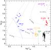 |
Fig. 1 Location of the known ELMVs (big red circles) along with the other several classes of pulsating WD stars (dots of different colors) in the log Teff−log g plane. In parenthesis we include the number of known members of each class. Two post-VLTP (very late thermal pulse) evolutionary tracks for H-deficient WDs and two evolutionary tracks for low-mass He-core WDs are plotted for reference. Also shown is the theoretical blue edge of the instability strip for the GW Vir stars (Córsico et al. 2006), the hot DAV stars, (Shibahashi 2013), V777 Her stars (Córsico et al. 2009a), the DQV stars (Córsico et al. 2009b), the ZZ Ceti stars (Fontaine & Brassard 2008), and the pulsating low-mass WDs (Hermes et al. 2013a). |
The classification of ELMV stars as a new, separate class of pulsating WDs is a matter of debate. On one hand, some authors (e.g., Van Grootel et al. 2013) consider the ELMVs as genuine ZZ Ceti stars but with very low masses. This conception is based on the fact that for both kinds of objects (which share the same spectroscopic classification as DA objects), the pulsations are excited by the same driving κ−γ mechanism associated with the H partial ionization zone. However, there are significant differences between both types of stars. From the point of view of their origin and formation, the low-mass WD stars (including ELM WDs) seem to come from interacting binary evolution and should harbor cores made of unprocessed He. This is in contrast to the case of average-mass ZZ Cetis, which according to the standard evolutionary theory, are the result of single-star evolution and must have cores made of C and O. In addition, that so many constant (non variable) low-mass WDs coexist with ELMV WDs in the same domain of Teff and log g2 may be indicating substantially different internal structures, and so have quite distinct evolutionary origins. This contrasts with the well-documented purity of the ZZ Ceti instability strip, which indicates that all the DA WDs crossing the effective temperature interval 12 500 K ≳ Teff ≳ 10 700 K do pulsate. Another distinctive feature of ELMVs is the length of their pulsation periods, which largely exceed ~ 1200 s and reach up to ~ 6300 s, which is much longer than the periods found in ZZ Ceti stars (100 s ≲ Π ≲ 1200 s). Indeed, the period at Π = 6235 s detected in the ELMV SDSS J222859.93+362359.6 (Hermes et al. 2013a) is the longest period ever measured in a pulsating WD star.
On the theoretical side, the pulsation analysis by Córsico & Althaus (2014a) presently constitutes the most detailed and exhaustive investigation of the adiabatic properties of low-mass WDs. The background equilibrium models employed by those authors were extracted from the complete set of evolutionary sequences of low-mass He-core WD models presented in Althaus et al. (2013). The results of Córsico & Althaus (2014a) (see also the pioneering works of Steinfadt et al. 2010; Córsico et al. 2012) indicate that g modes in ELMVs are restricted mainly to the core regions and p modes to the envelope, providing the chance to constrain both the core and envelope chemical structure of these stars via asteroseismology. On the other hand, nonadiabatic studies (Córsico et al. 2012; Van Grootel et al. 2013) predict that many unstable g and p modes are excited by the same partial ionization mechanism at work in ZZ Ceti stars, roughly at the right effective temperatures and the correct range of the periods observed in ELMVs.
In this paper, our second work of the series on this topic, we perform a thorough stability analysis on the set of state-of-the-art evolutionary models of Althaus et al. (2013). Preliminary results of this analysis were presented in the work of Córsico & Althaus (2014b), which is focused mainly on the role that stable H burning has in destabilizing low-order g modes of ELM WD models. The results of that paper constitute the first theoretical evidence of pulsation modes excited by the ε mechanism in cool WD stars. Here, we extend that analysis by assessing the vibrational stability of radial (ℓ = 0) and nonradial (ℓ = 1,2) p and g modes for the complete set of 14 evolutionary sequences of Althaus et al. (2013) with masses in the range 0.1554−0.4352 M⊙, considering both the κ−γ and ε mechanisms of mode driving and including different prescriptions of the MLT theory of convection.
The paper is organized as follows. In Sect. 2 we briefly describe our numerical tools and the main ingredients of the evolutionary sequences we employ to assess the nonadiabatic pulsation properties of low-mass He-core WDs. In Sect. 3 we present our pulsation results in detail. Section 4 is devoted to comparing the predictions of our nonadiabatic models with the ranges of excited periods in the observed stars. Finally, in Sect. 5 we summarize the main findings of the paper.
2. Computational tools and stellar models
2.1. Evolutionary code
The evolutionary WD models employed in our pulsational analysis were generated with the LPCODE evolutionary code, which produces complete and detailed WD models incorporating very updated physical ingredients in detail. In addition, LPCODE computes the full evolutionary stages leading to the WD formation, allowing study of the WD evolution in a consistent way with the expectations of the evolutionary history of progenitors. While detailed information about LPCODE can be found in Althaus et al. (2005, 2009, 2013) and references therein, we list below only those ingredients that are relevant for our analysis of low-mass, He-core WD stars:
-
The standard mixing length theory (MLT) for convection in the versions ML1, ML2, and ML3 is used. The ML1 version from Böhm-Vitense (1958) has α = 1 and coefficients a = 1/8,b = 1/2,c = 24. The parameter α is the mixing length in units of the local pressure scale height, and the coefficients a,b,c appear in the equations for the average speed of the convective cell, the average convective flux, and the convective efficiency (see Cox 1968). The ML2 version, in turn, comes from Bohm & Cassinelli (1971) and also has α = 1, but coefficients a = 1,b = 2, and c = 16. Finally, the ML3 version is characterized by α = 2 and the same coefficients a,b, and c as in ML2. Physically, the main difference between these different prescriptions of MLT is the increasing convective efficiency going from ML1 to ML3 (for details, see Tassoul et al. 1990).
-
Metallicity of the progenitor stars has been assumed to be Z = 0.01.
-
Radiative opacities for arbitrary metallicity in the range from 0 to 0.1 are from the OPAL project (Iglesias & Rogers 1996). At low temperatures, we use the updated molecular opacities with varying C/O ratios computed at Wichita State University (Ferguson et al. 2005) and presented by Weiss & Ferguson (2009).
-
Conductive opacities are those of Cassisi et al. (2007).
-
The equation of state during the main sequence evolution is that of OPAL for H- and He-rich composition.
-
Neutrino emission rates for pair, photo, and bremsstrahlung processes have been taken from Itoh et al. (1996), and for plasma processes we included the treatment of Haft et al. (1994).
-
For the WD regime we employed an updated version of the Magni & Mazzitelli (1979) equation of state.
-
The nuclear network takes 16 elements and 34 thermonuclear reaction rates for pp-chains, CNO bi-cycle, He burning, and C ignition into account.
-
Time-dependent diffusion due to gravitational settling and chemical and thermal diffusion of nuclear species has been taken into account following the multicomponent gas treatment of Burgers (1969).
-
Abundance changes were computed according to element diffusion, nuclear reactions, and convective mixing. This detailed treatment of abundance changes by different processes during the WD regime constitutes a key aspect in the evaluation of the importance of residual nuclear burning for the cooling of low-mass WDs.
-
For the WD regime and for effective temperatures lower than 10 000 K, outer boundary conditions for the evolving models are derived from nongray model atmospheres (Rohrmann et al. 2012).
2.2. Pulsation code
We carried out our pulsation analysis of radial (ℓ = 0) and nonradial (ℓ = 1,2) p and g modes, employing the nonadiabatic versions of the LP-PUL pulsation code described in detail in Córsico et al. (2006). For the nonradial computations, the code solves the sixth-order complex system of linearized equations and boundary conditions as given by Unno et al. (1989). For the case of radial modes, LP-PUL solves the fourth-order complex system of linearized equations and boundary conditions according to Saio et al. (1983) with the simplifications of Kawaler (1993). Our nonadiabatic computations rely on the frozen-convection (FC) approximation, in which the perturbation of the convective flux is neglected. While this approximation is known to give unrealistic locations of the g-mode red edge of the ZZ Ceti instability strip, it leads to satisfactory predictions for the location of the blue edge (Van Grootel et al. 2012) (see also Saio 2013, for an enlightening discussion of this topic).
2.3. Model sequences
Selected properties of our He-core WD sequences (final cooling branch) at Teff ≈ 10 000 K: the stellar mass, the mass of H in the outer envelope, the time it takes the WD models to cool from Teff ≈ 10 000 K to ≈ 8000 K, and the occurrence (or not) of CNO flashes on the early WD cooling branch.
Stellar parameters (derived using 1D and 3D model atmospheres) and observed pulsation properties of the seven known ELMV stars.
Althaus et al. (2013) derived realistic configurations for low-mass He-core WDs by mimicking the binary evolution of progenitor stars. Full details about this procedure are given in Althaus et al. (2013) and Córsico & Althaus (2014a). Binary evolution was assumed to be fully nonconservative, and the loss of angular momentum owing to mass loss, gravitational wave radiation, and magnetic braking was considered. All of the He-core WD initial models were derived from evolutionary calculations for binary systems consisting of an evolving main sequence low-mass component of initially 1 M⊙ and a 1.4 M⊙ neutron star as the other component. A total of 14 initial He-core WD models with stellar masses between 0.1554 and 0.4352 M⊙ were computed for initial orbital periods at the beginning of the Roche lobe phase in the range 0.9 to 300 d. In Table 1, we provide some relevant characteristics of the whole set of He-core WD models. The evolution of these models was computed down to the range of luminosities of cool WDs, including the stages of multiple thermonuclear CNO flashes during the beginning of cooling branch. Column 1 of Table 1 shows the resulting final stellar masses (M⋆/M⊙). The second column corresponds to the total amount of H contained in the envelope (MH/M⋆) at Teff ≈ 10 000 K (at the final cooling branch), and Col. 3 displays the time spent by the WD models to cool from Teff ≈ 10 000 K to ≈ 8000 K. Finally, Col. 4 indicates the occurrence (or not) of CNO flashes on the early WD cooling branch. There is a threshold in the stellar mass value (at ~ 0.18 M⊙), below which CNO flashes on the early WD cooling branch are not expected to occur, in agreement with previous studies (Sarna et al. 2000; Althaus et al. 2001; Nelson et al. 2004). Sequences with M⋆ ≲ 0.18 M⊙ have thicker H envelopes and much longer cooling timescales than sequences with stellar masses above that mass threshold. To put this in numbers, the H content and τ (the time to cool from Teff ≈ 10 000 K to Teff ≈ 8000 K) for the sequence with M⋆ = 0.1762 M⊙ are ~ 4 and ~ 22 times larger, respectively, than for the sequence with M⋆ = 0.1806 M⊙ (see Table 1). In this example, we are comparing the properties of two sequences with virtually the same stellar mass (ΔM⋆ ≈ 4 × 10⁻³M⊙). The slow evolution of the nonflashing sequences is caused by the residual H burning being the main source of surface luminosity, even at very advanced stages of evolution. We show in Fig. 2 the complete set of evolutionary tracks (final cooling branches) of our low-mass He-core WDs, along with the seven ELMVs discovered so far. We include the location of ELMV stars with Teff and log g values derived from 1D model atmospheres (large red circles), as well as for the case in which these parameters are corrected for 3D effects (small black circles) following Tremblay et al. (2015). These parameters are shown in Table 2. The corrected effective temperatures and gravities are extracted directly from Tremblay et al. (2015), except for the star SDSS J1618+3854, for which we use the fitting functions given by those authors. Visibly, 3D corrections lower the estimated 1D Teff and log g, implying lower masses (compare Cols. 4 and 7 of the table).
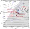 |
Fig. 2 Teff−log g plane showing the low-mass He-core WD evolutionary tracks (final cooling branches) of Althaus et al. (2013). Numbers correspond to the stellar mass of each sequence. The locations of the seven known ELMVs (Hermes et al. 2012, 2013b,a; Kilic et al. 2015; Bell et al. 2015) are marked with large red circles (Teff and log g computed with 1D model atmospheres) and small black circles (after 3D corrections). Stars observed not to vary (Steinfadt et al. 2012; Hermes et al. 2012, 2013b,a) are depicted with hollow small blue circles. The hollow square on the evolutionary track of M⋆ = 0.1762 M⊙ indicates the location of the template model analyzed in Sect. 3. The gray-shaded region bounded by the dashed blue line corresponds to the instability domain of ℓ = 1g modes according to nonadiabatic computations using ML2 (α = 1.0) version of the MLT theory of convection; see Sect. 3.2. |
3. Stability analysis
We analyze the stability pulsation properties of about 7000 stellar models of He-core, low-mass WDs corresponding to a total of 42 evolutionary sequences that include three different prescriptions for the MLT theory of convection (ML1, ML2, ML3; see Tassoul et al. 1990) and covering a range of effective temperatures of 13 000 K ≲ Teff ≲ 6 000 K and a range of stellar masses of 0.1554 ≲ M⋆/M⊙ ≲ 0.4352. For each model, we assessed the pulsation stability of radial (ℓ = 0) and nonradial (ℓ = 1,2) p and g modes with periods from a range 10 s ≤ Π ≤ 18 000 s for the sequence with M⋆ = 0.1554 M⊙, up to a range of periods of 0.3 s ≤ Π ≤ 5000 s for the sequence of with M⋆ = 0.4352 M⊙. Certainly, these ranges of periods are extremely wide when compared to the range of periods observed in ELMVs so far (100 s ≤ Π ≤ 7000 s). The reason for considering such wide ranges of periods in our computations is to clearly define the theoretical domain of instability, that is, to find the long- and short-period edges of the instability domains for all the stellar masses and effective temperatures.
We start by discussing the stability properties of a template 0.1762M⊙ low-mass He-core WD model with Teff = 9500 K and ML2 (α = 1.0). Its location in the Teff−log g diagram is displayed in Fig. 2 as a hollow square. These properties are qualitatively the same for all the models of our complete set of evolutionary sequences. The normalized growth rate η (≡−ℑ(σ)/ℜ(σ), where ℜ(σ) and ℑ(σ) are the real and the imaginary parts, respectively, of the complex eigenfrequency σ) in terms of pulsation periods Π for overstable ℓ = 0,1, and 2 modes corresponding to the selected model is shown in Fig. 3. We note that η> 0 (η< 0) implies unstable (stable) modes. The range of periods of unstable p modes does not depend on the harmonic degree, unlike what happens in the case of g modes, for which the period interval of unstable modes for ℓ = 2 is shifted to shorter periods when compared with the range of ℓ = 1 unstable mode periods. For radial modes and p modes, the growth rate reaches a maximum value (ηmax ~ 4 × 10⁻⁵) in the vicinity of the short-period edge of the instability domain. In other words, within a given band of unstable modes, the excitation is markedly stronger for modes characterized by short periods (high frequencies). The opposite holds for g modes, for which the greatest excitation (ηmax ~ 4.6 × 10⁻³) corresponds to the long-period boundary of the domain of unstable modes. Radial modes and p modes with increasing periods (decreasing radial order k) are all unstable, even the lowest order modes, although with the minimum excitation value (ηmin ~ 10-10). Something quite different occurs in the case of g modes. Specifically, the value of η for g modes gradually decreases for decreasing periods, until it reaches negative values for modes with k = 3,4,5, and 6, which are pulsationally stable. However, modes with k = 1 and 2 are again unstable, although with very low growth rates (η ~ 10-13). In the case of ℓ = 2, even the f mode (k = 0) is unstable, as is clearly documented in Fig. 3. As we discuss below, stable nuclear burning of H plays a role in destabilizing these low-order g modes (k = 1,2), aside from the strong driving associated to the partial ionization of H.
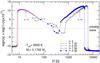 |
Fig. 3 Normalized growth rates η (symbols connected with continuous lines) for radial (ℓ = 0) and nonradial ℓ = 1,2p and g modes in terms of the pulsation periods for the 0.1762 M⊙ ELM WD template model at Teff = 9500 K. The wide numerical range spanned by η is appropriately scaled for a better graphical representation. Specific modes (mode p with ℓ = 1,k = 10 and mode g with ℓ = 1,k = 30), which are analyzed in Fig. 4, are indicated with arrows. |
We have selected two representative unstable pulsation modes of the template model in order to investigate the details of the driving/damping process. Specifically, we chose two overstable dipole (ℓ = 1) modes, one of them a g mode with k = 30 and the other one a p mode with k = 10 (arrows in Fig. 3). In the upper (lower) panel of Fig. 4 we display the differential work function dW/ dr and the running work integral W (see Lee & Bradley 1993, for a definition) for the unstable g mode (p mode), characterized by Π = 2817 s, η = 1.6 × 10⁻⁵ (Π = 19.07 s, η = 1.1 × 10⁻⁵). The scales for dW/ dr and W are arbitrary. Also shown are the Rosseland opacity (κ) and its derivatives (κT + κρ/ (Γ3−1)) and the logarithm of the thermal timescale (τth). We restrict the figure to the envelope region of the model, where the main driving and damping occurs. The region that destabilizes the modes (where dW/ dr> 0) is clearly associated with the bump in the opacity owing to the ionization of H at the outer convection zone (gray area in the figure), centered at −log q ~ 12[q ≡ (1−Mr/M⋆)], although the maximum driving comes from a slightly more internal regions (−log q ~ 11.5 for the g mode and −log q ~ 11.0 for the p mode). The thermal timescale reaches values in the range 103−104 s at the driving region, compatible with the longest excited period of the template model, at ~ 6200 s. In the driving region, the quantity κT + κρ/ (Γ3−1) is increasing outward, in agreement with the well known necessary condition for mode excitation (Unno et al. 1989). For the g mode, the contributions to driving at −log q from ~ 11 to ~ 12 largely overcome the weak damping effects at −log q ≲ 11 and −log q ≳ 12, as reflected by the fact that W> 0 at the surface, and so the mode is globally excited. Similarly, the strong driving experienced by the p mode (denoted by positive values of dW/ dr for 11 ≲ −log q ≲ 11.5) makes this mode globally unstable.
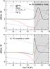 |
Fig. 4 Differential work (dW/ dr) and the running work integral (W) for the g mode with k = 30 (upper panel) and the p mode with k = 10 (lower panel), along with the Rosseland opacity profile (κ), the opacity derivatives, and the thermal timescale (τth) of our 0.1762 M⊙ ELM WD template model (Teff = 9500 K). The gray area shows the location of the outer convection zone. |
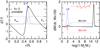 |
Fig. 5 Left panel: Lagrangian perturbation of temperature (δT/T), along with the scaled nuclear generation rate (ϵ) and the H and He chemical abundances (XH,XHe) in terms of the normalized stellar radius, for the unstable ℓ = 1,k = 2g mode (Π = 325 s) corresponding to our template model. The black dot marks the location of the outermost maximum of δT/T. Right panel: corresponding differential work function (dW/ dr) in terms of the mass fraction coordinate for the case in which the ε mechanism is allowed to operate (solid black curve) and when it is suppressed (solid red curve). Also shown are the scaled running work integrals, W (dotted curves). |
3.1. The destabilizing role of H burning
Córsico & Althaus (2014b) have explored the impact of stable H burning on the pulsational stability properties of the same models of low-mass He-core WDs analyzed here. They found that, besides a dense spectrum of unstable radial modes and nonradial g and p modes driven by the κ−γ mechanism due to the partial ionization of H in the stellar envelope, some unstable g modes with short pulsation periods are also destabilized by H burning via the ε mechanism (Unno et al. 1989) of mode driving. Córsico & Althaus (2014b) speculate that the short periods at Π ~ 108 s and Π ~ 134 s detected in the ELMV star SDSS J1112+1117 (Hermes et al. 2013b) could be excited by this mechanism. If true, this could constitute the first evidence of the existence of stable H burning in cool WD stars. These interesting results rely, however, on the reality of those short pulsation periods, something that needs additional observations to be confirmed (J. J. Hermes, priv. comm.).
To show how the ε mechanism acts to destabilize low-order g modes in our models, we restrict the description to the k = 2 mode of our selected template model. This mode is unstable, with η = 4.76 × 10⁻¹⁴. Admittedly, this growth rate is extremely low, and one can wonder if this mode, being marginally unstable, is able to reach amplitudes large enough to be observable. To answer that question we have to examine the e-folding time, defined as τe = 1/ | ℑ(σ) |. For this mode, τe = 3.44 × 10⁷ yr. This is an estimate of the time it would take the mode to reach amplitudes large enough to be observable. It has to be compared with the evolutionary timescale (τ), which represents the time that the model spends evolving in the regime of interest. In this case, we have τ ~ 7.6 × 10⁹ yr3. Since τe ≪ τ, we conclude that the mode has plenty of time to develop large amplitudes while the star is slowly cooling at that effective temperature regime.
To assess the role that stable H burning has in the destabilization of the k = 2g mode of the template model, we redid the stability computations, but this time suppressing the action of this destabilizing agent. Specifically, we force the nuclear energy production rate, ϵ, and their logarithmic derivatives ϵT = (∂lnϵ/∂lnT)ρ and ϵρ = (∂lnϵ/∂lnρ)T to be zero in the pulsation equations. The results are shown in the righthand panel of Fig. 5, which shows the differential work function (dW/ dr) in terms of the mass fraction coordinate for the case in which the ε mechanism is allowed to operate (solid black curve) and when it is suppressed (solid red curve). Also shown are the scaled running work integrals, W (dotted curves). The lefthand panel of the figure displays the Lagrangian perturbation of temperature, δT/T. The peak of the (scaled) nuclear generation rate ϵ at r/R⋆ ~ 0.50 marks the location of the H-burning shell at the He/H chemical interface. We emphasize the position of the outermost maximum of δT/T with a black dot. The ε mechanism behaves as an efficient filter of modes that provides substantial driving only to those g modes that have their maximum of δT/T in the narrow region of the burning shell (Kawaler et al. 1986). The g mode with k = 2 met this condition.
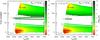 |
Fig. 6 Left panel: unstable ℓ = 1 mode periods (Π) in terms of the effective temperature, corresponding to the ELM WD model sequence with M⋆ = 0.1762 M⊙. Color coding indicates the value of the logarithm of the e-folding time (τe) of each unstable mode (right scale). The vertical line indicates the effective temperature of the template model analyzed in Fig. 3. Right panel: same as left panel, but for the case in which the action of the ε mechanism is neglected in the stability computations. |
In the case where the ε mechanism is taken into account, there is appreciable driving (dW/ dr> 0) at the region of the H-burning shell (−log q ~ 2), as can be appreciated from the righthand panel of Fig. 5. The destabilizing effect of nuclear burning adds up to the excitation due to the H partial ionization at the envelope (−log q ~ 11), and the mode is globally unstable. Both contributions of driving are also visible as positive slopes of the work integral at those locations of the model. When we suppress the ε mechanism (red curves), strong damping takes place in the region of the burning shell. In this case, the driving due to the H partial ionization at the envelope is not able to overcome the damping in that region, and the mode turns out to be pulsationally stable. We can conclude that for this specific model, the g mode with k = 2 is globally unstable thanks to the destabilizing effect of the H-burning shell through the ε mechanism.
A more general and comprehensive perspective of the role of the ε mechanism in our pulsation models can be achieved by examining the properties of our template model for the full range of effective temperatures. In the lefthand panel of Fig. 6, we show the instability domain of ℓ = 1 periods in terms of the effective temperature for the ELM WD model sequence with M⋆ = 0.1762 M⊙. The palette of colors (righthand scale) indicates the value of the logarithm of the e-folding time (in years) of each unstable mode. As can be seen, many unstable pulsation modes exist, which are clearly grouped in the two families, one of them corresponding to long periods and associated with g modes, and the other one characterized by short periods and belonging to p modes. Most of these modes are destabilized by the κ−γ mechanism acting at the surface H partial ionization zone. The strongest excitation, that is, the shortest e-folding time (light red and yellow zones), is found for high-order g and p modes, with periods in the ranges 3000−10 000 s and 7−30 s, respectively, and effective temperatures near the hot boundary of the instability islands (Teff ~ 9600−9800 K). Although with shorter unstable g-mode periods (2000−10 000) s, similar results are obtained for ℓ = 2 (not shown). The righthand panel of Fig. 6 shows the results of our stability computations when we shut down the ε mechanism. Interestingly enough, the k = 2 and k = 3g modes become stable for the complete range of effective temperatures analyzed, and they do not appear in this plot. Something similar happens with the modes with k = 1, k = 4, and k = 6 in certain ranges of Teff. We can conclude that these modes are excited to a great extent by the ε mechanism through the H-burning shell. We note that high-order g modes are insensitive to the effects of nuclear burning, and the same holds for the complete spectrum of p modes and radial modes.
Stellar mass, the mass of H, the evolutionary timescale, the radial order and harmonic degree, the Teff-range of instability, the average period, the maximum e-folding time, and the ratio of the evolutionary timescale to the maximum e-folding time, corresponding to unstable short-period ℓ = 1,2g modes for which the ε mechanism strongly contributes to their destabilization, corresponding to model sequences with M⋆ ≤ 0.2389 M⊙ computed using the ML2 prescription of the MLT theory of convection.
In Table 3 we present the short-period ℓ = 1,2g modes for which the ε mechanism strongly contributes to their destabilization, corresponding to sequences with stellar masses below 0.2389 M⊙. The number of ε-destabilized modes is larger for sequences with masses ≤ 0.1762 M⊙, by virtue of these models having thick H envelopes, and as a result, they are able to sustain an intense H nuclear burning. For models with M⋆ ≥ 0.1806 M⊙, nuclear burning is much weaker, but still able to contribute to the driving of g modes with radial order k = 1,2. We note, however, that in the case of models with M⋆ = 0.1863 M⊙ and M⋆ = 0.1917 M⊙, the e-folding times are shorter than the evolutionary timescale with ratios  . Although formally unstable, these modes do not have enough time as to reach observable amplitudes while the star is crossing the Teff interval 10 000−8000 K. For masses above 0.2389 M⊙ (not shown), only modes with ℓ = 1,2 and k = 1 are ε-destabilized modes.
3.2. Characterizing the blue edge of the theoretical ELMV instability strip
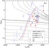 |
Fig. 7 Teff−log g diagram showing the blue edge of the ELMV instability domain for the cases of radial modes (black solid line), nonradial dipole g modes (solid red line), nonradial quadrupole g modes (dashed red lines), and nonradial dipole and quadrupole p modes (blue solid line), for the case where stellar models are computed using the ML2 version of the MLT theory. The known ELMVs are also depicted. Filled red circles correspond to the location of the stars using 1D model atmospheres, filled black circles indicate their location according to 3D model atmospheres, and hollow blue circles are associated with low-mass WDs that are observed not to vary. |
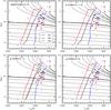 |
Fig. 8 Teff−log g diagrams displaying our low-mass He-core WD evolutionary tracks along with the blue (hot) edge of the ELMV instability strip for radial (ℓ = 0) and nonradial (ℓ = 1,2) p and g modes, corresponding to different versions of the MLT theory of convection: ML1 (blue), ML2 (black), and ML3 (red). Again, the known ELMVs and the stars observed not to vary are also depicted. In the case of ℓ = 1g modes, we have included the blue edges computed with the TDC treatment (dashed black line) and the FC approximation (dot dashed black line), and also the red edge (dotted black line) of the instability strip from Van Grootel et al. (2013). |
Here, we examine the location of the instability domains of our low-mass He-core WDs for radial and nonradial g and p modes on the Teff−log g plane. The locus of the blue (hot) edge of instability is illustrated in Fig. 7 for the case where the surface convection in the equilibrium models is treated according to the ML2 (α = 1) version of the MLT theory. A note about the way in which the blue edge is defined in this work is in order. Generally, as the models of our evolutionary sequences cool, the first g modes to became unstable are those of low radial order (k = 1,2). In most cases, the ε mechanism plays a crucial role in the destabilization of these modes (see Figs. 5 and 6). At some lower Teffs, higher order modes (k = 6,7,8,...) are destabilized, while intermediate-order modes (k = 3,4,5) remain pulsationally stable at those effective temperatures (Fig. 6). This is particularly notorious in our less massive (M⋆ ≤ 0.1762 M⊙) sequences. In defining the blue edge of instability for g modes, therefore, we adopt the effective temperature at which the bulk of modes (k ≳ 6) become unstable4. In the case of radial modes and nonradial p modes, there is no ambiguity since these modes are destabilized gradually, starting from the lowest radial orders (k = 0,1,2,3,... for radial modes and k = 1,2,3,... for p modes).
Figure 7 shows that the blue edges associated to radial modes and nonradial p modes are ~ 200 K hotter than those corresponding to g modes. This means that radial modes and nonradial p modes are first destabilized as the models cool, as can be clearly appreciated from Fig. 6. We also found that the blue edge of radial modes is slightly cooler than for the p modes and that the blue edge for the p modes is largely independent of the harmonic degree. On the other hand, the blue edge of g modes is weakly sensitive to the ℓ value, because it is up to ~ 45 K hotter for ℓ = 2 than for ℓ = 1.
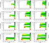 |
Fig. 9 Unstable mode periods (Π) for ℓ = 0 (left panels), ℓ = 1 (middle panels), and ℓ = 2 (right panels) in terms of the effective temperature, corresponding to the ELM WD model sequences constructed using the ML2 version of the MLT theory of convection and with stellar masses (from top to bottom) M⋆ = 0.1554 M⊙, M⋆ = 0.1762 M⊙, M⋆ = 0.1805 M⊙, and M⋆ = 0.4352 M⊙. Color coding indicates the value of the logarithm of the e-folding time (τe) of each unstable mode (right scale). |
The dependence of the blue edges of instability on the convective efficiency adopted in the equilibrium models is documented in Fig. 8, where we show the Teff−log g diagrams displaying our low-mass He-core WD evolutionary tracks, along with the blue (hot) edge of the ELMV instability strip for radial (ℓ = 0) and nonradial (ℓ = 1,2) p and g modes, which correspond to different versions of the MLT theory of convection: ML1 (blue), ML2 (black), and ML3 (red). As expected, the blue edge in the case of the ML3 version is hotter than for the ML2 version, and it is in turn hotter than the ML1 prescription. The shift in the effective temperature of the blue edges for the different versions of the MLT is between ~ 600 K and ~ 1300 K. The main result exhibited by this figure is that only the ML2 and ML3 prescriptions of the MLT actually account for all the observed ELMV stars (filled red and black circles), regardless of whether 3D model atmosphere corrections are considered to estimate Teff and log g. Interestingly, no ELMV is found to be hotter than the blue edge associated to the ML2 version, but it can be due to the small sample of stars.
Our blue edge for ℓ = 1g modes with ML2 is in excellent agreement with the blue edges derived by Van Grootel et al. (2013), shown in the lower lefthand panel of Fig. 8 when there is a time-dependent convection treatment (TDC) and when those authors use the FC approximation. The agreement between our computations and those of Van Grootel et al. (2013) breaks down for masses lower than the limit mass ~ 0.18 M⊙, below which CNO flashes on the early WD cooling branch are not expected to occur. We have also included an estimation for the red edge, as proposed by Van Grootel et al. (2013) (black dotted line). This estimation is based on the atmosphere energy leakage argument elaborated by Hansen et al. (1985). It is apparent that the proposed red edge from Van Grootel et al. (2013) does not describe the observations.
We now explore the ranges of periods of unstable modes and their dependence with stellar mass, the effective temperature, and the version of the MLT theory employed. Figure 9 shows the unstable radial and nonradial p and g modes on the Teff−Π plane for the evolutionary sequences with M⋆/M⊙ = 0.1554,0.1762,0.1805, and 0.4352. The periods of unstable nonradial modes for each sequence are clearly grouped in two separated regions, one of them characterized by short periods and corresponding to p modes, and the other one characterized by long periods and associated to g modes. In the case of radial modes, there is a single instability region with periods very similar to those of the nonradial p modes. In the case of ℓ = 2, there is the f mode in between the regions of p and g modes. The longest excited periods for g modes reach values up to ~ 15 500 s (ℓ = 1) and ~ 10 000 s (ℓ = 2) for the lowest mass sequence (M⋆/M⊙ = 0.1554), and these numbers drastically decrease to ~ 3500 s (ℓ = 1) and ~ 2000 s (ℓ = 2) for the most massive sequence (M⋆/M⊙ = 0.4352). The shortest excited periods, in turn, range from ~ 285 s (ℓ = 1) and ~ 185 s (ℓ = 2) for M⋆/M⊙ = 0.1554, to ~ 135 s (ℓ = 1) and ~ 80 s (ℓ = 2) for M⋆/M⊙ = 0.4352. The longest and shorter excited periods of g modes are longer for lower M⋆ and lower ℓ. In the case of radial modes and nonradial p modes, the shortest excited periods range from ~ 19 s (M⋆/M⊙ = 0.1554) up to ~ 0.5 s (M⋆/M⊙ = 0.4352). Notably, the shortest excited periods of p modes are insensitive to the value of ℓ. On the other hand, the longest excited periods (which also are insensitive to the value of ℓ) go from ~ 160 s (M⋆/M⊙ = 0.1554) to ~ 12 s (M⋆/M⊙ = 0.4352). We conclude that the longest and shortest excited periods of p modes and radial modes are greater for lower M⋆ and they do not depend on ℓ. We did not find any qualitative differences in the characteristics of the instability domains of radial and nonradial p modes, except for a very small shift in the effective temperature of the blue edges, as mentioned before.
Regarding the strength of the mode instability, we found that the most unstable modes (that is, with the shortest e-folding times) are generally those characterized by high radial orders. As for the dependence of the destabilization of modes with Teff, we found that the most unstable pulsation modes correspond to stellar models located near the blue edge of instability. The modes gradually become less unstable as the model cools. All these properties are clearly illustrated in Fig. 9. In the context of our non-adiabatic calculations, which assume the FC approximation, the red edge of the instability domain (that is, the effective temperature at which the pulsations stop) is located at about Teff = 6000−5000 K (not shown in Fig. 9), so much lower than the Teff of the coolest known ELMV star (SDSS J2228+3623, Teff ~ 7900 K). This disagreement cannot be attributed, however, to the use the FC approximation since an identical result is found by Van Grootel et al. (2013) using a TDC treatment (see their Fig. 3)5. Similarly, Van Grootel et al. (2012) find Teff ≲ 6000 K for the red edge of ZZ Ceti stars. Clearly, a missing physical mechanism is at work in real stars that quenches the pulsations at much higher effective temperatures.
Finally, we examined the dependence of the longest and shortest excited periods with the prescription of the MLT theory employed. For sequences with M⋆ ≤ 0.1762 M⊙, we found that the longest excited period of g modes is substantially longer for higher convective efficiency. In particular, in the case of the sequence with M⋆/M⊙ = 0.1554, we found that the longest excited period is ~ 13 600 s for ML1, ~ 15 500 s for ML2, and ~ 17 600 s for ML3. On the other hand, for sequences with M⋆ ≥ 0.1806 M⊙, the trend is the opposite: the longest excited period of g modes is shorter for higher convective efficiency, although the differences are small. For instance, for the sequence with M⋆/M⊙ = 0.4352, we find that the longest unstable period is ~ 3350 s (ML1), ~ 3300 s (ML2), and ~ 3150 s (ML3). Regarding the shortest excited periods for g modes, we do not find an appreciable dependence with the convective efficiency of the models. In the case of p modes and radial modes, we find that the largest and shortest excited periods are fairly insensitive to the version of the MLT employed, having however a weak trend of higher shortest and longest unstable periods with higher convective efficiency.
4. Comparison with the observed ELMVs
Having shown that our theoretical predictions are in good agreement with the position of the ELMVs in the diagram Teff−log g – provided that the stellar models are computed with the ML2 version of the MLT theory of convection – in this section we want to compare the theoretical ranges of periods associated to unstable modes with the pulsation periods exhibited by the observed stars. In Table 2 we show the main spectroscopic data available for the seven ELMV stars known up to now. We include the values of Teff and log g derived from 1D model atmospheres and the stellar mass M⋆ computed from the tracks of Althaus et al. (2013), and also in the case where Teff and log g are corrected by 3D effects, following Tremblay et al. (2015). Here, we first adopt the effective temperatures and gravities of ELMV stars derived from 1D model atmospheres, and next we consider the case where the values are corrected by 3D effects.
It should be noted that, for ELM stars, only Teff and log g can be directly constrained from observations and model atmospheres, and not their stellar mass. To get the mass, it is necessary to assume some evolutionary stage, because many low-mass WD evolutionary tracks overlap at different stages due to the developments of CNO flashes (see Fig. 2 of Althaus et al. 2013). Because of this, the masses of ELMVs could be off by 0.10 M⊙ or more if the ELM WD was experiencing a CNO flash.
4.1. Using Teff and log g derived from 1D model atmospheres
We start by considering the ELMV star SDSS J2228+3623, the coolest and least massive object of the class detected to date (Teff ~ 7900 K and M⋆ ~ 0.15 M⊙). The pulsations of this star were discovered by Hermes et al. (2013a). That this star is so cool compared with the six warmer pulsating ELMVs raises the question of whether this star is an authentic ELMV star or is instead a more massive pre-ELM WD that is looping through the Teff−log g diagram prior to settling on its final WD cooling track (Hermes et al. 2013a). The hypothesis that this star might be a pre-WD is interesting, even if considering that the evolution of the pre-WDs is much faster than that of the ELM WDs, and therefore there are far fewer opportunities of observing it. This issue has been examined by Córsico & Althaus (2014a), but without conclusive results. In Fig. 10 we show the theoretical unstable ℓ = 1 mode periods that correspond to the evolutionary sequence of M⋆ = 0.1554 M⊙, the closest stellar mass of our grid to the mass inferred for this star. We also include the pulsation periods of SDSS J2228+3623 at 3254.5 s, 4178.3 s, and 6234.9 s. The three periods are well accounted for by the theoretical computations. In particular, the longest period (6234.9 s) is quite close to the theoretical upper limit of unstable mode periods at the lower limit of Teff of this star (Πmax ~ 6800 s). For the effective temperatures of interest, g modes are still quite unstable with e-folding times of roughly 103−104 yrs.
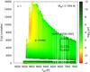 |
Fig. 10 Periods of unstable ℓ = 1 modes in terms of the effective temperature, with the palette of colors (right scale) indicating the value of the logarithm of the e-folding time (in years), corresponding to the sequence with M⋆ = 0.1554 M⊙. Also shown are the pulsation periods of the ELMV star SDSS J2228+3623 (horizontal segments). The adopted value of Teff (and its uncertainties) is the one derived from 1D model atmospheres (see Table 2). The gaps for Teff ≲ 8200 K in the unstable models are due to an insufficiently fine grid. |
The ELMV star SDSS J1614+1912 was also discovered to be pulsating by Hermes et al. (2013a). This star has Teff ~ 8800 K and M⋆ ~ 0.19 M⊙, and it pulsates in just two periods at 1184.1 s and 1262.7 s. These are relatively short periods when compared with the periods detected in the other ELMVs, except SDSS J1112+1117 (see below). This is something striking considering that, as the second coldest known ELMV star (after SDSS J2228+3623), its relatively short periods do not match the well known trend in ZZ Ceti stars of an increase in pulsation periods for lower effective temperatures (Clemens 1993; Mukadam et al. 2006). According to its stellar mass, we have to compare these periods with the theoretical range of unstable mode periods of our sequence with M⋆ = 0.1917 M⊙. This comparison is displayed in Fig. 11. Clearly, both periods are well accounted for by the theoretical computations.
Next, we focus our attention on the ELMV stars SDSS J1518+0658 (Hermes et al. 2013b) and SDSS J1618+3854 (Bell et al. 2015), which have Teff ~ 9900 K and Teff ~ 9140 K , respectively. With a stellar mass of M⋆ ~ 0.22 M⊙ estimated for these two stars, they are the most massive ELMVs known hitherto. We compare the observed periods with the theoretical predictions corresponding to the evolutionary sequences with M⋆ = 0.2019 M⊙ and M⋆ = 0.2389 M⊙, thus embracing the stellar mass derived for both stars. We show the results in Fig. 12. The 13 periods exhibited by SDSS J1518+0658 in the range 1335−3848 s are supported by our nonadiabatic computations. Indeed, the detected periods, particularly those longer than ~ 2000 s, correspond to the most unstable theoretical g modes of the instability domain, characterized by e-folding times in the range 10-2−10-1 yrs. In the case of SDSS J1618+3854, our theoretical computations are successful in reproducing the shortest observed periods at 2543 s and 4935 s, but they fail to predict the existence of the longest one (6125 s). If our nonadiabatic models are a good representatation of ELMVs, we can therefore rule out the masses 0.2019 M⊙ and 0.2389 M⊙ for this star from the exhibited period range alone.
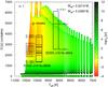 |
Fig. 12 Similar to Fig. 10, but for the the 0.2019 M⊙ and 0.2389 M⊙ sequences and the ELMV stars SDSS J1518+0658 and SDSS J1618+3854. |
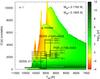 |
Fig. 13 Similar to Fig. 10, but for the the 0.1762 M⊙ and 0.1805 M⊙ sequences and the ELMV stars SDSS J1112+1117, SDSS J1840+6423, and PSR J1738+0333. |
Finally, in Fig. 13 we depict the situation for the remaining three ELMV stars, SDSS J1112+1117 (Hermes et al. 2013b), SDSS J1840+6423 (Hermes et al. 2012), and PSR J1738+0333 (Kilic et al. 2015). These stars have stellar masses M⋆/M⊙ ~ 0.179,0.183, and 0.181, respectively, near the critical mass for the development of CNO flashes (~ 0.18 M⊙). As shown in Córsico & Althaus (2014a), ELM stars in this range of masses can harbor very different internal chemical structures and, in particular, quite distinct H layer thicknesses, which should be reflected in their pulsation spectra. Future asteroseismological analysis of these stars will therefore have the potential to place strong constraints on the previous evolutionary history of their progenitors. We include in Fig. 13 the domains of unstable mode periods corresponding to the sequences with M⋆ = 0.1762M⊙ and M⋆ = 0.1805 M⊙, thus enclosing the masses inferred for the three stars. The figure reveals that the periods measured in these stars are well accounted for by our stability computations.
The case of SDSS J1112+1117 is particularly interesting because this is the only ELMV star that shows short periods (108 s and 134 s), in addition to the long periods (~ 1800−2900 s) typical of the class. Hermes et al. (2013b) propose the possibility that these short periods could be associated to p modes. This idea was examined by Córsico & Althaus (2014a), who found that, in the framework of the models of Althaus et al. (2013), if the temperature and mass (gravity) of the star are correct, the short periods cannot be attributed to p modes or radial modes. Alternatively, Córsico & Althaus (2014b) demonstrate that these short periods can be associated to low-order g modes destabilized mainly by the ε mechanism by stable nuclear burning at the base of the H envelope.
4.2. Using Teff and log g corrected by 3D model atmosphere effects
Here, we assess how well our theoretical computations fit the observations when we adopt the ELMV Teff and log g parameters after 3D corrections as given by Tremblay et al. (2015). The situation for SDSS J2228+3623 does not change, because its effective temperature does not experience a significant shift when 3D corrections are taken into account (ΔTeff ~ 20 K; see Table2), and although the log g shift is large, the mass of the star still is below 0.1554 M⊙. Thus, the comparison already shown in Fig. 10 holds even when we adopt the 3D corrected (Teff,log g) for this star. Since the long-period boundary of the domain of unstable modes is longer for lower stellar masses, we conclude that the theoretical computations are in good agreement with the range of excited periods of SDSS J2228+3623. In the case of SDSS J1840+6423, on the other hand, since the stellar mass is ~ 0.177 M⊙ when we consider 3D corrected parameters (see Fig. 2), the comparison between observed and theoretical ranges of excited periods shown in Fig. 13 is still valid. In particular, the observed range of excited periods is well accounted for by the theoretical computations corresponding to the sequence with M⋆ = 0.1762 M⊙ when the effective temperature of this star shifts from Teff = 9390 K (1D) to Teff = 9120 K (3D).
For the remaining five ELMVs, the Teff, log g and M⋆ change substantially when we correct for 3D effects, and we must make further comparisons. To begin with, in Fig. 14 we show the case of SDSS J1112+1117, in which the observed periods are compared with the excited theoretical periods of the 0.1650 M⊙ and 0.1706 M⊙ sequences. In this case, the Teff turns out to be 350 K lower, and the stellar mass goes from 0.179 M⊙ to 0.169 M⊙, when we take the 3D corrections into account. Clearly, the observed range of periods is reproduced well by the theoretical computations. Interestingly, we found that in this case the shortest periods at 108 s and 134 s could be safely identified with the k = 1p mode of the 0.1650 M⊙ sequence, at variance with the conclusion of Córsico & Althaus (2014a), who considered the Teff and log g derived from 1D model atmospheres.
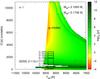 |
Fig. 14 Periods of unstable ℓ = 1 modes in terms of the effective temperature, corresponding to the 0.1650 M⊙ and 0.1706 M⊙ sequences. Also shown are the pulsation periods of the ELMV star SDSS J1112+1117. The Teff adopted for the star is its 1D value corrected by 3D model atmosphere effects (see Table 2). |
In Fig. 15 we illustrate the cases of PSR J1738+0333 and SDSS J1614+1912, where the observed ranges of periods are compared with the theoretical ones corresponding to the sequences with M⋆ = 0.1706 M⊙ and M⋆ = 0.1762 M⊙. Clearly, the observed ranges of excited periods in these stars is accounted for by the theoretical computations.
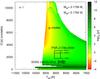 |
Fig. 15 Similar to Fig. 14, but for the case of PSR J1738+0333 and SDSS J1614+1912, and for the 0.1706 M⊙ and 0.1762 M⊙ sequences. |
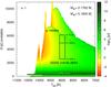 |
Fig. 16 Similar to Fig. 14, but for the case of SDSS J1618+3854 and for the 0.1762 M⊙ and 0.1805 M⊙ sequences. |
The situation for SDSS J1618+3854 is depicted in Fig. 16. The comparison in this case is made with the theoretical unstable modes corresponding to the 0.1762 M⊙ and 0.1805 M⊙ sequences. There is a good agreement between the observations and the theoretical predictions. In particular, the existence of the longest period at 6125 s is reliably predicted by our stability computations. This is at variance with the case in which we adopted the Teff and log g derived from 1D model atmospheres (see Fig. 12). This finding gives strong support to the 3D model atmosphere calculations of Tremblay et al. (2015).
Finally, we display in Fig. 17 the case of SDSS J1518+0658, for which we compare the observed range of periods with the theoretical computations corresponding to the sequences with M⋆ = 0.1917 M⊙ and M⋆ = 0.2019 M⊙. Again in this case our theoretical predictions are in excellent agreement with the range of excited periods observed in the star.
We close this section by noting that for all the analyzed ELMV stars, the number of periods detected is disappointingly low in comparison with the rich spectrum of periods of unstable modes, which include radial and nonradial p and g modes, as predicted by theoretical computations. As for the other classes of pulsating WDs, there must be some unknown filter mechanism present in real stars that favors only a few periods (out of the available dense spectrum of eigenmodes) to reach observable amplitudes. Finding that missing piece of physics in our pulsation models is beyond the scope of the present paper.
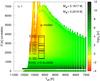 |
Fig. 17 Similar to Fig. 14, but for the case of SDSS J1518+0658, and the 0.1917 M⊙ and 0.2019 M⊙ sequences. |
5. Summary and conclusions
In this paper, we have presented a detailed pulsation stability study of pulsating low-mass WDs employing the set of state-of-the-art evolutionary models of Althaus et al. (2013). This is the second paper in a series on this topic, with the first one focused on the adiabatic properties of low-mass WDs (Córsico & Althaus 2014a). Preliminary results of the nonadiabatic analysis detailed here have already been presented in Córsico & Althaus (2014b), which focused on the role that stable H burning has in destabilizing low-order g modes of ELM WD models. In the present paper, we extend that analysis by assessing the pulsational stability of radial (ℓ = 0) and nonradial (ℓ = 1,2) g and p modes for the complete set of 14 evolutionary sequences of the low-mass He-core WD models of Althaus et al. (2013) with masses in the range 0.1554−0.4352 M⊙, considering both the κ−γ and ε mechanisms of mode excitation and including different prescriptions of the MLT theory of convection.
Our main findings are summarized below:
-
For all the model sequences analyzed, a dense spectrum of unstable radial modes and nonradial g and p modes are excited by the κ−γ mechanism due to the H partial ionization zone in the stellar envelope. In addition, some short-period g modes are destabilized mainly by the ε mechanism due to stable nuclear burning at the basis of the H envelope (Fig. 6), particularly for model sequences with M⋆ ≲ 0.18 M⊙ (see Table 3).
-
The blue edge of the instability domain in the Teff−log g plane is hotter the higher the stellar mass and convective efficiency (Fig. 7). The ML2 and ML3 versions of the MLT theory of convection are the only ones that correctly account for the location of the seven known ELMV stars, regardless of whether the Teff and log g for the stars are derived from standard 1D model atmospheres or if these parameters are corrected by 3D effects (see Fig. 8). There is no dependence of the blue edge of p modes on the harmonic degree; in the case of g modes, we found a weak sensitivity of the blue edge with ℓ. Finally, the blue edges corresponding to radial and nonradial p modes are somewhat (~ 200 K) hotter than the blue edges of g modes.
-
Generally, the most unstable modes (shorter e-folding times) are those characterized by high and intermediate radial orders. For instance, in the case of the sequence with M⋆ = 0.1762 M⊙ and ML2, the most unstable modes have periods between ~ 2000 s and ~ 10 000 s (k between ~ 20 and ~ 110) for g modes, and periods between ~ 7 s (k = 35) and ~ 30 s (k = 7) for p modes and radial modes. The most unstable modes correspond to stellar models located near the blue edge of the instability domain (see Fig. 9).
-
The longest and shorter excited periods of g modes are longer for lower M⋆ and lower ℓ. In the case of p modes and radial modes, the longest and shortest excited periods are longer for lower M⋆, although they do not depend on ℓ.
-
For sequences with M⋆ ≤ 0.1762 M⊙, the longest excited periods of g modes are substantially longer for higher convective efficiency. On the contrary, for M⋆ ≥ 0.1805 M⊙ the longest excited periods of g modes are shorter for higher convective efficiency, although the differences are small. In the case of p modes and radial modes, we found a very weak trend toward longer shortest and longest unstable periods with higher convective efficiency.
-
We compared the ranges of unstable mode periods predicted by our stability analysis with the ranges of periods observed in the ELMV stars. Irrespective of whether we adopt the (Teff,log g) derived from 1D model atmospheres or these parameters corrected by 3D effects, we generally found excellent agreement, as shown by Figs. 10 to 17.
-
In the specific case of SDSS J1618+3854, if we adopt Teff and log g as derived from 1D model atmosphere computations, our nonadiabatic models are unable to explain the existence of the longest period at 6125 s (Fig. 12). However, this period is reliably predicted when we adopt Teff and log g values corrected by 3D model atmosphere effects (Fig. 16). This gives strong support to the 3D model atmospheres of Tremblay et al. (2015).
The results of this study, along with those of previous research (Steinfadt et al. 2010; Córsico et al. 2012; Van Grootel et al. 2013; Córsico & Althaus 2014b), allow us to know the origin and basic nature of the pulsations exhibited by ELMV stars. However, even though theoretical models reproduce the observations qualitatively, some essential unknowns still remain. For instance, there is the problem of the red edge of the instability strip. Our calculations, which assume the FC approximation, as well as those of Van Grootel et al. (2013), which include a TDC treatment, predict a red edge that is extremely cool (Teff ~ 5000−6000 K) as compared with the coolest ELMV star (SDSS J2228+3623, Teff ~ 7900 K). Fortunately, this incomplete knowledge of the physics of WD pulsations does not prevent us from moving forward in asteroseismological studies based on adiabatic calculations, in which the physical agent that drives the pulsations does not matter, but the value of the periods themselves do matter, and they depend sensitively on the internal structure of the WD star. Asteroseismological analysis will provide valuable clues to the internal structure and evolutionary status of low-mass WDs, allowing us to place constraints on the binary evolutionary processes involved in their formation. But to extend the parameter space to explore, we have to consider a possible range of H envelope thicknesses. We plan to compute new evolutionary sequences of low-mass He-core WDs with different angular-momentum loss prescriptions due to mass loss, which could have an impact on the final H envelope mass. Results of these investigations will be presented in an upcoming paper.
For simplicity, here and throughout the paper we refer to the pulsating low-mass WDs as ELMVs, even in the cases in which M⋆ ≳ 0.18−0.20 M⊙.
That is, the domain of instability seems to not be “pure” (Hermes et al. 2013a).
More precisely, this is the time that the template model takes to cool from Teff ~ 10 000 K to ~ 8000 K.
If, instead, we were adopting the Teff at which modes with k = 1,2 become unstable, then the blue edges would be somewhat hotter.
This red edge, which emerges from the nonadiabatic computations of Van Grootel et al. (2013), should not be confused with the estimation of the red edge carried out by the same authors on the basis of the atmosphere energy leakage argument (Fig. 8).
Acknowledgments
We wish to thank our anonymous referee for the constructive comments and suggestions that greatly improved the original version of the paper. We warmly thank K. J. Bell and J. J. Hermes for reading the paper and making enlightening comments and suggestions. Part of this work was supported by AGENCIA through the Programa de Modernización Tecnológica BID 1728/OC-AR, and by the PIP 112-200801-00940 grant from CONICET. This research made use of NASA Astrophysics Data System.
References
- Althaus, L. G., Serenelli, A. M., & Benvenuto, O. G. 2001, MNRAS, 323, 471 [NASA ADS] [CrossRef] [Google Scholar]
- Althaus, L. G., Serenelli, A. M., Panei, J. A., et al. 2005, A&A, 435, 631 [NASA ADS] [CrossRef] [EDP Sciences] [Google Scholar]
- Althaus, L. G., Panei, J. A., Romero, A. D., et al. 2009, A&A, 502, 207 [NASA ADS] [CrossRef] [EDP Sciences] [Google Scholar]
- Althaus, L. G., Córsico, A. H., Isern, J., & García-Berro, E. 2010, A&ARv, 18, 471 [NASA ADS] [CrossRef] [Google Scholar]
- Althaus, L. G., Miller Bertolami, M. M., & Córsico, A. H. 2013, A&A, 557, A19 [NASA ADS] [CrossRef] [EDP Sciences] [Google Scholar]
- Bell, K. J., Kepler, S. O., Montgomery, M. H., et al. 2015, in 19th European Workshop on White Dwarfs, eds. P. Dufour, P. Bergeron, & G. Fontaine, ASP Conf. Ser., 493, 217 [Google Scholar]
- Bohm, K. H., & Cassinelli, J. 1971, A&A, 12, 21 [NASA ADS] [Google Scholar]
- Böhm-Vitense, E. 1958, Z. Astrophys., 46, 108 [Google Scholar]
- Brown, W. R., Kilic, M., Allende Prieto, C., & Kenyon, S. J. 2010, ApJ, 723 1072 [Google Scholar]
- Brown, W. R., Kilic, M., Allen de Prieto, C., & Kenyon, S. J. 2012, ApJ, 744, 142 [NASA ADS] [CrossRef] [Google Scholar]
- Brown, W. R., Kilic, M., Allen de Prieto, C., Gianninas, A., & Kenyon, S. J. 2013, ApJ, 769, 66 [NASA ADS] [CrossRef] [Google Scholar]
- Burgers, J. M. 1969, Flow Equations for Composite Gases (New York: Academic Press Inc.) [Google Scholar]
- Cassisi, S., Potekhin, A. Y., Pietrinferni, A., Catelan, M., & Salaris, M. 2007, ApJ, 661, 1094 [NASA ADS] [CrossRef] [Google Scholar]
- Clemens, J. C. 1993, Balt. Astron., 2, 407 [Google Scholar]
- Córsico, A. H., & Althaus, L. G. 2014a, A&A, 569, A106 [NASA ADS] [CrossRef] [EDP Sciences] [Google Scholar]
- Córsico, A. H., & Althaus, L. G. 2014b, ApJ, 793, L17 [NASA ADS] [CrossRef] [Google Scholar]
- Córsico, A. H., Althaus, L. G., & Miller Bertolami, M. M. 2006, A&A, 458, 259 [NASA ADS] [CrossRef] [EDP Sciences] [Google Scholar]
- Córsico, A. H., Althaus, L. G., Miller Bertolami, M. M., & García-Berro, E. 2009a, J. Phys. Conf. Ser., 172, 012075 [NASA ADS] [CrossRef] [Google Scholar]
- Córsico, A. H., Romero, A. D., Althaus, L. G., & García-Berro, E. 2009b, A&A, 506, 835 [NASA ADS] [CrossRef] [EDP Sciences] [Google Scholar]
- Córsico, A. H., Romero, A. D., Althaus, L. G., & Hermes, J. J. 2012, A&A, 547, A96 [NASA ADS] [CrossRef] [EDP Sciences] [Google Scholar]
- Cox, J. P. 1968, Principles of stellar structure, Vol.1: Physical principles, Vol.2: Applications to stars (New York: Gordon and Breach) [Google Scholar]
- Ferguson, J. W., Alexander, D. R., Allard, F., et al. 2005, ApJ, 623, 585 [NASA ADS] [CrossRef] [Google Scholar]
- Fontaine, G., & Brassard, P. 2008, PASP, 120, 1043 [NASA ADS] [CrossRef] [Google Scholar]
- Gianninas, A., Dufour, P., Kilic, M., et al. 2014, ApJ, 794, 35 [NASA ADS] [CrossRef] [Google Scholar]
- Haft, M., Raffelt, G., & Weiss, A. 1994, ApJ, 425, 222 [NASA ADS] [CrossRef] [Google Scholar]
- Hansen, C. J., Winget, D. E., & Kawaler, S. D. 1985, ApJ, 297, 544 [NASA ADS] [CrossRef] [Google Scholar]
- Hermes, J. J., Montgomery, M. H., Winget, D. E., et al. 2012, ApJ, 750, L28 [Google Scholar]
- Hermes, J. J., Montgomery, M. H., Gianninas, A., et al. 2013a, MNRAS, 436, 3573 [NASA ADS] [CrossRef] [Google Scholar]
- Hermes, J. J., Montgomery, M. H., Winget, D. E., et al. 2013b, ApJ, 765, 102 [Google Scholar]
- Iglesias, C. A., & Rogers, F. J. 1996, ApJ, 464, 943 [NASA ADS] [CrossRef] [Google Scholar]
- Istrate, A. G., Tauris, T. M., & Langer, N. 2014, A&A, 571, A45 [NASA ADS] [CrossRef] [EDP Sciences] [Google Scholar]
- Itoh, N., Hayashi, H., Nishikawa, A., & Kohyama, Y. 1996, ApJS, 102, 411 [NASA ADS] [CrossRef] [Google Scholar]
- Kawaler, S. D. 1993, ApJ, 404, 294 [NASA ADS] [CrossRef] [Google Scholar]
- Kawaler, S. D., Winget, D. E., Hansen, C. J., & Iben, Jr., I. 1986, ApJ, 306, L41 [NASA ADS] [CrossRef] [Google Scholar]
- Kepler, S. O., Kleinman, S. J., Nitta, A., et al. 2007, MNRAS, 375, 1315 [NASA ADS] [CrossRef] [Google Scholar]
- Kepler, S. O., Pelisoli, I., Koester, D., et al. 2015, MNRAS, 446, 4078 [NASA ADS] [CrossRef] [Google Scholar]
- Kilic, M., Brown, W. R., Allen de Prieto, C., et al. 2011, ApJ, 727, 3 [NASA ADS] [CrossRef] [Google Scholar]
- Kilic, M., Brown, W. R., Allen de Prieto, C., et al. 2012, ApJ, 751, 141 [NASA ADS] [CrossRef] [Google Scholar]
- Kilic, M., Hermes, J. J., Gianninas, A., & Brown, W. R. 2015, MNRAS, 446, L26 [NASA ADS] [CrossRef] [Google Scholar]
- Kleinman, S. J., Kepler, S. O., Koester, D., et al. 2013, ApJS, 204, 5 [NASA ADS] [CrossRef] [MathSciNet] [Google Scholar]
- Koester, D., Voss, B., Napiwotzki, R., et al. 2009, A&A, 505, 441 [NASA ADS] [CrossRef] [EDP Sciences] [Google Scholar]
- Lee, U., & Bradley, P. A. 1993, ApJ, 418, 855 [NASA ADS] [CrossRef] [Google Scholar]
- Magni, G., & Mazzitelli, I. 1979, A&A, 72, 134 [NASA ADS] [Google Scholar]
- Maxted, P. F. L., Anderson, D. R., Burleigh, M. R., et al. 2011, MNRAS, 418, 1156 [NASA ADS] [CrossRef] [Google Scholar]
- Maxted, P. F. L., Serenelli, A. M., Miglio, A., et al. 2013, Nature, 498, 463 [NASA ADS] [CrossRef] [PubMed] [Google Scholar]
- Maxted, P. F. L., Serenelli, A. M., Marsh, T. R., et al. 2014, MNRAS, 444, 208 [NASA ADS] [CrossRef] [Google Scholar]
- Mukadam, A. S., Montgomery, M. H., Winget, D. E., Kepler, S. O., & Clemens, J. C. 2006, ApJ, 640, 956 [NASA ADS] [CrossRef] [Google Scholar]
- Nelson, L. A., Dubeau, E., & MacCannell, K. A. 2004, ApJ, 616, 1124 [NASA ADS] [CrossRef] [Google Scholar]
- Panei, J. A., Althaus, L. G., Chen, X., & Han, Z. 2007, MNRAS, 382, 779 [NASA ADS] [CrossRef] [Google Scholar]
- Rohrmann, R. D., Althaus, L. G., García-Berro, E., Córsico, A. H., & Miller Bertolami, M. M. 2012, A&A, 546, A119 [NASA ADS] [CrossRef] [EDP Sciences] [Google Scholar]
- Saio, H. 2013, in Eur. Phys. J. Web Conf., 43, 5005 [Google Scholar]
- Saio, H., Winget, D. E., & Robinson, E. L. 1983, ApJ, 265, 982 [NASA ADS] [CrossRef] [Google Scholar]
- Sarna, M. J., Ergma, E., & Gerškevitš-Antipova, J. 2000, MNRAS, 316, 84 [NASA ADS] [CrossRef] [Google Scholar]
- Shibahashi, H. 2013, EAS Pub. Ser., 63, 185 [CrossRef] [EDP Sciences] [Google Scholar]
- Steinfadt, J. D. R., Bildsten, L., & Arras, P. 2010, ApJ, 718, 441 [NASA ADS] [CrossRef] [Google Scholar]
- Steinfadt, J. D. R., Bildsten, L., Kaplan, D. L., et al. 2012, PASP, 124, 1 [NASA ADS] [CrossRef] [Google Scholar]
- Tassoul, M., Fontaine, G., & Winget, D. E. 1990, ApJS, 72, 335 [Google Scholar]
- Tremblay, P.-E., Bergeron, P., & Gianninas, A. 2011, ApJ, 730, 128 [NASA ADS] [CrossRef] [Google Scholar]
- Tremblay, P.-E., Gianninas, A., Kilic, M., et al. 2015, ApJ, 809, 148 [NASA ADS] [CrossRef] [Google Scholar]
- Unno, W., Osaki, Y., Ando, H., Saio, H., & Shibahashi, H. 1989, Nonradial oscillations of stars (University of Tokyo Press) [Google Scholar]
- Van Grootel, V., Dupret, M.-A., Fontaine, G., et al. 2012, A&A, 539, A87 [NASA ADS] [CrossRef] [EDP Sciences] [Google Scholar]
- Van Grootel, V., Fontaine, G., Brassard, P., & Dupret, M.-A. 2013, ApJ, 762, 57 [NASA ADS] [CrossRef] [Google Scholar]
- Weiss, A., & Ferguson, J. W. 2009, A&A, 508, 1343 [NASA ADS] [CrossRef] [EDP Sciences] [Google Scholar]
- Winget, D. E., & Kepler, S. O. 2008, ARA&A, 46, 157 [NASA ADS] [CrossRef] [EDP Sciences] [Google Scholar]
All Tables
Selected properties of our He-core WD sequences (final cooling branch) at Teff ≈ 10 000 K: the stellar mass, the mass of H in the outer envelope, the time it takes the WD models to cool from Teff ≈ 10 000 K to ≈ 8000 K, and the occurrence (or not) of CNO flashes on the early WD cooling branch.
Stellar parameters (derived using 1D and 3D model atmospheres) and observed pulsation properties of the seven known ELMV stars.
Stellar mass, the mass of H, the evolutionary timescale, the radial order and harmonic degree, the Teff-range of instability, the average period, the maximum e-folding time, and the ratio of the evolutionary timescale to the maximum e-folding time, corresponding to unstable short-period ℓ = 1,2g modes for which the ε mechanism strongly contributes to their destabilization, corresponding to model sequences with M⋆ ≤ 0.2389 M⊙ computed using the ML2 prescription of the MLT theory of convection.
All Figures
|
Fig. 1 Location of the known ELMVs (big red circles) along with the other several classes of pulsating WD stars (dots of different colors) in the log Teff−log g plane. In parenthesis we include the number of known members of each class. Two post-VLTP (very late thermal pulse) evolutionary tracks for H-deficient WDs and two evolutionary tracks for low-mass He-core WDs are plotted for reference. Also shown is the theoretical blue edge of the instability strip for the GW Vir stars (Córsico et al. 2006), the hot DAV stars, (Shibahashi 2013), V777 Her stars (Córsico et al. 2009a), the DQV stars (Córsico et al. 2009b), the ZZ Ceti stars (Fontaine & Brassard 2008), and the pulsating low-mass WDs (Hermes et al. 2013a). |
| In the text | |
|
Fig. 2 Teff−log g plane showing the low-mass He-core WD evolutionary tracks (final cooling branches) of Althaus et al. (2013). Numbers correspond to the stellar mass of each sequence. The locations of the seven known ELMVs (Hermes et al. 2012, 2013b,a; Kilic et al. 2015; Bell et al. 2015) are marked with large red circles (Teff and log g computed with 1D model atmospheres) and small black circles (after 3D corrections). Stars observed not to vary (Steinfadt et al. 2012; Hermes et al. 2012, 2013b,a) are depicted with hollow small blue circles. The hollow square on the evolutionary track of M⋆ = 0.1762 M⊙ indicates the location of the template model analyzed in Sect. 3. The gray-shaded region bounded by the dashed blue line corresponds to the instability domain of ℓ = 1g modes according to nonadiabatic computations using ML2 (α = 1.0) version of the MLT theory of convection; see Sect. 3.2. |
| In the text | |
|
Fig. 3 Normalized growth rates η (symbols connected with continuous lines) for radial (ℓ = 0) and nonradial ℓ = 1,2p and g modes in terms of the pulsation periods for the 0.1762 M⊙ ELM WD template model at Teff = 9500 K. The wide numerical range spanned by η is appropriately scaled for a better graphical representation. Specific modes (mode p with ℓ = 1,k = 10 and mode g with ℓ = 1,k = 30), which are analyzed in Fig. 4, are indicated with arrows. |
| In the text | |
|
Fig. 4 Differential work (dW/ dr) and the running work integral (W) for the g mode with k = 30 (upper panel) and the p mode with k = 10 (lower panel), along with the Rosseland opacity profile (κ), the opacity derivatives, and the thermal timescale (τth) of our 0.1762 M⊙ ELM WD template model (Teff = 9500 K). The gray area shows the location of the outer convection zone. |
| In the text | |
|
Fig. 5 Left panel: Lagrangian perturbation of temperature (δT/T), along with the scaled nuclear generation rate (ϵ) and the H and He chemical abundances (XH,XHe) in terms of the normalized stellar radius, for the unstable ℓ = 1,k = 2g mode (Π = 325 s) corresponding to our template model. The black dot marks the location of the outermost maximum of δT/T. Right panel: corresponding differential work function (dW/ dr) in terms of the mass fraction coordinate for the case in which the ε mechanism is allowed to operate (solid black curve) and when it is suppressed (solid red curve). Also shown are the scaled running work integrals, W (dotted curves). |
| In the text | |
|
Fig. 6 Left panel: unstable ℓ = 1 mode periods (Π) in terms of the effective temperature, corresponding to the ELM WD model sequence with M⋆ = 0.1762 M⊙. Color coding indicates the value of the logarithm of the e-folding time (τe) of each unstable mode (right scale). The vertical line indicates the effective temperature of the template model analyzed in Fig. 3. Right panel: same as left panel, but for the case in which the action of the ε mechanism is neglected in the stability computations. |
| In the text | |
|
Fig. 7 Teff−log g diagram showing the blue edge of the ELMV instability domain for the cases of radial modes (black solid line), nonradial dipole g modes (solid red line), nonradial quadrupole g modes (dashed red lines), and nonradial dipole and quadrupole p modes (blue solid line), for the case where stellar models are computed using the ML2 version of the MLT theory. The known ELMVs are also depicted. Filled red circles correspond to the location of the stars using 1D model atmospheres, filled black circles indicate their location according to 3D model atmospheres, and hollow blue circles are associated with low-mass WDs that are observed not to vary. |
| In the text | |
|
Fig. 8 Teff−log g diagrams displaying our low-mass He-core WD evolutionary tracks along with the blue (hot) edge of the ELMV instability strip for radial (ℓ = 0) and nonradial (ℓ = 1,2) p and g modes, corresponding to different versions of the MLT theory of convection: ML1 (blue), ML2 (black), and ML3 (red). Again, the known ELMVs and the stars observed not to vary are also depicted. In the case of ℓ = 1g modes, we have included the blue edges computed with the TDC treatment (dashed black line) and the FC approximation (dot dashed black line), and also the red edge (dotted black line) of the instability strip from Van Grootel et al. (2013). |
| In the text | |
|
Fig. 9 Unstable mode periods (Π) for ℓ = 0 (left panels), ℓ = 1 (middle panels), and ℓ = 2 (right panels) in terms of the effective temperature, corresponding to the ELM WD model sequences constructed using the ML2 version of the MLT theory of convection and with stellar masses (from top to bottom) M⋆ = 0.1554 M⊙, M⋆ = 0.1762 M⊙, M⋆ = 0.1805 M⊙, and M⋆ = 0.4352 M⊙. Color coding indicates the value of the logarithm of the e-folding time (τe) of each unstable mode (right scale). |
| In the text | |
|
Fig. 10 Periods of unstable ℓ = 1 modes in terms of the effective temperature, with the palette of colors (right scale) indicating the value of the logarithm of the e-folding time (in years), corresponding to the sequence with M⋆ = 0.1554 M⊙. Also shown are the pulsation periods of the ELMV star SDSS J2228+3623 (horizontal segments). The adopted value of Teff (and its uncertainties) is the one derived from 1D model atmospheres (see Table 2). The gaps for Teff ≲ 8200 K in the unstable models are due to an insufficiently fine grid. |
| In the text | |
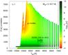 |
Fig. 11 Similar to Fig. 10, but for the the 0.1917 M⊙ sequence and the ELMV star SDSS J1614+1912. |
| In the text | |
|
Fig. 12 Similar to Fig. 10, but for the the 0.2019 M⊙ and 0.2389 M⊙ sequences and the ELMV stars SDSS J1518+0658 and SDSS J1618+3854. |
| In the text | |
|
Fig. 13 Similar to Fig. 10, but for the the 0.1762 M⊙ and 0.1805 M⊙ sequences and the ELMV stars SDSS J1112+1117, SDSS J1840+6423, and PSR J1738+0333. |
| In the text | |
|
Fig. 14 Periods of unstable ℓ = 1 modes in terms of the effective temperature, corresponding to the 0.1650 M⊙ and 0.1706 M⊙ sequences. Also shown are the pulsation periods of the ELMV star SDSS J1112+1117. The Teff adopted for the star is its 1D value corrected by 3D model atmosphere effects (see Table 2). |
| In the text | |
|
Fig. 15 Similar to Fig. 14, but for the case of PSR J1738+0333 and SDSS J1614+1912, and for the 0.1706 M⊙ and 0.1762 M⊙ sequences. |
| In the text | |
|
Fig. 16 Similar to Fig. 14, but for the case of SDSS J1618+3854 and for the 0.1762 M⊙ and 0.1805 M⊙ sequences. |
| In the text | |
|
Fig. 17 Similar to Fig. 14, but for the case of SDSS J1518+0658, and the 0.1917 M⊙ and 0.2019 M⊙ sequences. |
| In the text | |
Current usage metrics show cumulative count of Article Views (full-text article views including HTML views, PDF and ePub downloads, according to the available data) and Abstracts Views on Vision4Press platform.
Data correspond to usage on the plateform after 2015. The current usage metrics is available 48-96 hours after online publication and is updated daily on week days.
Initial download of the metrics may take a while.