| Issue |
A&A
Volume 585, January 2016
|
|
|---|---|---|
| Article Number | A31 | |
| Number of page(s) | 10 | |
| Section | Interstellar and circumstellar matter | |
| DOI | https://doi.org/10.1051/0004-6361/201527112 | |
| Published online | 10 December 2015 | |
The dark cloud TGU H994 P1 (LDN 1399, LDN 1400, and LDN 1402): Interstellar extinction and distance⋆
1 Institute of Theoretical Physics and Astronomy, Vilnius University, Goštauto 12, 01108 Vilnius, Lithuania
e-mail: This email address is being protected from spambots. You need JavaScript enabled to view it.
2 Vatican Observatory Research Group, Steward Observatory, Tucson, AZ 85721, USA
3 INAF Astronomical Observatory of Padova, 36012, Asiago (VI), Italy
Received: 4 August 2015
Accepted: 5 October 2015
Abstract
The results of CCD photometry in the seven-colour Vilnius system, for about 1000 stars down to V = 20 mag and their two-dimensional spectral types, are used to investigate the interstellar extinction in a 1.5 square degree area in the direction of the dark cloud TGU H994 P1 (LDN 1399, LDN 1400 and LDN 1402) in Camelopardalis. Photometric classification of 18 brightest stars down to V = 12 mag was verified by the spectra obtained with the 1.22 m telescope of the Asiago Observatory. The interstellar extinction run with distance is investigated with the results of photometry in the Vilnius system, and 504 red clump giants, identified by combining the results of infrared photometry from the 2MASS and WISE surveys. A possible distance of 140 ± 11 pc to the TGU H994 P1 cloud seems to be acceptable. Alternative distances of the cloud are discussed. The complex of the Camelopardalis clouds probably has a considerable depth along the line of sight, similar to that observed in the Taurus-Auriga complex. The maximum extinction AV in the dark filaments is found to be about 6.5 mag.
Key words: stars: fundamental parameters / ISM: clouds / ISM: individual: TGU H994 P1, LDN 1399, LDN 1400, LDN 1402
Full Table 2 is only available at the CDS via anonymous ftp to cdsarc.u-strasbg.fr (130.79.128.5) or via http://cdsarc.u-strasbg.fr/viz-bin/qcat?J/A+A/585/A31
© ESO, 2015
1. Introduction
A few years ago Straižys & Laugalys (2007, 2008) described a ring-like concentration of dust clouds located at the border of the Perseus, Camelopardalis, and Auriga constellations, which is perfectly seen in the Dobashi et al. (2005) atlas of dark clouds. The ring has a diameter of ~8° and is centred on the open cluster NGC 1528. Trying to test physical reality of this dust ring, we decided to investigate distances to its clouds and their extinction properties. The method of investigation is based on photometry of stars in the Vilnius seven-colour system, determination of their spectral and luminosity classes, reddenings, extinctions and distances. The first three catalogues of photometric data and spectral classification in the clouds TGU H1000, TGU H942, and TGU H994 were published by Zdanavičius et al. (2010) and Čepas et al. (2013a,b). In this paper, we present the investigation of interstellar reddening in the clump P1 of the TGU H994 cloud located in the northern side of the ring.
A curved ~5°-long chain of dark clouds, located westwards from the triple star 1 Cam (DL Cam, HD 28446), was described in the Barnard (1927) catalogue and atlas of dark clouds (clouds B8, B9, B11, B12). Barnard writes that this chain of dark clouds breaks up into more or less separate spots, “somewhat resembling those at the east end of the great lane from Rho Ophiuchi”. Again, dust clumps of this chain appear in the catalogues of dark clouds by Lynds (1962), Taylor et al. (1987), Dutra & Bica (2002), Dobashi et al. (2005), and Dobashi (2011). Unfortunately, it is not easy to cross-identify separate clouds in different catalogues since their boundaries usually remain indefinite. The present investigation covers the clump P1 of the cloud TGU H994 (Dobashi et al. 2005), which includes the Barnard cloud B11 and the Lynds clouds LDN 1399, LDN 1400, and LDN 1402.
Until now these clouds were investigated in the molecular bands: CO (Dickman 1975; Snell 1981; Myers & Benson 1983; Taylor et al. 1987; Dame et al. 1987, 2001; Park et al. 2004; Wu et al. 2012), H2CO (Dieter 1973; Minn & Greenberg 1973; Sandqvist et al. 1988; Clark 1991), NH3 (Myers & Benson 1983; Benson & Myers 1989; Clark 1991), CS, and N2H (Lee & Myers 1999). The local standard of rest (LSR) velocity of these clouds is 2–4 km s-1. Myers & Benson (1983) identified a group of visually opaque gas and dust condensations in the cloud LDN 1400 and the surrounding clouds, named cores, which are the supposed progenitors of young stars. Some of these objects are included in the catalogue of optically selected cores by Lee & Myers (1999). They were also observed with the Planck and Herschel satellites in the submillimeter and the far-infrared spectral regions (Juvela et al. 2012). About 30 far-infrared sources in the area of LDN 1400 and other nearby clouds were identified in the IRAS point-source catalogue by Clark (1991). Harjunpää et al. (1999) investigated polarization of stars in some directions of the LDN 1400 complex.
Distances to the chain clouds are known with a very low accuracy. The first estimate of their distance was probably published by Snell (1981). As the author explains, the estimate was done from the AV vs. d plot constructed for the stars with known B,V photometry and MK spectral types in a 20° × 20° region centred on the cloud. Although a value of d = 170 pc has been attributed to a small cloud in the group (LDN 1407, the size 8′ × 8′), actually this distance can be related to a much larger cloud complex. However, this distance should be of low accuracy since the stars with B,V photometry and MK spectral types in this region are rather scarce. This distance value (with nothing better available) has been used for decades in many investigations of the dust and molecular clouds in the whole chain. For the right group of the chain clouds (around LDN 1394), a distance value of 0.66 kpc was obtained by Juvela et al. (2012) applying a statistical method based on the Besancon stellar population synthesis model and the 2MASS photometry data1.
In several directions of the Camelopardalis dark clouds, the interstellar extinction was investigated by Zdanavičius et al. (1996, 2001, 2005), Zdanavičius & Zdanavičius (2002a,b, 2005) using seven-colour photometry in the Vilnius system and photometric classification of stars in spectral and luminosity classes. A common property of all areas is the extinction rise at 120–150 pc, reaching AV about 1.5–2.5 mag at 1 kpc. Thus, the Camelopardalis clouds are located almost at the same distance as the Taurus-Auriga star-forming region; see also the review article in the “Handbook of Star Forming Regions” by Straižys & Laugalys (2008).
Distances to dust clouds can be also estimated from interstellar line intensities observed in the spectra of foreground stars and the stars immersed in the cloud, usually of spectral classes B and A. The most detailed investigations of interstellar Na I D lines and Ca II H+K lines in the solar vicinity were published by Welsh et al. (1994, 2010), Sfeir et al. (1999), Vergely et al. (2001, 2010), Lallement et al. (2003, 2014), using the Hipparcos distances. In the general direction of Taurus and Auriga, the concentration of neutral gas is seen in the 80–150 pc distance range that can be associated with the boundary wall of the rarefied local cavity region around the Sun.
The TGU H994 P1 cloud is covered by one of the fields of the APOGEE2 spectral survey of red clump giants (RCGs, Bovy et al. 2014). From 155 RCGs in the field, 30 are located within our area, and the remaining are up to ~2° to the right and ~1.5° upwards from the investigated area. These stars are important tracers of the extinction at large distances, but they are lacking at the distances of cloud LDN 1400.
According to Dame et al. (1987, 2001), column densities and radial velocities of CO in some directions of the 2nd galactic quadrant exhibit two distinct layers at 800 pc and 300 pc from the Sun. The more distant layer, with the LSR velocity –12 km s-1, is related to the chain of OB associations at the outer edge of the Local Arm belonging to the Gould Belt. The closer layer with LSR velocity close to zero is related to the expanding gas ring discovered by Lindblad et al. (1973) from observations of neutral hydrogen; see also Lindblad (1974). In the direction of Cam-Per-Tau the Lindblad Ring can be also related to the Per OB3 (or α Per) association (d = 177 pc) and the Cas-Tau moving group of B-type stars (d from 125 to 300 pc); the distances are from de Zeeuw et al. (1999).
We found only four stars with the Hipparcos parallaxes in the investigated area: No. 13 = HIP 20327 (A0 V, d = 318 pc), No. 341 = HIP 20655 (A1 IV-V, d = 256 pc), No. 420 = HIP 20720 (B8 V, d = 3.5 kpc), and HD 28097 = HIP 20910 (F7 V, d = 81.5 pc, too bright for our CCD photometry). The star numbers are from the catalogue Čepas et al. (2013b), hereafter Paper I. The accuracy of parallaxes of the first three stars is rather low.
2. Photometric data and spectral types
Exposures of the area (Fig. 1) in the Vilnius seven-colour system were obtained in October of 2010 with the Maksutov-type 35/51 cm telescope of the Molėtai Observatory in Lithuania, equipped with a CCD camera. The area covers 1.5 deg2 with the centre at RA (J2000) = 04h25.5m, Dec (J2000) = +54°55′, ℓ = 150.53°, b = + 3.96°. More details about the observations and their processing are given in Paper I. The Vilnius photometric system UPXYZVS with the mean wavelengths 345, 374, 405, 466, 516, 544, and 656 nm is described in the Straižys (1992) monograph.
The catalogue published in Paper I gives the results of photometry for 727 stars down to V ≈ 17 mag. For about 73% of stars, two-dimensional spectral types (spectral and luminosity classes) were determined applying two classification codes based on interstellar reddening-free Q-parameters. One of these codes, COMPAR, applies a comparison of Q-parameters of stars in the area and individual standard stars (Straižys et al. 2013). The second code, now renamed to KLASQ, is described in Milašius et al. (2013). Instead of standard stars with known MK spectral types, it applies the intrinsic colour indices calibrated in MK types. In the present investigation, the stars of Paper I were reclassified anew with a modernized version of the second code (KLASQ), therefore, for some stars, new spectral and luminosity classes show small differences in comparison with Paper I.
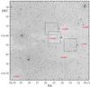 |
Fig. 1 Map with the observed area in the red filter (DSS1 Red from the SkyView Virtual Observatory). The three smaller squares were observed with the VATT telescope to fainter magnitudes. |
Additionally, for the classification of fainter stars down to V≈20 mag, we applied Vilnius photometry in three 12′ × 12′ areas located at the edges and within the LDN 1400 cloud. The areas are framed in Fig. 1 and their central coordinates are given in Table 1. We obtained CCD observations in the Vilnius system in November and December 2014 and January 2015 with the 1.8 m VATT telescope of the Vatican Observatory on Mt. Graham, Arizona. In each area we processed about 70 frames obtained with the exposures from 30 min to 5 s. Instrumental colour indices were transformed to the standard system with colour equations obtained from observations of the cluster M67 (Laugalys et al. 2004). The stars measured in Paper I served as zero-point standards of magnitudes and colour indices. The final adjustment of zero points has been done by optimizing the accuracy of photometric classification of a selected set of standard stars in the investigated area. We performed photometric classification of stars with the same COMPAR and KLASQ codes mentioned above, and the results were averaged.
The catalogue of photometric data for 855 stars down to V ≈ 20 mag and the results of photometric two-dimensional classification for about 65% of them will be accessible at the Strasbourg Data Center. Table 2 gives the beginning of this catalogue for the first ten stars. The columns list the following information: star number, equatorial coordinates J2000.0, magnitude V, colour indices U−V, P−V, X−V, Y−V, Z−V and V−S, and photometric spectral types in the MK system. Photometric spectral classes are given in lower-case letters to distinguish from spectroscopic classes. The suspected metal-deficient stars are designated as md:, and the metal-rich stars (Am) as mr:. The coordinates are from the PPMXL catalogue (Roeser et al. 2010) rounded to two decimals of time second and to one decimal of arcsecond.
The rms errors of the magnitudes V and colour indices X−V, Y−V, Z−V and V−S down to V = 16 mag are usually lower than 0.02 mag, and the errors of U−V and P−V are approximately twice as large. At V> 19 mag, the accuracy of photometry in the ultraviolet, especially for heavily reddened stars, is too low for reliable classification of stars earlier than K. For most of these stars the U−V and P−V colour indices are not given. Colour indices with σ = 0.05–0.10 mag are labelled with colons. The stars found to be binaries or having asymmetric images were not classified in luminosity classes, and in the column of spectral types these stars are designated with double asterisks.
The first ten stars of the data catalogue in the three VATT areas measured in the Vilnius seven-colour system.
To verify the results of photometric classification, one of us (U.M.) obtained the spectra of 18 stars of the area down to V = 12 mag with the 1.22 m telescope at the Asiago Observatory, Italy, equipped with a B&C spectrograph and a 600 lines/mm grating providing a dispersion of 1.17 Å/pix and a resolving power of FWHM (PSF) = 2.1 pix. The recorded spectra cover 3487–5885 Å. Spectral classification of these stars, listed in Table 3, was accomplished with the computer program MKCLASS designed to classify stellar spectra on the MK system provided by Gray & Corbally (2014). Table 3 shows that in most cases the differences between the spectroscopic and photometric spectral types do not exceed one to two spectral subclasses and one luminosity class. This gives us additional confidence in two-dimensional spectral types determined from Vilnius photometry.
As an independent check of the classification of the Asiago spectra by means of the Gray & Corbally (2014) code, we independently classified eight of them through a careful visual comparison of their calibrated spectra against the Yamashita et al. (1977) atlas of the representative stellar spectra in the MK system. For these stars (Nos. 8, 76, 279, 420, 565, 580, 668, and 683), differences between the spectral classification from photometry and from the Gray & Corbally (2014) code were the largest. The results, listed in Table 3, are in strong support of the MKCLASS code.
3. Interstellar extinctions and distances based on Vilnius photometry
For 584 stars from Paper I and for 447 stars from Table 2 with reliable spectral and luminosity classes, colour excesses EY−V, interstellar extinctions AV, and distances d (in pc) were calculated with the following equations: 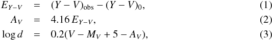 where V and Y−V are the observed magnitudes and colour indices. The intrinsic colour indices (Y−V)0 and absolute magnitudes MV for a given spectral type are from Straižys (1992). The errors of colour excesses, extinctions, and distances are described in Straižys et al. (2015), hereafter Paper II. Typical errors of the extinction and distance are σ(AV) /AV = ± 0.06, and σ(d) /d = ± 0.10.
In Eq. (2) the coefficient corresponds to the normal interstellar extinction law. The normality of the law was verified in the following way: (1) 123 B and A stars in the area were selected; (2) for these stars, EB−V = 1.32EY−V values were calculated; (3) the EV−J, EV−H, and EV−Ks values were calculated taking the intrinsic colours from Straižys (1992); (4) the RV values were calculated from the ratios EV−λ/EB−V with the equations from Fitzpatrick (1999), Fitzpatrick & Massa (2009) and Larson (2014). The resulting RV values are between 2.92 and 3.12, i.e. close to the normal value 3.1.
Stars classified from the Asiago spectra by the Gray & Corbally (2014) code MKCLASS and by visual inspection (U.M.).
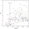 |
Fig. 2 Dependence of the extinction on distance for the investigated area up to d = 500 pc. The stars, measured in the Molėtai telescope exposures, are plotted as dots, and the stars, measured in the VATT exposures, are plotted as circles. Crosses are the stars for which MK spectral classes were determined from their Asiago spectra (Table 3). The nearest reddened stars are labelled with their numbers in the Paper I catalogue. The red vertical line designates the accepted position of the dust cloud TGU H994 P1 at 140 pc (see the text). The 3σ error bar for this distance is shown. |
The plot AV vs. d for stars in the whole 1.5 deg2 area up to 500 pc is shown in Fig. 2. The stars measured from the Molėtai telescope exposures are shown as dots, and those measured from the VATT exposures are shown as open circles. The stars with spectroscopic MK types (Table 3) are plotted as crosses. The red vertical line designates the accepted cloud distance as discussed in the next section.
The AV vs. d plot for 584 stars in the same area up to 5.5 kpc is shown in Fig. 3. The two broken curves show the limiting magnitude effect for stars of spectral types A0 V at V = 15 and 16 mag. Most stars are located below the last curve. Above it, at large distances, we find only a few stars of spectral class B and M giants, which have absolute magnitudes brighter than A0 V. Figure 4 shows the AV vs. d plot for 416 stars up to 5.5 kpc in the three areas observed with the VATT telescope down to fainter apparent magnitudes.
4. Distance to the TGU H994 P1 cloud
The determination of distances to dust clouds located close to the Sun is difficult because the number of stars in the foreground and immediately behind the cloud is usually low, and most of them are K and M dwarfs. The beginning of the cloud should be signified by a sudden rise of the extinction at a certain distance. However, the apparent distance of the nearest reddened stars cannot be accepted as the cloud distance, since their distances are affected by the errors of the observed magnitudes and colours, photometric classification errors, cosmic dispersion of the intrinsic colours, variations in the shape of the interstellar extinction law; some stars can be unresolved binaries.
In our case (Fig. 2), the distribution of stars with distance shows a significant increase of the extinction starting from ~110 pc. At about 200 pc the extinction values close to ~5 mag are being reached. Trying to understand where the cloud is located, we must analyse the possible distance errors for each of the scarce reddened stars. The largest source of distance errors are luminosity classes determined by photometric classification. In different ranges of spectral classes, these errors are somewhat different, but their typical value is close to 3σ = ± 0.5 mag. For K- and M-type dwarfs the photometric luminosity class is usually correct, but in the HR diagram they exhibit considerable intrinsic dispersion of their MV values at a fixed intrinsic colour or spectral class; see Perryman et al. (1995, 1997). An absolute magnitude error of ±0.5 mag leads to the minimum and maximum apparent distances 0.79 d and 1.26 d. As result of these distance errors, stars move from the distance of the cloud to both sides, but they are easy to identify in the direction of negative distance errors (i.e. reddened stars moved to foreground) since in the direction of positive distance errors they become mixed with reddened background stars (except at AV close to zero, see below).
At this point, we evaluate the distance to the cloud from the apparent positions of the reddened foreground stars. Since there is no information about their binarity, the stars are considered to be moved from the cloud distance mainly by the errors of their absolute magnitudes. Unfortunately, the close reddened stars in our sample are very scarce.
The reddened star with AV> 1 mag that is nearest to us is No. 428 (V = 13.47, k1 V, AV = 2.14 mag, d = 111 pc). This star is located only about 2′ north of the cloud LDN 1400 edge. If this star has been moved to this apparent distance by the 3σ error, its real distance should be 111 × 1.26 = 140 pc (all distances in this paragraph are rounded to 1 pc). If star No. 428 is a binary or has been shifted shortwards by a larger distance error, the calculated cloud distance should be larger. If the star has been moved by a smaller distance error, its real distance, i.e. beginning of the cloud, should be smaller.
Another place in the AV vs. d diagram is related to the unreddened or little reddened stars apparently located at larger distances than the cloud. If these stars have been moved to their apparent distances due to positive errors, then the real distance of the cloud should be smaller by a factor of 0.79. In Fig. 2, the stars with small extinction (AV< 0.2 mag) extend to the apparent distance 180 pc, and this allows us to estimate the real cloud distance at 180 × 0.79 = 142 pc. This value is in agreement with the distance given by the foreground star No. 428.
If these considerations are real, the cloud distance is at 140 pc with 3σ errors –31 pc and +36 pc shown by the error bar in Fig. 2. Within this box, ten reddened stars with AV between 0.5 and 2.3 mag are present. On the other hand, we are not sure that the entire investigated area is covered by a single cloud located at a fixed distance. The cloud complex can have considerable depth along the sightview, and in this case our results should correspond to different dust condensations. We return to this possibility in Sect. 6.
The star No. 396 (V = 10.15, G9 V, AV = 0.50, d = 62 pc), classified both from the Asiago spectra and from Vilnius photometry, also exhibits unusually large reddening for its distance. We suspect this may be caused by an unseen red dwarf companion.
Figures 3 and 4, which show the extinction vs. distance relations up to 5.5 kpc for the Molėtai and VATT telescopes, respectively, allow us to estimate the extinction run at large distances. The Molėtai results demonstrate a strong limiting magnitude effect at V = 16 mag. Therefore, the stars with large extinction values (up to ~3.7 mag) are only seen at distances closer than 2 kpc. In the VATT results, the limiting magnitude is close to V = 19 mag, and that is where we see the stars with AV up to 5 mag and at larger distances. Most of the heavily reddened stars are located close to the dark cloud LDN 1400 (VATT areas B and C). In Fig. 4, the absence of stars with AV lower than 2 mag can be explained by the fact that the VATT areas are located in directions with larger obscuration.
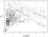 |
Fig. 3 Dependence of the extinction on distance for the investigated area up to 5.5 kpc for 584 stars with two-dimensional classification, measured in the Molėtai telescope exposures. The two broken curves show the limiting magnitude effect for A0 V at V = 15 and 16 mag. The exponential extinction formula of Parenago (1945) for the Galactic latitude b = 4°, AV = 1.25 mag/kpc and the scale height 100 pc is shown. |
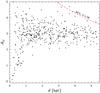 |
Fig. 4 Dependence of the extinction on distance in the three 12′ × 12′ areas for 416 stars with two-dimensional classification, measured in the VATT telescope exposures. The red broken curve designates the limiting magnitude effect for A0 V stars at V = 18 mag. |
5. The extinction based on 2MASS and WISE photometry of red clump giants
RCGs offer an additional possibility to investigate the interstellar extinction in the area. These stars have a low dispersion of their intrinsic colours and absolute magnitudes (Perryman et al. 1995, 1997; Alves 2000; Grocholski & Sarajedini 2002; Van Helshoecht & Groenewegen 2007; Groenewegen 2008), and this allows us to use them as standard candles. In this section, we briefly describe their photometric identification with the 2MASS J,H,Ks (Skrutskie et al. 2006) and the WISE W2 (Wright et al. 2010) near-infrared systems.
5.1. JHKs photometry
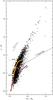 |
Fig. 5 J−H vs. H−Ks diagram for 3230 stars in investigated TGU H994 P1 area. Only stars with the magnitude errors ≤0.03 mag are plotted. The main sequence (MS, brown belt), the red giant branch (RGB, orange belt), the intrinsic locus of red clump giants (RCG, red circle), the intrinsic line of T Tauri stars (broken line) and the reddening line for AV = 2 mag are shown. |
Figure 5 shows the J−H vs. H−Ks diagram plotted for 3230 stars in the investigated TGU H994 P1 area (1.5 deg2) with the magnitude errors ≤0.03 mag. The intrinsic sequences of luminosity classes V and III, and the intrinsic position of RCGs are shown (Straižys & Lazauskaitė 2009). RCGs form a reddening belt which has the width H−Ks ≈ 0.1 mag and a slope of EJ−H/EH−Ks ≈ 2.0 (Straižys & Laugalys 2009). This belt covers the sequence of normal RGB stars of spectral classes G5 to M5 as well as unreddened or little reddened dwarfs of spectral classes K and M0–M3. Thus, the 2MASS system alone does not allow us to separate RCGs from other types of stars.
The equation of the reddening line of RCGs,  (4)was determined drawing it through the fixed intrinsic position of RCGs at J−H = 0.46, H−Ks = 0.09 and 24 stars on the RCG belt for which J−H> 1.5. At lower values of J−H, the reddening line is hidden within a crowding of stars of different temperatures, luminosities, and reddenings; see Fig. 5.
We also applied another, more reliable method to obtain the equation of the reddening line applying RCGs identified in the APOGEE high-resolution, near-infrared spectroscopic survey (Bovy et al. 2014). In the vicinity of the investigated area, we used 314 RCGs located in the four 3° diameter circular areas listed in Table 4. One of these APOGEE areas partly overlaps a part of our area. We only took the magnitudes with the errors ≤0.03 mag and without saturation. The J−H vs. H−Ks diagram for these RCGs is shown in Fig. 6. The equation of the reddening line, again drawn through the fixed intrinsic position of RCGs, is  (5)which is very close to that obtained for the reddened RCGs mixed with the core H-burning RGB stars; see Eq. (4).
Four APOGEE areas in the vicinity of the investigated area from which RCGs were taken to determine equations of interstellar reddening lines in different near-infrared two-colour diagrams.
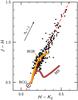 |
Fig. 6 J−H vs. H−Ks diagram for the 314 RCGs in four areas of the APOGEE survey listed in Table 4. Only the stars with the magnitude errors ≤0.03 mag are plotted. The designation of sequences and other symbols is the same as in Fig. 5. |
Next, we isolated 1667 stars that lie within the reddening belt of RCG and RGB stars limited by the following equations: 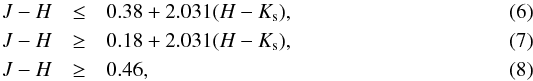 i.e. the belt width is Δ (H−Ks) = ± 0.10 mag, and it starts at the intrinsic position of RCGs (the circle in Fig. 5). In this belt, most RCGs should be present, but the J−H vs. H−Ks diagram is not sufficient for their identification. To make this possible, we need to deredden all RCG+RGB stars lying within this belt.
5.2. WISE photometry
For dereddening of RCG and RGB stars in Paper II, the H–[4.5] vs. J–[4.5] diagram has been used. Here [4.5] is the magnitude at 4.5 μm of the Spitzer IRAC system. This diagram was proposed by Majewski et al. (2011) for the determination of colour excesses and extinctions of F-G-K stars since the intrinsic colour indices H–[4.5] for most of them are close to zero. Since the Spitzer measurements in our area are absent, we changed [4.5] to the magnitude W2 of the WISE system with the mean wavelength at 4.6 μm (Wright et al. 2010; Jarrett et al. 2011). To decrease contamination of the sample by dwarfs, we rejected the stars with J−H< 0.46, the intrinsic colour of RCGs. The H−W2 vs. J−W2 diagram for 1320 stars, located in the J−H vs. H−Ks diagram within the RCG+RGB reddening belt, is shown in Fig. 7. The W2 magnitudes are taken from the All-WISE Data Release (Cutri et al. 2012), and their errors are limited to ±0.03 mag, as was the case with the magnitudes J, H, and Ks.
For the determination of the equation of the reddening line of RCGs in the diagram H−W2 vs. J−W2, we applied the same set of RCGs from four nearby areas of the APOGEE survey, as in the case of Fig. 6. Figure 8 shows that RCGs form a quite tight reddening line with a slope close to EH−W2/EJ−W2 = 0.51. The intrinsic point of RCGs in this diagram was determined applying two old open clusters, M67 and NGC 2506, which contain compact concentrations of RCGs and have small reddening (EB−V = 0.06 and 0.05, respectively). We selected four RCGs in M67 and nine RCGs in NGC 2506, free of close neighbours and with the errors of all magnitudes ≤0.03 mag. These 13 RCGs after dereddening are plotted in Fig. 8 (the lower compact group of dots), where they define the intrinsic position of RCGs at H−W2 = 0.07 and J−W2 = 0.56. The equation of the reddening line drawn through the APOGEE RCGs and the fixed intrinsic position is:  (9)
(9)
5.3. Identification of RCGs
We isolated RCGs in the H−W2 vs. J−W2 diagram of the investigated area (Fig. 7) with the following equations:  i.e. the width of the belt Δ (H−W2) = 0.1 mag has been taken, which corresponds to the scatter of the APOGEE RCGs (Fig. 8).
This list of RCGs, however, includes a considerable amount of unreddened and reddened dwarfs of spectral classes G–K–M, and subgiants of spectral classes G–K. For their elimination, we applied the magnitude-colour diagram Ks vs. H−Ks. In this diagram, late-type stars of luminosities V and IV form a clump of stars at the lower left corner with the vertical extension upwards along the H−Ks = 0.1 line; see Fig. 5 in Paper II. These stars were eliminated with the equations  (12)and
  (13)After application of the described procedures, the resulting list contains 837 suspected RCG stars. Undoubtedly, this list is contaminated by a certain amount of normal G–K giants and subgiants of RGB as well as K–M dwarfs. The percentage of this contamination and its possible consequences are estimated in the next section.
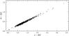 |
Fig. 7 H−W2 vs. J−W2 diagram for the investigated H994 P1 area. The stars from the RCG+RGB belt in the J−H vs. H−Ks diagram with the 2MASS and WISE magnitude errors ≤0.03 mag are plotted. |
 |
Fig. 8 H−W2 vs. J−W2 diagram for the 314 RCGs in four areas of the APOGEE survey listed in Table 4. We plot only the stars with the magnitude errors ≤0.03 mag. The group of 13 dots at H−W2 = 0.07, J−W2 = 0.56 are dereddened RCGs of clusters M67 and NGC 2506, defining the intrinsic position of RCGs. |
Colour excesses of the selected RCGs were determined as 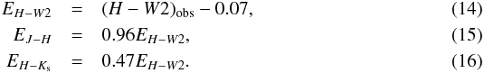 The last two equations were derived from the corresponding ratios for the Spitzer [4.5] mag (Paper II), and the equation
 ![Mathematical equation: \begin{eqnarray} E_{H-W2} = 1.035 E_{H-[4.5]}, \end{eqnarray}](/articles/aa/full_html/2016/01/aa27112-15/aa27112-15-eq111.png) (17)which we derived from the normal interstellar extinction law presented by McClure (2009).
(17)which we derived from the normal interstellar extinction law presented by McClure (2009).
In Fig. 9 dereddened RCGs are plotted in the (J−H)0 vs. (H−Ks)0 diagram. For control, in Fig. 10 we plot the same diagram for 314 APOGEE RCGs from the four areas listed in Table 4 and 13 RCGs from open clusters M67 and NGC 2506, all dereddened with the same method. In both figures, RCGs cover very similar areas. In Fig. 9 the RCG area has a form of a parallelogram with the sides defined by the RCG belts: the right and left sides are limited by Eqs. (6) and (7), and the lower and upper sides by (J−H)0 = 0.40 and 0.60, which follow from Eqs. (10), (11), (14), and (15). In both figures the centre of the largest concentration of RCGs corresponds to (J−H)0 = 0.48 and (H−Ks)0 = 0.10. Below we accept these values as intrinsic colours of RCGs. They are larger than the intrinsic colours of RCGs estimated by Straižys & Lazauskaitė (2009) just by 0.02 and 0.01 mag.
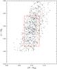 |
Fig. 9 Intrinsic (J−H)0 vs. (H−Ks)0 diagram for 837 stars in the investigated TGU H994 P1 area, the majority of which should be RCGs. Only the stars located inside the red rectangle were selected to investigate the extinction. |
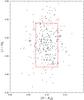 |
Fig. 10 Intrinsic (J−H)0 vs. (H−Ks)0 diagram for 314 dereddened RCGs from the four APOGEE areas (Table 4, dots) and from the open clusters M67 and NGC 2506 (circles). The red rectangle is duplicated from Fig. 9. |
Trying to decrease the contamination, we excluded all stars lying outside the rectangle centred on the intrinsic position of RCGs with side lengths of 0.12 mag in J−H and 0.06 mag in H−Ks. Within this rectangle 504 stars remain.
5.4. Interstellar extinction of RCGs
Interstellar extinctions and distances of the selected RCGs were determined with the following equations: ![Mathematical equation: \begin{eqnarray} A_{K_{\rm s}} &=& 0.67\,E_{J-K_{\rm s}} = 0.67\,\left[(J-K_{\rm s})_{\rm obs} - (J-K_{\rm s})_0\right], \\ \log d &=& 0.2\,\left(K_{\rm s} - M_{K_{\rm s}} +5 - A_{K_{\rm s}}\right), \end{eqnarray}](/articles/aa/full_html/2016/01/aa27112-15/aa27112-15-eq117.png) where (J−Ks)0 = 0.58 and MKs = –1.6 mag. The relative errors of the extinction and distance are σ(AKs) = ± 0.115 AKs and σ(d) /d = ± 0.042 (Paper II).
where (J−Ks)0 = 0.58 and MKs = –1.6 mag. The relative errors of the extinction and distance are σ(AKs) = ± 0.115 AKs and σ(d) /d = ± 0.042 (Paper II).
Figure 11 shows the AKs vs. d plot for the selected RCGs in the investigated area. The right y-axis shows the extinctions transformed to the AV scale with the equation 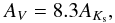 (20)which is valid for the normal interstellar extinction law.
 |
Fig. 11 Extinction AKs vs. distance in the investigated area for the RCGs identified combining the 2MASS and WISE magnitudes. The vertical line designates the accepted position of the cloud TGU H994 P1 at 140 pc. The red broken curve designates RCGs at the limiting magnitude Ks = 12.5 mag. |
6. Discussion
The distance to the cloud TGU H994 P1 estimated in Sect. 4 is based on the assumption that the reddened star No. 428 (k1 V) has appeared at 111 pc owing to a negative 3σ distance error. Then the true distance of this star should be at 140 pc, where the cloud causing its reddening is located. This result is also supported by a few stars with low extinction and distances up to 180 pc. If these stars are located in front of the cloud, i.e. at 140 pc, they could be shifted to their apparent positions because of positive 3σ distance errors. A distance of 140 pc is in agreement with the distance to the complex of the Taurus dark clouds located on the opposite side of the Milky Way (see references in Introduction). On the other hand, the Camelopardalis complex of dark clouds can be very deep along the sightline, as is the case with the Taurus complex, which has a depth of up to 50 pc or more, determined from radio interferometry of young stellar objects (Loinard et al. 2011) and from interstellar line strengths (Welsh et al. 2010; Lallement et al. 2014) combined with the Hipparcos parallaxes.
The investigated area is located at b = ~ 4°, and this means that with increasing distance our sightline recedes from the Galactic plane: the height above the plane is 70 pc at 1 kpc, 140 pc at 2 kpc, 280 pc at 4 kpc, etc. The expected extinction rise due to the diffuse dust layer near the plane (the Parenago law, Fig. 3) at d> 1 kpc should be rather low. Therefore, the extinction level at large distances must be defined mainly by the cloud with an additional small component caused by the diffuse dust layer. This is confirmed by the extinction versus distance plot in Fig. 4, where the results of deep classification of stars up to ~19 mag are shown. The minimum extinction in the most transparent directions remains at about 1.5–2 mag, and the maximum extinction in the directions where our sightline crosses peripheries of the dense clouds is between 4 and 5 mag. At the distances of the Perseus Arm and the Outer Arm, our sightline is about 100–140 pc and 350 pc above the plain. Thus, the influence of dust content in these two arms is not detectable.
Figure 11 shows that RCGs exhibit more or less the same minimum extinction level close to AV = 1.5–2 found for the other stars classified in the Vilnius system (Figs. 3 and 4). However, the maximum extinction is larger by about 1.5–2.5 mag, reaching about 6.5 mag in the dark filaments and around them.
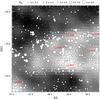 |
Fig. 12 Surface distribution of the extinction for RCGs. The five sizes of the circles correspond to different ranges of extinction. The five Lynds clouds are identified. The dust map from Schlegel et al. (1998) is shown in the background. |
In Fig. 12 we plot a map of RCGs identified in the investigated area with different sizes of circles for different ranges of the extinction. The smallest circles are for AKs between 0.1 and 0.3 mag, and the largest circles for AKs higher than 0.6 mag. In the background the dust map from Schlegel et al. (1998) based on the IRAS and COBE/DIRBE 100 μm emission observations is shown. It is evident that the largest circles concentrate on the darkest dust filaments, especially at LDN 1399, LDN 1400, and LDN 1402. The calibration of the dust maps by Schlafly & Finkbeiner (2011) in these clouds gives the values of AV between 4.5 and 4.9 mag3 in a good agreement with the values given by RCGs.
It is important to estimate the contamination of the identified RCG sample by stars of other types. Probably, most late-type dwarfs have been excluded by the constraints applied to the J−H vs. H−Ks, Ks vs. H−Ks, and H−W2 vs. J−W2 diagrams. However, the final list of RCGs can be contaminated by some amount of G8–K0 hydrogen-burning giants and subgiants of RGB. In our Paper II, we estimated about 50% contamination. In the present investigation the contamination percent must be smaller since for the calibration of the method we applied a large sample of true RCG stars selected with the physical parameters of stars determined from high-dispersion spectra. Since the reddened APOGEE RCGs were taken from nearby areas, the slopes of the interstellar reddening lines in two-colour diagrams should be free of the Galactic longitude effect.
The list of selected RCGs contained 46 stars classified with Molėtai photometry and 26 stars classified with VATT photometry. Among the Molėtai stars, 13 have been classified as dwarfs or subgiants, and this constitutes 28% of common stars. Among the VATT stars, the contamination by dwarfs and subgiants is about 20%. These wrong RCGs exhibit low values of the extinction at large distances; they were all excluded from the AKs vs. d plot (Fig. 11). We have no possibility to estimate the percentage of contamination by RGB G8–K0 giants. Fortunately, both RCGs and RGB giants of the same spectral classes have similar intrinsic colours (J−K)0 and absolute magnitudes MKs (see Paper II). Thus, their positions in the AKs vs. d plot should be not very different.
The clouds in the investigated area do not show active star formation. Radio observations in molecular lines reveal a number of cool gas cores of the subparsec sizes, which might be prestellar clumps. However, stellar YSOs in the area are quite scarce. In Fig. 5, only a few stars are located in the region of possible T Tauri stars. Among them, the most reliable candidate is 2MASS J04251408+5456524 at J−H = 1.53 and H−Ks = 0.97. Two more possible YSOs, 2MASS J04241953+5453594 and J04262976+5450399, are revealed by the Ks−W1 vs. W1−W2 diagram. These three stars all are seen in the direction of LDN 1400. A few stars located in Fig. 5 above the intrinsic T Tauri line (from Meyer et al. 1997) with J−H = 0.8–1.1 and H−Ks = 0.4–0.6 are candidates to be YSOs of class III (WTTS). These stars cannot be normal M dwarfs reddened by interstellar dust since in this case their distances calculated with Eq. (19) are unrealistically small (50–80 pc). Part of them can be binaries whose reddening is caused by a cooler secondary component.
7. Conclusions
We present the results of seven-colour photometry of 855 stars in the Vilnius photometric system down to V ≈ 20 mag in the vicinity of the dark cloud TGU H994 P1 (Dobashi et al. 2005). For about 65% of these stars, we determine their spectral and luminosity classes, colour excesses, extinctions AV, and distances. The new data supplement the catalogue of 727 stars in a larger area down to V ≈ 17 mag published earlier (Čepas et al. 2013b). For control, MK types of the 18 brightest stars were determined from the spectrograms obtained at the Asiago Observatory. In addition, we develop a method to identify red clump giants, applying infrared photometry from 2MASS and WISE surveys. The method is calibrated with the use of four areas of the high-dispersion spectral APOGEE survey, located in the vicinity of the investigated area. We used this method to identify 504 RCGs in the area down to Ks = 12.5 mag.
The results of photometric classification of about 1000 stars are applied to investigate the interstellar extinction in the area, covering about 1.5 deg2 and to estimate the distance to the dust cloud. At the distances >1 kpc, this investigation is supported by the extinctions of 504 RCGs. We found the distance to the cloud TGU H994 P1, based on a few stars, classified by the Vilnius colour indices and spectroscopically, to be close to 140 ± 11 pc. This result coincides with a distance of the Taurus dark clouds located on the opposite side of the Galactic equator. Alternative distances are also discussed. We do not exclude that the cloud complex in the investigated area has a considerable depth, such as the star-forming region in Taurus. Verification of distances to the reddened TGU H994 P1 stars will be soon possible with Gaia parallaxes.
The minimum extinction in the area of the order of 1.0–1.5 mag is well defined by the exponential Parenago law with AV = 1.25 mag/kpc. We observe maximum AV extinction up to about 6.5 mag in the dark cloud filaments and their vicinities. At distances >1 kpc, the mean extinction does not increase up to 5.5 kpc. This result is expected since our sightline crosses the Galaxy at 100–140 pc above the Perseus Arm and at ~350 pc above the Outer Arm.
In Table 1 of Juvela et al. (2012), the identification of the cloud LDN 1400 is not correct. It is located in the same area, called G150.47+3.93, as the LDN 1399 cloud.
Apache Point Observatory Galactic Evolution Experiment.
The NASA/IPAC Extragalactic Database, NED.
Acknowledgments
The use of the Simbad and SkyView databases is acknowledged. The project is partly supported by the Research Council of Lithuania, grant No. MIP-061/2013.
References
- Alves, D. R. 2000, ApJ, 539, 732 [NASA ADS] [CrossRef] [MathSciNet] [Google Scholar]
- Barnard, E. E. 1927, Vizier Online Data Catalogue: VII/220A [Google Scholar]
- Benson, P. J., & Myers, P. C. 1989, ApJS, 71, 89 [NASA ADS] [CrossRef] [Google Scholar]
- Bovy, J., Nidever, D. L., Rix, H. W., et al. 2014, ApJ, 790, 127 [NASA ADS] [CrossRef] [Google Scholar]
- Čepas, V., Zdanavičius, J., Zdanavičius, K., Straižys, V., & Laugalys, V. 2013a, Baltic Astron., 22, 223 [Google Scholar]
- Čepas, V., Zdanavičius, J., Zdanavičius, K., Straižys, V., & Laugalys, V. 2013b, Baltic Astron., 22, 243, Paper I [NASA ADS] [Google Scholar]
- Chojnowski, S. D., Whelan, D. G., & Wisniewski, J. P. 2015, AJ, 149, 7 [NASA ADS] [CrossRef] [Google Scholar]
- Clark, F. O. 1991, ApJS, 75, 611 [NASA ADS] [CrossRef] [Google Scholar]
- Cutri, R. M. et al. 2012, VizieR Online Data Catalog: II/311 [Google Scholar]
- Dame, T. M., Ungerechts, H., Cohen, R. S., et al. 1987, ApJ, 322, 706 [NASA ADS] [CrossRef] [Google Scholar]
- Dame, T. M., Hartmann, D., & Thaddeus, P. 2001, ApJ, 547, 792 [NASA ADS] [CrossRef] [Google Scholar]
- de Zeeuw, P. T., Hoogerwerf, R., de Bruijne, J. H. J., Brown, A. G. A., & Blaauw, A. 1999, AJ, 117, 354 [NASA ADS] [CrossRef] [Google Scholar]
- Dickman, R. L. 1975, ApJ, 202, 50 [NASA ADS] [CrossRef] [Google Scholar]
- Dieter, N. H. 1973, ApJ, 183, 449 [NASA ADS] [CrossRef] [Google Scholar]
- Dobashi, K. 2011, PASJ, 63, S1 [NASA ADS] [CrossRef] [Google Scholar]
- Dobashi, K., Uehara, H., Kandori, R., et al. 2005, PASJ, 57, S1 [NASA ADS] [CrossRef] [Google Scholar]
- Dutra, C. M., & Bica, E. 2002, A&A, 383, 631 [NASA ADS] [CrossRef] [EDP Sciences] [Google Scholar]
- Fitzpatrick, E. L. 1999, PASP, 111, 63 [NASA ADS] [CrossRef] [Google Scholar]
- Fitzpatrick, E. L., & Massa, D. 2009, ApJ, 699, 1209 [NASA ADS] [CrossRef] [Google Scholar]
- Gray, R. O., & Corbally, C. J. 2014, AJ, 147, 80 [NASA ADS] [CrossRef] [Google Scholar]
- Grocholski, A. J., & Sarajedini, A. 2002, AJ, 123, 1603 [NASA ADS] [CrossRef] [Google Scholar]
- Groenewegen, M. A. T. 2008, A&A, 488, 935 [NASA ADS] [CrossRef] [EDP Sciences] [Google Scholar]
- Harjunpää, P., Kaas, A. A., Carlqvist, P., & Gahm, G. F. 1999, A&A, 349, 912 [NASA ADS] [Google Scholar]
- Jarrett, T. H., Cohen, M., Masci, F., et al. 2011, ApJ, 735, 112 [NASA ADS] [CrossRef] [Google Scholar]
- Juvela, M., Ristorcelli, I., Pagani, L., et al. 2012, A&A, 541, A12 [NASA ADS] [CrossRef] [EDP Sciences] [Google Scholar]
- Lallement, R., Welsh, B. Y., Vergely, J.-L., et al. 2003, A&A, 411, 447 [EDP Sciences] [Google Scholar]
- Lallement, R., Vergely, J.-L., Valette, B., et al. 2014, A&A, 561, A91 [NASA ADS] [CrossRef] [EDP Sciences] [Google Scholar]
- Larson, K. A. 2014, PASP, 126, 27 [NASA ADS] [CrossRef] [Google Scholar]
- Laugalys, V., Kazlauskas, A., Boyle, R. P., et al. 2004, Baltic Astron., 13, 1 [NASA ADS] [Google Scholar]
- Lee, C. W., & Myers, P. C. 1999, ApJS, 123, 233 [NASA ADS] [CrossRef] [Google Scholar]
- Lindblad, P. O. 1974, in Kinematics and Ages of Stars Near the Sun, ed. L. Perek, 381 [Google Scholar]
- Lindblad, P. O., Grape, K., Sandqvist, A., & Schober, J. 1973, A&A, 24, 309 [NASA ADS] [Google Scholar]
- Loinard, L., Mioduszewski, A. J., Torres, R. M., et al. 2011, in Rev. Mex. Astron. Astrofis. Conf. Ser., 40, 205 [Google Scholar]
- Lynds, B. T. 1962, ApJS, 7, 1 [NASA ADS] [CrossRef] [Google Scholar]
- Majewski, S. R., Zasowski, G., & Nidever, D. L. 2011, ApJ, 739, 25 [NASA ADS] [CrossRef] [MathSciNet] [Google Scholar]
- McClure, M. 2009, ApJ, 693, L81 [NASA ADS] [CrossRef] [Google Scholar]
- Meyer, M. R., Calvert, N., & Hillenbrand, L. A. 1997, AJ, 114, 288 [NASA ADS] [CrossRef] [Google Scholar]
- Milašius, K., Boyle, R. P., Vrba, F. J., et al. 2013, Baltic Astron., 22, 181 [NASA ADS] [Google Scholar]
- Minn, Y. K., & Greenberg, J. M. 1973, A&A, 22, 13 [NASA ADS] [Google Scholar]
- Myers, P. C., & Benson, P. J. 1983, ApJ, 266, 309 [NASA ADS] [CrossRef] [Google Scholar]
- Parenago, P. P. 1945, AZh, 22, 129 [Google Scholar]
- Park, Y., Lee, C. W., & Myers, P. C. 2004, ApJS, 152, 81 [NASA ADS] [CrossRef] [Google Scholar]
- Perryman, M. A. C., Lindegren, L., Kovalevsky, J., et al. 1995, A&A, 304, 69 [NASA ADS] [Google Scholar]
- Perryman, M. A. C., Lindegren, L., Kovalevsky, J., et al. 1997, A&A, 323, L49 [NASA ADS] [Google Scholar]
- Roeser, S., Demleitner, M., & Schilbach, E. 2010, AJ, 139, 2440 [NASA ADS] [CrossRef] [Google Scholar]
- Sandqvist, A., Tomboulides, H., & Lindblad, P. O. 1988, A&A, 205, 225 [NASA ADS] [Google Scholar]
- Schlafly, E. F., & Finkbeiner, D. 2011, ApJ, 737, 103 [NASA ADS] [CrossRef] [Google Scholar]
- Schlegel, D. J., Finkbeiner, D. P., & Davis, M. 1998, ApJ, 500, 525 [NASA ADS] [CrossRef] [Google Scholar]
- Sfeir, D. M., Lallement, R., Crifo, F., & Welsh, B. Y. 1999, A&A, 346, 785 [NASA ADS] [Google Scholar]
- Skrutskie, M. F., Cutri, R. M., Stiening, R., et al. 2006, AJ, 131, 1163 [NASA ADS] [CrossRef] [Google Scholar]
- Snell, D. M. 1981, ApJS, 45, 121 [NASA ADS] [CrossRef] [Google Scholar]
- Straižys, V. 1992, Multicolor Stellar Photometry (Tucson, Arizona: Pachart Publishing House) http://www.itpa.lt/MulticolorStellarPhotometry/ [Google Scholar]
- Straižys, V., & Laugalys, V. 2007, Baltic Astron., 16, 167 [Google Scholar]
- Straižys, V., & Laugalys, V. 2008, in Handbook of Star Forming Regions 1, ed. B. Reipurth (ASP Monograph Publications), 294 [Google Scholar]
- Straižys, V., & Laugalys, V. 2009, Baltic Astron., 18, 141 [NASA ADS] [Google Scholar]
- Straižys, V., & Lazauskaitė, R. 2009, Baltic Astron., 18, 19 [Google Scholar]
- Straižys, V., Boyle, R. P., Janusz, R., et al. 2013, A&A, 554, A3 [NASA ADS] [CrossRef] [EDP Sciences] [Google Scholar]
- Straižys, V., Vrba, F. J., Boyle, R. P., et al. 2015, AJ, 149, 161, Paper II [NASA ADS] [CrossRef] [Google Scholar]
- Taylor, D. K., Dickman, R. L., & Scoville, N. Z. 1987, ApJ, 315, 104 [NASA ADS] [CrossRef] [Google Scholar]
- Van Helshoecht, V., & Groenewegen, M. A. T. 2007, A&A, 463, 559 [NASA ADS] [CrossRef] [EDP Sciences] [Google Scholar]
- Vergely, J.-L., Ferrero, R. F., Siebert, A., & Valette, B. 2001, A&A, 366, 1016 [NASA ADS] [CrossRef] [EDP Sciences] [Google Scholar]
- Vergely, J.-L., Valette, B., Lallement, R., & Raimond, S. 2010, A&A, 518, A31 [NASA ADS] [CrossRef] [EDP Sciences] [Google Scholar]
- Welsh, B. Y., Craig, N., Vedder, P. W., & Vallerga, J. V. 1994, ApJ, 437, 638 [NASA ADS] [CrossRef] [Google Scholar]
- Welsh, B. Y., Lallement, R., Vergely, J.-L., & Raimond, S. 2010, A&A, 510, A54 [NASA ADS] [CrossRef] [EDP Sciences] [Google Scholar]
- Wright, E. L., Eisenhardt, P. R. M., & Mainzer, A. K. 2010, AJ, 140, 1868 [NASA ADS] [CrossRef] [Google Scholar]
- Wu, Y., Liu, T., Meng, F., et al. 2012, ApJ, 756, 76 [NASA ADS] [CrossRef] [Google Scholar]
- Yamashita, Y., Nariai, K., & Norimoto, Y. 1977, An Atlas of Representative Stellar Spectra (University of Tokyo Press) [Google Scholar]
- Zdanavičius, J., & Zdanavičius, K. 2002a, Baltic Astron., 11, 75 [NASA ADS] [Google Scholar]
- Zdanavičius, J., & Zdanavičius, K. 2002b, Baltic Astron., 11, 441 [Google Scholar]
- Zdanavičius, J., & Zdanavičius, K. 2005, Baltic Astron., 14, 1 [NASA ADS] [Google Scholar]
- Zdanavičius, J., Zdanavičius, K., & Kazlauskas, A. 1996, Baltic Astron., 5, 563 [NASA ADS] [Google Scholar]
- Zdanavičius, J., Černis, K., Zdanavičius, K., & Straižys, V. 2001, Baltic Astron., 10, 349 [NASA ADS] [Google Scholar]
- Zdanavičius, J., Zdanavičius, K., & Straižys, V. 2005, Baltic Astron., 14, 31 [Google Scholar]
- Zdanavičius, J., Čepas, V., Zdanavičius, K., & Straižys, V. 2010, Baltic Astron., 19, 197 [NASA ADS] [Google Scholar]
All Tables
The first ten stars of the data catalogue in the three VATT areas measured in the Vilnius seven-colour system.
Stars classified from the Asiago spectra by the Gray & Corbally (2014) code MKCLASS and by visual inspection (U.M.).
Four APOGEE areas in the vicinity of the investigated area from which RCGs were taken to determine equations of interstellar reddening lines in different near-infrared two-colour diagrams.
All Figures
|
Fig. 1 Map with the observed area in the red filter (DSS1 Red from the SkyView Virtual Observatory). The three smaller squares were observed with the VATT telescope to fainter magnitudes. |
| In the text | |
|
Fig. 2 Dependence of the extinction on distance for the investigated area up to d = 500 pc. The stars, measured in the Molėtai telescope exposures, are plotted as dots, and the stars, measured in the VATT exposures, are plotted as circles. Crosses are the stars for which MK spectral classes were determined from their Asiago spectra (Table 3). The nearest reddened stars are labelled with their numbers in the Paper I catalogue. The red vertical line designates the accepted position of the dust cloud TGU H994 P1 at 140 pc (see the text). The 3σ error bar for this distance is shown. |
| In the text | |
|
Fig. 3 Dependence of the extinction on distance for the investigated area up to 5.5 kpc for 584 stars with two-dimensional classification, measured in the Molėtai telescope exposures. The two broken curves show the limiting magnitude effect for A0 V at V = 15 and 16 mag. The exponential extinction formula of Parenago (1945) for the Galactic latitude b = 4°, AV = 1.25 mag/kpc and the scale height 100 pc is shown. |
| In the text | |
|
Fig. 4 Dependence of the extinction on distance in the three 12′ × 12′ areas for 416 stars with two-dimensional classification, measured in the VATT telescope exposures. The red broken curve designates the limiting magnitude effect for A0 V stars at V = 18 mag. |
| In the text | |
|
Fig. 5 J−H vs. H−Ks diagram for 3230 stars in investigated TGU H994 P1 area. Only stars with the magnitude errors ≤0.03 mag are plotted. The main sequence (MS, brown belt), the red giant branch (RGB, orange belt), the intrinsic locus of red clump giants (RCG, red circle), the intrinsic line of T Tauri stars (broken line) and the reddening line for AV = 2 mag are shown. |
| In the text | |
|
Fig. 6 J−H vs. H−Ks diagram for the 314 RCGs in four areas of the APOGEE survey listed in Table 4. Only the stars with the magnitude errors ≤0.03 mag are plotted. The designation of sequences and other symbols is the same as in Fig. 5. |
| In the text | |
|
Fig. 7 H−W2 vs. J−W2 diagram for the investigated H994 P1 area. The stars from the RCG+RGB belt in the J−H vs. H−Ks diagram with the 2MASS and WISE magnitude errors ≤0.03 mag are plotted. |
| In the text | |
|
Fig. 8 H−W2 vs. J−W2 diagram for the 314 RCGs in four areas of the APOGEE survey listed in Table 4. We plot only the stars with the magnitude errors ≤0.03 mag. The group of 13 dots at H−W2 = 0.07, J−W2 = 0.56 are dereddened RCGs of clusters M67 and NGC 2506, defining the intrinsic position of RCGs. |
| In the text | |
|
Fig. 9 Intrinsic (J−H)0 vs. (H−Ks)0 diagram for 837 stars in the investigated TGU H994 P1 area, the majority of which should be RCGs. Only the stars located inside the red rectangle were selected to investigate the extinction. |
| In the text | |
|
Fig. 10 Intrinsic (J−H)0 vs. (H−Ks)0 diagram for 314 dereddened RCGs from the four APOGEE areas (Table 4, dots) and from the open clusters M67 and NGC 2506 (circles). The red rectangle is duplicated from Fig. 9. |
| In the text | |
|
Fig. 11 Extinction AKs vs. distance in the investigated area for the RCGs identified combining the 2MASS and WISE magnitudes. The vertical line designates the accepted position of the cloud TGU H994 P1 at 140 pc. The red broken curve designates RCGs at the limiting magnitude Ks = 12.5 mag. |
| In the text | |
|
Fig. 12 Surface distribution of the extinction for RCGs. The five sizes of the circles correspond to different ranges of extinction. The five Lynds clouds are identified. The dust map from Schlegel et al. (1998) is shown in the background. |
| In the text | |
Current usage metrics show cumulative count of Article Views (full-text article views including HTML views, PDF and ePub downloads, according to the available data) and Abstracts Views on Vision4Press platform.
Data correspond to usage on the plateform after 2015. The current usage metrics is available 48-96 hours after online publication and is updated daily on week days.
Initial download of the metrics may take a while.