| Issue |
A&A
Volume 585, January 2016
|
|
|---|---|---|
| Article Number | A74 | |
| Number of page(s) | 16 | |
| Section | Interstellar and circumstellar matter | |
| DOI | https://doi.org/10.1051/0004-6361/201525915 | |
| Published online | 22 December 2015 | |
Molecule survival in magnetized protostellar disk winds
II. Predicted H2O line profiles versus Herschel/HIFI observations
1
LERMA, Observatoire de Paris, PSL Research University, CNRS, UMR
8112,
75014
Paris,
France
e-mail:
This email address is being protected from spambots. You need JavaScript enabled to view it.
2
LESIA, Observatoire de Paris, PSL Research University,
CNRS, 92190
Meudon,
France
3
Sorbonne Universités, UPMC Univ. Paris 06, 75005
Paris,
France
4
IPAG, UMR 5521 du CNRS, Observatoire de Grenoble,
38041
Grenoble Cedex,
France
5
IAS, UMR 8617 du CNRS, Université de Paris-Sud,
91405
Orsay,
France
Received: 17 February 2015
Accepted: 15 September 2015
Abstract
Context. The origin of molecular protostellar jets and their role in extracting angular momentum from the accreting system are important open questions in star formation research. In the first paper of this series we showed that a dusty magneto-hydrodynamic (MHD) disk wind appeared promising to explain the pattern of H2 temperature and collimation in the youngest jets.
Aims. We wish to see whether the high-quality H2O emission profiles of low-mass protostars, observed for the first time by the HIFI spectrograph on board the Herschel satellite, remain consistent with the MHD disk wind hypothesis, and which constraints they would set on the underlying disk properties.
Methods. We present synthetic H2O line profiles predictions for a typical MHD disk wind solution with various values of disk accretion rate, stellar mass, extension of the launching area, and view angle. We compare them in terms of line shapes and intensities with the HIFI profiles observed by the WISH key program towards a sample of 29 low-mass Class 0 and Class 1 protostars.
Results. A dusty MHD disk wind launched from 0.2–0.6 AU AU to 3–25 AU can reproduce to a remarkable degree the observed shapes and intensities of the broad H2O component observed in low-mass protostars, both in the fundamental 557 GHz line and in more excited lines. Such a model also readily reproduces the observed correlation of 557 GHz line luminosity with envelope density, if the infall rate at 1000 AU is 1–3 times the disk accretion rate in the wind ejection region. It is also compatible with the typical disk size and bolometric luminosity in the observed targets. However, the narrower line profiles in Class 1 sources suggest that MHD disk winds in these sources, if present, would have to be slower and/or less water rich than in Class 0 sources.
Conclusions. MHD disk winds appear as a valid (though not unique) option to consider for the origin of the broad H2O component in low-mass protostars. ALMA appears ideally suited to further test this model by searching for resolved signatures of the warm and slow wide-angle molecular wind that would be predicted.
Key words: astrochemistry / line: profiles / magnetohydrodynamics (MHD) / stars: jets / stars: protostars / ISM: jets and outflows
© ESO, 2015
1. Introduction
Supersonic bipolar jets are ubiquitous in young accreting stars from the initial deeply embedded phase (called Class 0) – where most of the mass still lies in the infalling envelope – through the late infall phase (Class 1) – where most of the mass is in the central protostar – to optically revealed young stars (Class 2 or T Tauri phase) – where the envelope has dissipated, but residual accretion continues through the circumstellar disk. The similarities in jet collimation, variability timescales, and ejection efficiency among these three phases suggests that robust universal processes are at play. In particular, the high kinetic power estimated in these jets (at least 10% of the accretion luminosity in low-mass sources) and the evidence that they are collimated on very small scales ≤20–50 AU suggests that magneto-hydrodynamic (MHD) processes play a key role and that jets could remove a significant fraction of the gravitational energy and excess angular momentum from the accreting system (see e.g. Frank et al. 2014, for a recent review). However, it is still unclear which parts of the MHD jet arise from a stellar wind (Sauty & Tsinganos 1994; Matt & Pudritz 2008), the interaction zone between stellar magnetosphere and inner disk edge (Shu et al. 1994; Zanni & Ferreira 2013) and/or the Keplerian disk surface (hereafter D-wind, Blandford & Payne 1982; Konigl & Pudritz 2000). Global semi-analytical solutions, confirmed by numerical simulations, have shown that the presence and radial extent of steady magneto-centrifugal D-winds in young stars depend chiefly on the distribution of vertical magnetic fields and diffusivity in the disk (see e.g. Casse & Ferreira 2000; Sheikhnezami et al. 2012). Both of these quantities have a fundamental impact on the disk angular momentum extraction, turbulence level, and planet formation and migration (see reviews by Turner et al. 2014; Baruteau et al. 2014). Finding observational diagnostics that can establish or exclude the presence of MHD D-winds in young stars is thus essential not only to pinpoint the exact origin of protostellar jets, but also to better understand disk accretion and planet formation.
Possible signatures of jet rotation consistent with steady D-winds launched from 0.1–30 AU have been claimed in several atomic and molecular protostellar jets, using HST or millimeter interferometers (see e.g. Frank et al. 2014, for a recent review). However, the resolution currently achieved across the jet beam is not yet sufficient to fully disentangle other effects such as asymmetric shocks or jet precession/orbital motion. Another independent and powerful diagnostic of the possible presence and radial extent of an extended D-wind is the molecular richness and temperature of the flow. In the first paper of this series (Panoglou et al. 2012), we investigated the predicted thermo-chemical structure of a steady self-similar dusty D-wind around low-mass protostars of varying accretion rates, taking into account the wind irradiation by far-ultraviolet (FUV) and X-ray photons from the accretion shock and the stellar corona. We confirmed the pioneering insight of Safier (1993) that H2 molecules can survive beyond some critical launch radius rc ≃ 0.2–1 AU, and showed that the wind is heated up to T ≃ 500–2000 K by ambipolar ion-neutral friction with both rc and T increasing with decreasing wind density. The predicted evolutions of molecular jet temperature, collimation, and speed with evolutionary stage were found qualitatively consistent with existing observational trends. We also predicted a high abundance of H2O along dusty streamlines launched from 1 AU. This emerged as a natural consequence of the D-wind heating by ion-neutral drag, which allowed quick gas-phase reformation of H2O by endothermic reactions of O and OH with H2 to balance FUV photodissociation. This temperature-dependence of H2O abundance, combined with a more density-sensitive line excitation than for CO (due to a much larger dipole moment) means that H2O emission appears as a particularly promising discriminant diagnostic of extended dusty D-winds in young low-mass stars.
Thanks to the exquisite sensitivity of the HIFI spectrometer on board the Herschel satellite, high-quality line profiles of H2O emission were obtained for the first time towards a wide sample of low-mass protostars and their outflows. Off-source spectra are dominated by localized shocked regions created by time variable ejection and interaction with the ambient medium (see e.g. Lefloch et al. 2012; Santangelo et al. 2012). Hence their varied line shapes trace disturbed flow dynamics that do not reflect the initial wind structure. In contrast, on-source spectra encompass only the innermost ≃5000 AU (at the distance of Perseus), which may still carry the imprint of the initial wind structure established by the acceleration process. On-source H2O HIFI spectra were acquired towards 29 low-mass protostars, in the course of the WISH key program (van Dishoeck et al. 2011). They differ from off-source spectra in revealing the presence of three roughly Gaussian velocity components at the flow base, with common properties across the whole sample (Kristensen et al. 2012; Mottram et al. 2014): a narrow central component arising from the infalling envelope; a medium component, slightly offset to the blue and detected only in a few sources, interpreted as a dissociative compact “spot-shock” between a wide-angle wind and the swept-up outflow cavity (Kristensen et al. 2013); and a ubiquitous broad component (BC) centered near systemic velocity and extending up to ±50 km s-1, which usually dominates the total H2O flux and is still of unclear origin. Low-J CO line profiles in the same sources only start tracing the BC for J = 10 owing to a much stronger contribution in CO from the envelope and the cool swept-up outflow cavity (Yıldız et al. 2013). Hence, H2O profiles appear as the current best specific tracer for constraining the physical origin of the BC, and we concentrate on this tracer in the following. Average excitation conditions and emission sizes for the BC were recently estimated by (Mottram et al. 2014) based on a multi-line H2O analysis, and an origin in thin irradiated C-shocks along the outflow cavity walls was proposed. A full chemical-dynamical model of this situation with line profile predictions remains to be developed to test this hypothesis. An alternative worth considering is that the BC in H2O might trace dusty MHD D-winds heated by ambipolar diffusion (the same heating process as in magnetized C-shocks), since those winds are also naturally expected to be water-rich for the reasons noted above, and to cover a broad range of flow velocities (due to their broad range of launch radii). Testing this alternative scenario against BC observations is an important goal, as it may set strong constraints on ill-known fundamental properties of Keplerian disks in protostars such as their size, accretion rate, and magnetization, which are central elements for modern theories of disk formation and magnetic braking in star formation (see Li et al. 2014, for a recent review).
In the present paper, we thus go one step further in exploring observational diagnostics of steady, self-similar dusty MHD D-winds by presenting synthetic H2O line profiles and comparing them to HIFI/Herschel observations of young low-mass Class 0 and Class I sources. Our specific goals are to see (1) whether a typical MHD D-wind is able to reproduce the range of H2O line profile shapes and intensities of the BC – an excessive predicted flux could argue against the presence of extended molecular D-winds in these sources – and (2) which range of launch radii and disk accretion rates would be implied if a D-wind were indeed the dominant contributor to the H2O BC. Section 2 describes the model improvements made since Paper I and the parameter space explored. Section 3 presents the calculated temperature and water gas-phase abundance in our D-wind model, and the effect of various system parameters on the emergent H2O line profiles. Section 4 demonstrates the excellent agreement between our synthetic line predictions and HIFI on-source spectra of low-mass protostars in terms of line profile shapes, absolute and relative intensities, and correlation with envelope density. Section 5 verifies whether the D-wind model explored here for the origin of the BC would also be consistent with independent observational constraints on disk size, accretion luminosity, and inclination in low-mass protostars. Section 6 summarizes our main conclusions and future prospects.
2. Model description
2.1. Dynamics and thermo-chemistry
Our modeling work is based on the thermo-chemical model of dusty MHD disk winds developed in (Panoglou et al. 2012, hereafter Paper I), where all the model ingredients are presented in detail. We only give a brief summary of the main elements here, and present the improvements made in order to obtain line profile predictions in H2O comparable to Herschel/HIFI observations.
The wind dynamics are prescribed using a self-similar, steady, axisymmetric MHD solution of accreting-ejecting Keplerian disks computed by Casse & Ferreira (2000) with a prescribed heating function at the disk surface (known as “warm” disk wind solution). It assumes a thermal pressure scale-height h = 0.03r (where r denotes the cylindrical radius), and has a magnetic lever arm parameter λ ≃ (rA/r0)2 = 13.8, where rA is the (cylindrical) radius of the wind Alfvén point along the magnetic surface anchored at r0 in the disk midplane. This particular solution was chosen because (i) the small λ value gives a good match to the tentative rotation signatures reported at the base of the DG Tauri atomic jet (Pesenti et al. 2004) and of other T Tauri jets (Ferreira et al. 2006) and (ii) the higher wind mass-loading (ξ ≃ 1/(2λ − 2) ≃ 0.04) is more consistent with observed atomic jet mass-fluxes than vertically isothermal “cold” solutions with large λ values (Garcia et al. 2001a; Ferreira et al. 2006). The chosen solution provides the non-dimensional streamline shape and distribution of velocity, density, and Lorentz force along it as a function of polar angle θ. The 2D density distribution and streamlines for typical source parameters are illustrated in Fig. 1 of Paper I.
Because the dynamical timescales for crossing the inner few 1000 AU of the jet are short, tdyn ~ 100 yr × (r0/ AU)1.5, the gas temperature, ionization level, and chemical abundances in the disk wind are generally out of equilibrium. The time-dependent thermo-chemistry of the gas must therefore be integrated numerically along each streamline as a function of altitude z above the midplane. The code performing this calculation is based on the C-shock model of Flower & Pineau des Forêts (2003) with additional treatment for the effect of stellar coronal X-rays and of FUV photons from the accretion hot spots (attenuated by gas and dust on the inner streamlines of the disk wind). The various heating, cooling, and chemical processes along the dusty streamlines are described and discussed in detail in Paper I.
In order to obtain reliable predictions in H2O lines, the thermo-chemical model from Paper I was upgraded in several ways:
-
1.
self-consistent, non-local calculation of H2 and CO self-shielding (see Appendix A);
-
2.
time-dependent integration of NLTE rotational level populations of H2O and the corresponding gas heating/cooling (see Appendix B);
-
3.
calculation of dust temperature including the dust opacity to its own radiation (see Appendix C);
-
4.
refined initial chemical abundances at the base of streamlines (see Appendix D).
As in Paper I, we will assume that the atomic MHD disk wind starts at a typical inner disk truncation radius of 0.07 AU (where it starts to provide gas extinction against coronal X-rays), while the first calculated molecular streamline is launched from the dust sublimation radius, Rsub. The thermo-chemical evolution is then calculated for a series of streamlines with launch radii r0 ranging from Rsub to a freely specified maximum value  ≤ 25 AU. The thermo-chemical integration starts just above the disk surface at the wind slow point, located at z ≃ 1.7h ≃ 0.05r0, and stops at z ≃ 1000r0 (z/r ≃ 20) where streamlines start to bend inwards. A recollimation shock may form beyond this point, and the steady dynamical solution would no longer be valid.
The parameters describing the stellar radiation field remain as in Paper I, where the reader is referred for a justification of these assumptions: (1) a stellar photosphere of effective temperature T⋆ = 4000 K and radius R⋆ = 3 R⊙, producing a luminosity L⋆= 2.1 L⊙; (2) a hard thermal X-ray spectrum of characteristic energy kBTX = 4 KeV and luminosity LX = 1030 erg s-1, typical of active coronae in young low-mass stars; and (3) an accretion hot spot emitting as a blackbody of temperature Ths = 10 000 K and luminosity Lhs equal to half of the accretion luminosity Lacc = GM⋆Ṁacc/R⋆. The hot-spot luminosity is thus the only radiative contribution that will vary from model to model (see Table 1).
2.2. Model grid
Models in order of increasing source accretion age and decreasing wind density.
The 2D spatial distribution of density, velocity and electric current values in the disk wind is obtained from the non-dimensional MHD solution by prescribing two free dimensional parameters: the stellar mass, M⋆, and the accretion rate in the disk ejecting zone, Ṁacc. Each pair of values (M⋆,Ṁacc) defines a so-called “source model”. Because the stellar mass and disk accretion rate are still poorly known in most protostars, and each combination requires a large number of CPU-consuming thermo-chemical calculations, we only explored a restricted grid of four source models summarized in Table 1, meant to represent typical parameters for low-luminosity Class 0 and Class 1 sources:
-
two values of stellar mass: following Paper I, we adopt M⋆ = 0.1 M⊙ for our Class 0 models, and M⋆= 0.5 M⊙ for our Class 1 models (where the star has accreted most of its final mass);
-
two values of accretion rate for each stellar mass: for the Class 0 models we consider 5 × 10⁻⁶ M⊙ yr-1 (standard Class 0 from Paper I = S0 model) and 2 × 10⁻⁵ M⊙ yr-1 (extreme Class 0 = X0 model). For the Class 1 sources we consider 10-6 M⊙ yr-1 (standard Class 1 from Paper I = S1 model), and 5 × 10⁻⁶ M⊙ yr-1 (extreme Class 1 = X1 model).
The range of Ṁacc values in our Class 0 and Class 1 models is in line with the predictions of recent 3D resistive MHD simulations of collapsing low-mass protostars (see Fig. 7 in Machida & Hosokawa 2013). The corresponding characteristic accretion ages tacc = M⋆/Ṁacc are 0.5–2 × 10⁴ yr for the Class 0 models and 1–5 × 10⁵ yr for the Class 1 models.
We note that because the model is self-similar, the wind velocity field scales as M⋆0.5 (Keplerian law), while the wind density field scales as nH∝Ṁacc . The latter scaling is the same as for an envelope in free fall at rate Ṁacc onto a point mass M⋆. Therefore, we can characterize how dense each wind model is by using the density such a fiducial envelope would have at 1000 AU as a proxy. This parameter, which we denote as
  (1000 AU), is listed in Col. 4 of Table 1 and shows that the wind density drops by a factor ≃45 in total from model X0 to model S1. Table 1 also lists the hot-spot luminosity Lhs = 0.5Lacc for each source model, and the corresponding dust sublimation radius Rsub calculated as described in Appendix C.
For each source model, the synthetic emergent line profiles depend on two additional free parameters, namely the maximum radial extension of the emitting MHD disk wind, and the inclination angle i of the disk axis to the line of sight. For the present exploratory study, we restricted ourselves to the following coarse grid:
-
four values of
: 3.2, 6.4, 12.8 and 25 AU; -
three values of the inclination angle i : near pole-on (30°), median (60°) and near edge-on (80°).
By varying the four free parameters (M⋆,Ṁacc,, i) we thus obtain a grid of 2 × 2 × 4 × 3 = 48 synthetic line profiles for each H2O line and source distance d. Synthetic channel maps are computed using the same method as in Cabrit et al. (1999), Garcia et al. (2001a) for optical forbidden lines, except that the line emissivity at each (r,z,φ) is now multiplied by the escape probability in the observer’s direction to account for the large H2O line opacity and its anisotropy (see Appendix B ). Channel maps are then convolved by the Herschel beam at the line frequency for the specified source distance, and the flux towards the central source in each channel map is used to build the predicted line profile as a function of radial velocity.
3. Model results
3.1. Gas temperature
Figure 1 presents color maps of the calculated distribution of gas temperature in our four wind models. Two-dimensional interpolation was applied between the discrete calculated streamlines to fill the r,z plane. As shown by Safier (1993), Garcia et al. (2001b) and Paper I, the main heating term is ion-neutral drag (denoted Γdrag hereafter). This process arises because the neutral fluid cannot feel the Lorentz force that accelerates the MHD disk-wind directly, and thus lags behind the accelerated charged particles. This velocity drift generates ion-neutral collisions that drag along and accelerate the neutrals, but also degrade the kinetic energy of drift motions into heat. It is the very same process that dissipates kinetic energy and provides gas heating in C-type shocks. Hence there are definite analogies between the thermal (and chemical) structure of molecular MHD disk-winds and that of C-shocks, as noted in Paper I, except that the heating rate and spatial scale are set here by the dynamics of MHD wind acceleration instead of the velocity jump in C-shocks.
It can be seen in Fig. 1 that overall the wind gets warmer from right to left in this figure as Ṁacc drops and M⋆ increases. This stems from the way Γdrag scales with Ṁacc and M⋆ and adjusts to balance adiabatic and radiative cooling (see Paper I). Typical temperatures on intermediate streamlines are ≃100 K in the extreme Class 0, ≃300 K in the standard Class 0, ≃600 K in the extreme Class 1, and ≃1000 K in the standard Class 1. Within a given source model, the gas temperature decreases while r0 increases, again because of the scaling of Γdrag with r0 (see Paper I). The slightly higher dust temperature compared with Paper I, due to the inclusion of photon-trapping, only affects the gas temperature at the dense wind base where gas and dust are well coupled.
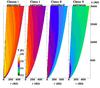 |
Fig. 1 Two-dimensional cuts of the calculated gas kinetic temperature (on a log10 scale) in the four source models with the parameters given in Table 1. The black contour levels are at 250, 400, 800, and 1600 K. The streamlines have launch radii ranging from the sublimation radius Rsub to 25 AU. The calculations were stopped inside the cone with z/r = 20 where streamlines start to recollimate towards the axis and shocks may later develop. The wind density drops from right to left successively by a factor 4, |

Chemical reactions affecting the H2O gas-phase abundance in our models.
3.2. Water gas-phase abundance
Our thermo-chemical model includes 1150 chemical reactions of various types (neutral-neutral and ion-neutral reactions, collisional dissociation, recombinations with electrons, charge exchange with atoms, molecules, grains and PAHs, photodissociation and photoionization by FUV and X-ray photons; see Paper I), out of which 104 involve gas-phase H2O. However, only three types of reactions are shorter than the wind dynamical timescale and thus play an actual role in the evolution of the wind H2O gas-phase abundance, namely: formation by endo-energetic neutral-neutral reaction of O and OH with H2 (dominant at the base of the wind), formation by dissociative recombination of H3O+ (dominant in the cooler outer wind regions), and photodissociation by FUV radiation emitted by the accretion shock on the stellar surface (attenuated by dust along intervening wind streamlines). The adopted rates for these significant reactions1 are listed in Table 2. Photodissociation by secondary FUV photons generated by the interaction of stellar X-rays and cosmic rays with molecular gas (Gredel et al. 1989) is also included in the model, but is too slow to have an effect. Since H2O ice mantles are fully thermally desorbed at the base of the wind for r0 ≤ 25 AU (see Appendix D), photodesorption reactions by UV and Xray photons – whose yields as a function of photon energy are still poorly known – do not play a role either.
Figure 2 presents color maps of the calculated 2D distribution of water gas-phase abundance relative to H nuclei in our four source models, obtained by interpolation between the discrete calculated streamlines. We note that the initial gas-phase water abundance at the wind base is ≃10-4 (see Appendix D), substantially higher than in Paper I owing to the warmer dust temperature allowing for thermal evaporation of water ice.
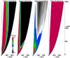 |
Fig. 2 Two-dimensional cuts of the calculated H2O gas-phase abundance relative to H nuclei in the four source models with the parameters given in Table 1 in the same order as in Fig. 1. The plotted dusty streamlines have launch radii ranging from the dust sublimation radius Rsub to 25 AU. Initial abundances at the wind base are discussed in Appendix D. The colour scale ranges from 10-6 to 10-4. |
In the densest model (extreme Class 0) the gas-phase water abundance stays constant along all dusty streamlines at the initial value of ≃10-4 because the disk wind is so dense that its dust content screens it efficiently against stellar FUV and X-rays photons, and water photodissociation is negligible. In the other three less dense models, photodissociation starts to operate and the evolution of the water abundance results from a competition between photodissociation and gas-phase reformation through the reaction OH + H2 → H2O + H. Since this reaction is endo-energetic by ≃1500 K, its speed increases not only with density, but also with temperature as exp(−1500 K/Tkin).
In the standard Class 0 model, FUV photodissociation remains moderate, but gas temperatures reach only a few hundred K so that reformation is not complete on scales of 2000 AU. The water abundance drops by typically 30% (x(H2O) ~ 3 × 10⁻⁵) on this scale. It reaches a minimum ~10-5 on intermediate streamlines launched from 3–6 AU, which are both less dense (i.e. slower reformation) than the axial regions and less well screened against FUV irradiation than the outermost streamlines.
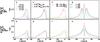 |
Fig. 3 Influence of our four free parameters on synthetic Herschel/HIFI profiles in the ortho-H2O fundamental line 110–101 at 557 GHz (top row) and the 312–221 line at 1153 GHz (bottom row). The reference profile (S0 model with |
In the Class 1 models, the wind is even more transparent than in the S0 model and FUV photodissociation of water is efficient above z/r ≃ 2 in the X1 model or right above the wind sonic point in the S1 model. At the same time the wind is warmer than in the S0 model, increasing the rate coefficient for water reformation. This allows a high water abundance ~10-4 to be maintained on the axial (densest) streamlines, while the abundance drops to ≤10-6 on outer streamlines where density is too low for reformation. Hence Class 1 models have their inner streamlines significantly more water-rich than outer ones, at variance with the shallower gradient predicted for the Class 0. We note that the axial spine of high water abundance extends to larger radii in the standard Class 1 compared to the extreme Class 1: the higher wind temperature in this case (see Fig. 1) makes reformation reactions more competitive than photodissociation.
3.3. Synthetic H O line profiles
Figure 3 illustrates the influence of our four free parameters (M⋆, Ṁacc, , i) on the predicted H2O line profiles in two lines of ortho-water: the fundamental 110–101 line at 557 GHz and the higher excitation 312−221 line at 1153 GHz. The 557 GHz line is selected for detailed study because it is the strongest water line, and the only one detected by WISH in Class 1 protostars and so it will provide our strongest basis for a statistical comparison with observations, including correlations with source properties (e.g. envelope density). The 1153 GHz line is among the most excited H2O lines detected with HIFI towards low-mass protostars, with an upper level at Eup ≃ 200 K above the fundamental level of ortho-water (see Sect. 4.2). We select it to investigate the influence of Eup on the emergent line profiles. In the excitation regime matching the observed line ratios in the BC, the excitation conditions probed by low-J water lines are found to depend only on the H2 density and H2O column density, with essentially no sensitivity to temperature above 300 K (see Fig. 11 of Mottram et al. 2014, and references therein). In our D-wind models, the regions dense enough to excite the 1153 GHz line are warmer than 300 K, hence the wind density and H2O column (set by its abundance) will also be the dominant factors determining the profile shape and intensity of this line, with only a small effect of the gas kinetic temperature.
As a reference case, in Fig. 3 we adopt the Standard Class 0 model (M⋆= 0.1 M⊙, Ṁacc= 5 × 10⁻⁶ M⊙ yr-1) with = 25 AU and i = 60°. We then overplot predicted profiles where only one of the four free parameters has been changed. A typical source distance of d = 235 pc (Perseus cloud) is adopted. We first present synthetic profiles for only one lobe of the disk wind (blue), as it makes it is easier to understand the origin of profile features. The result of adding the blue and red lobes is shown in the rightmost panel (together with the effect of changing inclination).
3.3.1. Changing the outermost launch radius r
Since the flow speed in our self-similar disk wind model scales as  (Keplerian law), one expects that the broad range of launch radii contributing to the emission in a disk wind will naturally produce a broad line profile. Figure 3 (panels a–b) illustrates how increasing from 3.2 to 25 AU indeed contributes to adding flux at progressively lower and lower velocity because of this scaling. As a result, a blue sloping wing develops while the red edge of the profile becomes steeper and steeper.
The quantitative effect of on the water line profile depends on the upper energy level. When increasing from 3.2 to 25 AU, the integrated line flux increases by a factor of ~2 in the fundamental 557 GHz line, and by only 30% for the 1153 GHz line. This occurs because the fundamental line (panel a) is more sensitive to the contribution of external streamlines than transitions from higher levels such as 312–221 (panel b), which require higher densities for excitation and are thus dominated by smaller r0. Hence, the fundamental line offers a better diagnostic of in the considered range.
We note that, in contrast to the total line intensity, the full width at zero intensity (FWZI) remains invariant to changes in because the FWZI is determined solely by the range of projected velocities along the fastest, innermost emitting streamline, here ejected from Rsub. In the reference case, the line pedestal of the blue jet lobe ranges from about −40 to +4 km s-1 when viewed at 60°. The blue edge corresponds to the maximum z-velocity (projected on the line of sight) reached along the Rsub streamline, while the red edge is produced by the initial rotation motions near the wind base.
3.3.2. Changing the accretion rate Ṁacc
Panels c, d of Fig. 3 present the effect of increasing the accretion rate by a factor of 4, from Ṁacc= 5 × 10⁻⁶ M⊙ yr-1 to 2 × 10⁻⁵ M⊙ yr-1, keeping all other reference parameters fixed. This modified set of parameters corresponds to our X0 source model in Table 1 where both the wind density and the hot-spot luminosity are multiplied by 4 from the reference S0 model.
The predicted profiles for X0 in Fig. 3c, d are divided by a factor of 5 to ease comparison with the reference S0 case. It can be seen that the main effect of increasing Ṁacc is to increase the intensity by a factor of ≃5 close to the density increase.
The shape of the profile wings is not strongly affected apart from a slight reduction of the maximum wing extension from −40 km s-1 to about −30 km s-1. This results from the four-fold increase in FUV hot-spot luminosity, which increases the sublimation radius Rsub from 0.31 to 0.63 AU and thus decreases the maximum velocity reached on the innermost Rsub streamline by the ratio of the Keplerian speeds ( ).
).
3.3.3. Changing the stellar mass M⋆
Panels e, f in Fig. 3 present the effect of increasing the stellar mass from 0.1 M⊙ to 0.5 M⊙, keeping all other reference parameters fixed. This modified set of (M⋆,Ṁacc) corresponds to our X1 source model in Table 1. The flow speed along each streamline V ∝ M⋆0.5 increases by a factor of ≃2, while the wind density ∝Ṁacc drops by the same factor; as a result, the H2O emission from each streamline is shifted to both higher radial velocity and lower intensity. Figure 3e, f shows that the two effects combine in such a way so as to produce a shape and intensity of the line wings that is very similar to the S0 model.
Figure 3e shows that the only clear difference between X1 and S0 profiles appears in the 557 GHz line at projected velocities below −20 km s-1 (for a view angle of 60°) where the X1 profile becomes flat-topped. This occurs because the slow outer streamlines that produced the strong central peaks in the X0 profile now become strongly photo-dissociated and water poor in the X1 model (see Fig. 2). This effect does not occur in the excited line at 1153 GHz as its emission is dominated by the wind base at z/r< 5 where H2O is not yet fully photodissociated. We note, however, that at higher inclination ≃80°, the flat-topped part of the 557 GHz line profile in the X1 model will shift to much lower velocities and become difficult to distinguish from the S0 557 GHz profile owing to the unknown envelope contribution at low velocities. This indicates that the fitting of observed profiles with our model grid will have some degeneracy unless there is an independent constraint on M⋆ or accretion age (Class) of the source.
3.3.4. Changing the inclination angle i
Panels g, h in Fig. 3 present the effect of varying the inclination angle i, with all other parameters set to their reference value. In order to prepare for the comparison with Herschel/HIFI observations in Sect. 4, we show here the “double sided” profiles obtained by summing the emission from the blueshifted and redshifted lobes of the disk wind.
In doing this summation we neglected radiative coupling between the two lobes (i.e. absorption of the red lobe by the blue lobe in front of it), the rationale being that at low inclinations ≤30° the two lobes are well separated in velocity and thus cannot absorb each other’s line emission, while at high inclinations ≥80° the two lobes are projected sufficiently well apart on the sky that they should suffer minimal overlap on each individual line of sight. This simplifying assumption may not be fully adequate at intermediate inclinations ≃60°. However, we stress that our main uncertainty in H2O profile predictions at low velocity is not the blue/red overlap, but the unknown envelope contribution (in emission or absorption) whose complex modeling lies well outside the scope of the present paper (see e.g. Schmalzl et al. 2014). Our comparison with observed HIFI line profiles will thus focus on the broad wing emission beyond ≃5 km s-1 from systemic, where the envelope contribution and blue/red overlaps should be minimal.
Figures 3g, h show that the main effect of increasing the inclination angle i is to reduce the base width of the line profile. This results from the cosi term involved in the projection of the maximum jet speed directed along the z-axis. The line width at zero intensity shrinks from ±60 km s-1 at 30° to ±20 km s-1 at i = 80°. This effect will allow us to constrain the inclination angle when comparing it with observed line profiles.
Another effect of observing farther away from pole-on is that it decreases the LVG line escape probability towards the line of sight, βlos, because of the smaller projected velocity gradient when looking at the jet sideways rather than down its axis. When the inclination increases from 30° to 80°, the integrated line intensity, ∫TdV , drops by a factor of 2.2 for the fundamental line at 557 GHz and by a factor of 1.7 for the excited line at 1153 GHz.
3.4. Scaling of ∫TdV with distance
In order to compare the intrinsic water line luminosity of protostellar objects observed at various distances d, it is often assumed that the observed ∫TdV scales as d-2 (e.g. Kristensen et al. 2012), meaning that the line flux comes mainly from an unresolved region. However, if the emission is unresolved across the flow axis but resolved and uniformly bright along the flow axis, ∫TdV will instead scale as d-1 (e.g. Mottram et al. 2014). We have thus investigated which scaling holds for our disk wind models, where the emission is centrally peaked but still somewhat extended.
We have calculated TdV for the 557 GHz and 1153 GHz lines in the Herschel beam for a range of source distances d< 100 to 400 pc and then fitted the results as a power law d− α. We find that the value of α depends mainly on the line excitation energy, the wind density, and the distance range, while and inclination have a smaller effect. The largest deviation from the point-source scaling is encountered in the fundamental 557 GHz line and for our highest value of Ṁacc = 2 × 10⁻⁵ (extreme Class 0 model), where the outer wind regions begin to contribute significantly. These regions start to be resolved at d< 100 pc where our fit yields α ≃ 1.3–1.4. However, for all larger distances d> 100 pc or smaller Ṁacc, we find that α ≃ 1.7–2. Lines from higher energy levels like 312–221 are dominated by denser and more compact jet regions than the fundamental line, and are thus seen as even more point-like with an α close to 2.
We conclude that if our disk wind model is adequate, using α = 2 is an acceptable approximation in most cases for the purpose of comparing the 557 GHz intrinsic brightness of sources at various distances and looking for global correlations with other parameters. Nevertheless, to determine the best-fitting grid parameters for each observed source, we will recompute synthetic line profiles at the corresponding source distance to minimize systematic effects.
4. Comparison with Herschel/HIFI H2O observations of protostars
We now compare our model predictions with the results of H2O rotational line profile observations towards 29 low-mass Class 0 and Class 1 protostars obtained with the HIFI spectrometer on board Herschel in the framework of the WISH key program (van Dishoeck et al. 2011). We explore whether our grid of dusty MHD disk wind models can reproduce the shape and intensity of the broad component of the fundamental H2O line at 557 GHz, as well as the correlation of its integrated intensity with envelope density found by Kristensen et al. (2012). We also investigate whether an MHD disk wind model can explain the relative intensities of more excited H2O lines.
4.1. The 557 GHz broad component profile
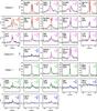 |
Fig. 4 Line profiles of the o-H2O fundamental line at 557 GHz towards 29 Class 0 and Class 1 low-mass protostars as observed with Herschel/HIFI (in black, from Kristensen et al. (2012)), superimposed with the closest matching line profile from our grid of 48 models (red = X0 model, pink = S0, green = X1, blue = S1). Predicted profiles were calculated for the specific distance and rest velocity of each source without any arbitrary intensity rescaling. The model parameters (source model, |
Grid models that best match the entire 557 GHz broad line wings.
Figure 4 compares the profile of the ortho-H2O fundamental line 110–101 at 557 GHz observed with Herschel/HIFI towards 29 low-luminosity Class 0 and Class 1 protostars by Kristensen et al. (2012) with the closest matching model among our grid of 48 cases. Adjustments were made on the broad wings of the central line component, excluding emission within ±5 km s-1 from systemic where the envelope contribution becomes significant. Each model was recomputed at the specific distance of each source and convolved by the 39′′ HIFI beam. No arbitrary rescaling of the model intensity was applied.
When both the S0 and X1 models gave equally acceptable adjustments (cf. Sect. 3.3.3), we favored the model consistent with the empirical source classification (Class 0 or Class 1) from the SED bolometric temperature Tbol as quoted by Kristensen et al. (2012). Figure 4 shows that a dusty MHD disk wind with values of Ṁacc and M⋆ typical of low-mass protostars, accretion age consistent with the source Class, and maximum launch radius in the range 3–25 AU can simultaneously reproduce to an impressive degree the shape, width, and intensity of at least one wing (and often both) of the broad central component of the 557 GHz line in all observed sources, except L1448-MM where the line wings are unusually broad2. This overall agreement between model and observations is especially noteworthy considering our use of only one MHD solution, and our sparse parameter grid.
Given our coarse grid, we note that the model adjustments in Fig. 4 should only be taken as illustrative examples of the ability of MHD disk winds to explain the broad component of the 557 GHz line in protostars and not as accurate determinations of M⋆, Ṁacc, i, and in each specific source. For example, the similarity between the S0 and X1 line wings seen in Fig. 3e demonstrates that there can be some degeneracy and that different parameter combinations could probably reproduce equally well or better the line profile in some cases. In the present exploratory study, we thus focus on the general trends of the model and do not attempt to refine the grid to provide optimal fits to each specific source. We also note that the value of used for the models plotted in Figure 4 is the maximum in our grid that is compatible with the observed line shape, but the true could be smaller if other physical components contribute to the inner line wings (e.g. a swept-up outflow cavity, reverse shock fronts in the wind). Table 3 summarizes the parameters of the plotted grid model for each source.
In three sources (Ced110-IRAS4, HH46-IRS, and NGC 1333-IRAS3 = SVS13) we were able to find a good fit only with a model of a different Class than indicated by their Tbol value. Their spectra are presented under the label “Class 0/1” in Fig. 4. We note that the same three sources stand out in the sample of Kristensen et al. (2012) as exhibiting envelope properties more typical of the other Class: HH46 and SVS13 have large envelop masses typical of Class 0 sources, while conversely Ced110-IRAS4 has the smallest envelope mass in the whole sample, smaller than all the sources classified as Class 1. Hence, these three sources may be borderline cases where the Tbol classification is ambiguous. For example, using the ratio of submm to bolometric luminosity as an alternative criterion would make Ced110-IRAS4 change from Class 0 to Class 1 (Lehtinen et al. 2001; André et al. 2000), in line with our modeling of its H2O line profile.
We did not attempt to reproduce the extremely high-velocity (EHV) “bullets” seen as discrete secondary peaks at ±25–50 km s-1 on either side of the central broad component in a few sources (BHR71, L1448-MM, and L1157). High-resolution studies of similar EHV bullets in SiO and CO have shown that they probe discrete internal shocks along the jet axis (e.g. Guilloteau et al. 1992; Santiago-García et al. 2009). Our steady disk wind model does not include shocks and thus cannot reproduce these features. The contribution of shocks might also explain why some sources show slight excess emission in one wing compared to our symmetric steady model, such as the blue wing in NGC 1333-IRAS 2A (see discussion in Sect. 4.2.1) and in Ser MM3. Alternatively, it may be possible that the ejection process is intrinsically asymmetric. Ser MM4 is a case in point, where the red and blue wings may be reproduced by disk wind models viewed at the same inclination and with the same stellar mass but with a different accretion rate and in either lobe.
4.2. Line profiles of excited HO lines
Another important test of the MHD disk wind model as a candidate for the broad component of the H2O 557 GHz line in protostars is whether it could also explain the component shape and intensity in lines of higher excitation. Sources from Fig. 4 with a rich dataset in this respect are the three Class 0 protostars in NGC 1333, and L1448-MM. We examine each of these sets in turn.
4.2.1. Class 0 protostars in NGC 1333
NGC 1333 IRAS 2A, IRAS 4A, and IRAS 4B are three well-studied prototypes of embedded Class 0 protostars in the Perseus complex (d = 235 pc). They were observed with Herschel/HIFI in several water lines by Kristensen et al. (2010). Figure 5 presents a comparison of all observed H2O line profiles in each source with synthetic predictions for our grid models that most closely match the fundamental 557 GHz profile (reproduced in the top row). The same models with a smaller are also shown as dashed curves.
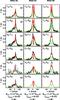 |
Fig. 5 Comparison of observed H2O line profiles (in black) towards NGC 1333-IRAS 2A, 4A, and 4B by Kristensen et al. (2010) with synthetic predictions (solid red curves) for the grid model best fitting the 557 GHz line in each source with parameters listed at the bottom. Predicted profiles for a smaller |
It can be seen that overall, the grid model that best matches the broad component of the 557 GHz line also reproduces remarkably well the wing intensity and shape in more excited H2O lines. Therefore, the excitation conditions in molecular magneto-centrifugal disk winds seem adequate to explain the broad component in excited H2O lines as well. The asymmetric blue wing in IRAS 2A, present in all lines, would trace an additional emission component not included in the steady disk wind model, e.g. shocks. The contribution of shocks to the blue wing H2O emission in IRAS2A is supported by the detection in the same velocity range of dissociative shock tracers in Herschel spectra (Kristensen et al. 2013) and of compact bullets along the jet in the interferometric map of Codella et al. (2014b).
4.2.2. L1448-MM
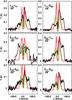 |
Fig. 6 Observed H2O line profiles towards L1448-MM (Kristensen et al. 2011) compared with synthetic predictions (in color) for the grid model best fitting the 557 GHz line (reproduced in the top left panel). Red solid curves are for |
L1448-MM in Perseus (d = 235 pc) is the first source where high-velocity bullets were detected (Bachiller et al. 1990), and where source characteristics were identified as pointing to an earlier evolutionary status than Class 1 sources (Bachiller et al. 1991), eventually leading to the introduction of the new Class 0 type (André et al. 1993). Figure 6 compares the six water line profiles observed with Herschel/HIFI towards L1448-MM by Kristensen et al. (2011) with predictions for the grid model best matching the 557 GHz line profile. As noted earlier, we do not attempt to reproduce the separate peaks centered at ±50 km s-1 (EHV bullets), which are known to trace internal shocks not included in our steady-state model, and we concentrate on the central broad component. While the modeled 557 GHz line wings are too narrow, the situation improves for lines of higher excitation. The evolution in relative peak intensities is also reproduced well by the model.
Figure 6 also shows that the weaker blue wing could be reproduced by a smaller = 3.2 AU than the red wing, where = 6.4 AU gives a good match. Alternatively, the intensity asymmetry between the blue and red wings could reflect different H2O abundances between the two lobes, caused for example by a different level of external FUV illumination. A possible extreme example of this effect is HH46-IRS, where the blue jet lobe is known to propagate out of the parent globule into a diffuse HII region, and the blue wing of the H2O 557 GHz profile is almost entirely lacking (cf. Fig 4).
4.3. Correlation of 557 GHz line luminosity with envelope density
Kristensen et al. (2012) searched for correlations in their sample between ∫TdV (200 pc), the integrated intensity of the 557 GHz line in the Herschel beam scaled to a distance of 200 pc (i.e. a quantity proportional to the line luminosity) and various intrinsic properties of the source. The tightest empirical correlation they obtained was with the envelope density at 1000 AU as determined by fitting the integrated source SED with the DUSTY 1D code. It is thus important to check whether our MHD disk-wind model could explain this good correlation and its slope close to 1. We note that the quantity denoted nH(1000 AU) in Kristensen et al. (2012) was actually the number density of H2 molecules (Kristensen, private communication). To avoid any ambiguity, here we use the notation  (1000 AU).
In Fig. 7 we plot as boxes the predicted locus of our four source models in the ∫TdV (200 pc)–(1000 AU) plane. The datapoints from Kristensen et al. (2012) are superimposed for comparison. The vertical range in ∫TdV (200 pc) for each model illustrates the effect of varying between 3.6 and 25 AU and the inclination between 80°and 30°. The horizontal range in envelope density plotted for each model is 1–3 times (1000 AU) (the fiducial envelope density given in Col. 4 of Table 1), i.e. it assumes an envelope in free fall onto the star of mass M⋆ at a rate that is 1–3 times the disk accretion rate Ṁacc.
First of all, Fig. 7 shows that the MHD disk wind model adopted here predicts a good correlation with a slope close to 1 between ∫TdV (200 pc) and the fiducial envelope density (1000 AU). The latter acts as a proxy for how the disk wind density changes from one model to the next (both quantities scaling as ṀaccM⋆-0.5). Hence this means that the modeled disk wind luminosity in the 557 GHz line is roughly proportional to the wind density (i.e. mass) inside the HIFI beam over a range of a factor of 45.
Second, Fig. 7 shows that the model predictions can reproduce very well the observed correlation and the dispersion among datapoints if (1000 AU) ≃1–3×(1000 AU); in other words, if the envelope free-fall rate measured at 1000 AU is ≃1–3 times the disk accretion rate in the MHD wind launching region inside 3–25 AU. Since the disk mass must increase early on, and the final mass of stars appears to be on average one-third of the initial core mass (André et al. 2010), such a relation between infall and accretion rates does not seem implausible in low-mass Class 0/1 sources.
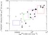 |
Fig. 7 Correlation between ∫TdV (200 pc), the integrated intensity in the 557 GHz line scaled to a distance of 200 pc, and |
5. Discussion
Our modeling results have shown that a model of dusty magneto-centrifugal disk wind is able to reproduce impressively well the range of shapes and intensities of the broad component of various H2O lines in low-mass Class 0 and Class 1 sources, as observed with HIFI/Herschel by Kristensen et al. (2012). It can also reproduce well the close correlation between 557GHz line intensity and envelope density discovered by these authors, provided the infall rate at 1000 AU is ≃1–3 times the disk accretion rate. As a consistency check, we now examine whether such an interpretation is compatible, at least in an average sense, with independent estimates of disk properties and system inclinations in low-mass protostars.
5.1. Disk radii in low-mass protostars
If the broad component of H2O in low-mass protostars does arise predominantly in a warm molecular MHD disk wind, the present exploratory models suggest that low-mass Class 0 and Class 1 protostars should all possess a Keplerian accretion disk, with sufficient magnetic flux to launch magneto-centrifugal ejection out to ≃3–25 AU. Pseudo-disks where motions are essentially radial rather than toroidal (due to magnetic braking on larger scales) would not be expected to generate enough magnetic twist to drive a powerful magneto-centrifugal outflow until the infalling matter approaches the centrifugal barrier. Here we briefly discuss whether this requirement seems consistent with the known Keplerian disk sizes in low-mass Class 0/1 protostars.
Direct observational evidence for Keplerian disks around embedded protostars has long been challenging to obtain because of heavy confusion with the dense infalling and rotating large-scale envelope. However, the continued improvement in angular resolution and sensitivity of radio interferometers has revealed several good candidates among both Class 1 and Class 0 sources (see the compilation in Table 7 of Harsono et al. 2014; and the more recent ALMA results of Sakai et al. 2014; Ohashi et al. 2014; Lee et al. 2014; Codella et al. 2014a).
The inferred outer radii for these Keplerian disks are generally 50–200 AU, comfortably larger than the maximum ejection radius ≃ 3−25 AU needed to reproduce the entire broad component of the H2O 557GHz line with the present MHD disk wind model (see Table 3). The most stringent constraint for our model is provided by the close binary system of L1551-IRS5 where individual circumstellar disks appear tidally truncated at an outer radius of only 8 AU (Lim & Takakuwa 2006). Our best grid model for L1551 has = 3.2 AU, which is consistent with this limit.
5.2. Disk accretion rates in low-mass protostars
Disk accretion rates in Class 0/1 protostars remain highly uncertain. In such embedded sources, empirical proxies for Lacc calibrated on Class 2 disks (FUV excess from the accretion shock, Brγ luminosity, etc.) suffer extremely high circumstellar extinction and scattering that cannot be accurately corrected for. Since the energy of absorbed FUV and near-IR photons is eventually re-emitted at longer wavelengths, the bolometric luminosity Lbol(integrated over all wavelengths) may offer a better proxy for the accretion luminosity Lacc in low-mass protostars. However, it still involves large uncertainties due to the unknown fraction εrad of accretion power that is actually radiated away instead of being used to drive ejection(s) or heat the star (Adams et al. 1987), and to the ill-known stellar photospheric contribution L⋆ in heavily accreting stars. An additional complication is that the dust radiation field is highly anisotropic due to disk inclination, occultation, and photon scattering in bipolar outflow cavities. Therefore, the observed spectral energy distribution (SED) will strongly depend on view angle (see e.g. Robitaille et al. 2007b), and the apparent Lbol obtained by multiplying by 4π the bolometric flux as seen from Earth (which is the only observed quantity) will differ from the true Lbol actually radiated by the source over all directions. For example, the apparent Lbol for L1551-IRS5 is 22 L⊙, but its SED can be well fitted by models with a true Lbol ranging from 7 L⊙ to 72 L⊙ (see Table 6 of Robitaille et al. 2007a), i.e. up to a factor of 3 smaller or larger than the apparent Lbol. The full uncertainty range in the true Lbol can reach a factor of 50–100 in some sources (see Table 6 of Robitaille et al. 2007a).
Computing angle-dependent SEDs for all our grid models would require complex 2D dust radiative transfer calculations and infalling envelope models that are well beyond the scope of the present work. For the sake of comparing our model-predicted disk accretion rates with observational constraints, we will assume that inclination effects affecting the apparent Lbol will tend to average out over a large sample so that the angle-averaged Lbol for our models will be close to the true Lbol. For the latter, we consider two simplified illustrative cases: (1) Lbol = 2 L⊙ + Lacc, corresponding to a photosphere of 2 L⊙ and 100% of the accretion luminosity eventually getting radiated (εrad = 1); and (2) Lbol = Lacc/2, corresponding to the situation where L⋆≪Lacc (true protostar) and the MHD disk wind extracts all the mechanical energy ≃0.5Lacc released by accretion through the Keplerian disk, while the rest is radiated by the hot spot (εrad = 0.5).
In Fig. 8, we plot as rectangles the predicted average location of our four source models in the ∫TdV (200 pc) – Lbol plane, for these two cases. It can be seen that they agree very well with the average Lbol values of the datapoints of Kristensen et al. (2012). Furthermore, it is striking that the systematic vertical shift between Class 0 and Class 1 sources observed in this graph is also reproduced well. This shift occurs in our disk-wind models because for a given Lacc, Class 0 sources have a 5 times smaller M⋆ and larger Ṁacc than Class 1 sources. Hence their disk wind is much denser (∝ṀaccM⋆-0.5) than in Class 1 sources of the same Lbol, and thus much brighter in the 557GHz line (cf. Fig. 7).
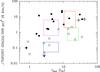 |
Fig. 8 Correlation between ∫TdV (200 pc), the integrated intensity in the 557 GHz line scaled to a distance of 200 pc, and Lbol, the apparent bolometric luminosity of the source. Data points from Kristensen et al. (2012) are marked according to their Tbol classification (filled = Class 0, open = Class 1). The borderline Class 0/Class 1 sources according to our model fits (see text) are indicated by a vertical cross. Colored rectangles illustrate the predicted loci of the four models in Table 1 for |
We note that the data points span a broader range of apparent Lbol than our model predictions. This is to be expected for several reasons. First, the angle-dependence of the dust radiation field (due to disk inclination and scattering in outflow cavities) will make the apparent Lbol differ by up to a factor of 3–10 (see discussion above) from the true Lbol that we have used to place our models in Fig. 8. Second, because Lacc is proportional to ṀaccM⋆, it is much more sensitive to a joint increase in both parameters than the H2O 557GHz luminosity, which scales as ≃ṀaccM⋆-0.5 (like the envelope density, see Sect. 4.3). For example, an increase in both Ṁacc and M⋆ by a factor of 2 will increase Lacc by a factor of 4, but will increase ∫TdV (200pc) by only  , i.e. 40%. Therefore, if the observed targets span a slightly broader range of Ṁacc and M⋆ than we have considered in our limited model grid (which is quite likely), a broader range of Lbol than our model predictions could also easily arise without affecting the predicted 557 GHz line luminosities very much. Finally, the accretion shock energy may not be entirely radiated away but used to drive a stellar wind that spins down the protostar (Matt & Pudritz 2008), in which case εrad ≪ 0.5 and the true Lbol for our models could extend to smaller values than the range plotted in Fig. 7. We conclude that the MHD disk wind models that reproduce the H2O broad line component in low-mass Class 0/1 protostars involve disk accretion rates that appear consistent on average with observational constraints, given the current observational and theoretical uncertainties in relating the apparent Lbol with the true Lacc.
5.3. Inclination angles
Although our very sparse parameter grid means that our line profile modeling is only illustrative, it is instructive to look at the statistical distribution of viewing angles suggested by the present modeling exercise. The behavior is quite different between Class 0 and Class 1 sources. Among the 16 sources best matched by our Class 0 grid models (including HH46-IRS and SVS13), the three inclination bins in our grid are equally represented (5–6 sources in each). In contrast, among the 13 sources best matched by our Class 1 grid models, only one is reproduced with i = 30° (TMC1A) and two with i = 60° (Oph-IRS63 and Ced 110), while the remaining ten require i = 80°. This reflects the trend for narrower H2O line wings in Class 1 sources already noted by Kristensen et al. (2012), Mottram et al. (2014). Our modeling confirms that this difference in line width between the two Classes is real and is not due to signal-to-noise issues; either the Class 1 sample is intrinsically poor in objects seen closer to pole-on (e.g. because these sources would look more like Class 2), or our disk-wind modeling in Class 1 sources predicts excessive H2O line widths, thus requiring artificially high inclinations to fit the observed line profiles.
To try and distinguish between these two possibilities, we have compared the inclinations of our best matching grid models with independent inclination estimates from jet proper motions (L1448-MM, IRAS4B, HH46-IRS, SVS13), radial velocity (IRAS15398), and bowshock modeling (L1551) or from modeling of the CO outflow kinematics and scattered light images (B335, L1157, L1527, GSS30, L1489, RNO91). These inclination values and the corresponding bibliographic references are listed in the last two columns of Table 3. Inclination estimates from the mere visual appearance of CO outflow lobes in single-dish maps were considered too uncertain for such a comparison because of the limited angular resolution3. Inclination estimates derived solely from fits to the source SED were also deemed too uncertain given the many free parameters involved (see e.g. Table 1 of Robitaille et al. 2007a) and the uncertainties in dust properties.
Among the 16 sources modeled by Class 0 profiles, 7 have independent inclination estimates and except for L1448-MM (which is not well fitted by any of our grid models) they are all consistent with our modeled inclination to within 10°, which is reassuring. Among the 13 sources modeled by Class 1 profiles, only 4 have direct inclination estimates: 35°–55° in L1551, 70° ± 4° in RNO91, ≃65° in GSS30, and ≥57° in L14894. The 557GHz line profiles of these four sources are all best matched by our Class 1 grid models with i = 80° (see Fig. 4). Hence, our Class 1 models do predict excessive inclination in two out of the four cases. Although the statistics are poor, they do suggest that our models for Class 1 sources seem to predict line wings that are slightly too broad. Several situations could lead to narrower line wings in Class 1 MHD disk winds than in our present models: (i) the initial H2O abundance on inner streamlines is smaller than assumed; (ii) the MHD ejection starts well beyond Rsub so that only slower streamlines emit in H2O; or (iii) the wind magnetic lever arm is smaller than in Class 0 sources, hence the wind is accelerated to lower speeds. Testing each of these options requires dedicated modeling that lies beyond the scope of the present exploratory work, and will be the subject of a forthcoming article.
6. Conclusions
The calculations presented in this paper show that the MHD disk wind model invoked to explain jet rotation in T Tauri stars, if launched from dusty accretion disks around low-mass Class 0 and Class 1 protostars, would be sufficiently warm, dense, and water rich to produce H2O emission detectable by HIFI on board the Herschel satellite. We find that the H2O line profiles predicted by this model reproduce the observational data remarkably well in spite of the sparse grid of parameters (Ṁacc M⋆ , inclination) that we have considered in our model grid. In particular, they can reproduce
-
the shape, velocity extent, and intensity of the broad component of the fundamental o-H2O line at 557 GHz;
-
the profiles and relative intensities of this broad component in more excited H2O lines;
-
the good correlation with a slope ≃1 between the H2O 557 GHz luminosity and the envelope density at 1000 AU;
-
the systematically higher water luminosity of Class 0 sources compared to Class 1 sources of the same bolometric luminosity.
These results indicate that MHD disk winds are an interesting option to consider for the origin of the broad H2O line component discovered by Kristensen et al. (2012) towards low-mass protostars with HIFI/Herschel. If this interpretation is correct, an important implication would be that all low-luminosity Class 0 protostars possess Keplerian accretion disks that are sufficiently magnetized out to 3–25 AU to launch MHD disk winds that extract a large fraction of the angular momentum necessary for accretion and have accretion rates on the order of 30%–100% of their envelope infall rate at 1000 AU.
In the case of Class 1 sources, their systematically narrower line wings in the 557 GHz line, first noted by Kristensen et al. (2012), would imply that they are mainly viewed close to edge-on (i ≃ 80°) or, more likely, that their MHD disk winds (if present) are less water rich and/or slower in their inner regions than the specific MHD solution used here.
Of course, the success of the MHD disk wind model explored here in fitting the broad component of HIFI/Herschel H2O line profiles does not mean that this model is necessarily correct or unique. Other possible origins for the broad component have been proposed that are not ruled out at this stage, such as shocked material or mixing-layers along the outflow cavity walls (see e.g. Mottram et al. 2014). Further tests of the disk wind hypothesis need to be undertaken in a range of molecular tracers (including e.g. CO J = 16–15 HIFI line profiles, Kristensen et al., in prep.) and with higher angular resolution. The revolutionary mapping sensitivity and angular resolution of the ALMA instrument are particularly well suited to searching for the slow and warm wide-angle component predicted by MHD disk wind models. Synthetic predictions for CO and early-science ALMA will be presented in a forthcoming paper and compared with available data.
Following the referee’s request, we have checked the effect of adopting more recent rates for these three types of reactions, which we obtained respectively from a compilation of the NIST Kinetics Database (kinetics.nist.gov), Neau et al. (2000), and van Dishoeck et al. (2006). We find that the predicted H2O emissivities are changed by less than 25% in regions that contribute significantly to emergent line profiles. Our modeling is certainly not accurate down to this level owing to the simplifications made to render the problem tractable (e.g. LVG approximation, 1D dust radiative transfer). Hence, the results obtained with the adopted chemical rates in Table 2 are still adequate for the purpose of this exploratory paper, which is to investigate the overall potential of our MHD disk wind model to explain the observed H2O profiles and correlations with source parameters, not to infer very precise quantities.
We see in Sect. 4.2.2 that the relative peak intensities among excited H2O lines in L1448-MM are still reproduced well by our model.
For example, Yıldız et al. (2012) suggest i = 15°–30° for IRAS4B, whereas proper motions ≃10–40 km s-1 and radial velocities ≃±8 km s-1 of H2O masers (Desmurs et al. 2009) indicate i = 50°–80° on small-scales. van Kempen et al. (2009) suggest that the CO outflow in IRAS15398 is viewed 15° from pole-on, whereas the low radial velocity ≃−46 km s-1 of the associated Herbig-Haro object (Heyer & Graham 1989) compared to typical jet speeds ≃150 km s-1 favors a high inclination from the line of sight, i ≥ 70°.
Brinch et al. (2007b) have argued that the high mid-infrared flux in L1489 requires a much smaller inclination for the disk (40°) than for the outflow cavities. However, their SED models do not include internal disk heating by accretion. Furthermore, the dust scattering efficiency at mid-infrared wavelengths would be much increased if large micron-sized grains are present, as suggested by the recent discovery of “coreshine” in dense cores (Pagani et al. 2010). Both effects would increase the predicted mid-IR disk flux and allow for a higher disk inclination
Acknowledgments
We are grateful to Simon Bruderer, Moshe Elitzur, David Flower, Lars Kristensen, Joe Mottram, and Laurent Pagani for useful discussion and advice at various stages of this work, and to the anonymous referee for constructive comments that helped to improve the paper. This work received financial support from the INSU/CNRS Programme National de Physique et Chimie du Milieu Interstellaire (PCMI), and made use of NASA’s Astrophysics Data System.
References
- Adams, F. C., Lada, C. J., & Shu, F. H. 1987, ApJ, 312, 788 [NASA ADS] [CrossRef] [Google Scholar]
- André, P., Ward-Thompson, D., & Barsony, M. 1993, ApJ, 406, 122 [NASA ADS] [CrossRef] [Google Scholar]
- André, P., Ward-Thompson, D., & Barsony, M. 2000, Protostars and Planets IV, 59 [Google Scholar]
- André, P., Men’shchikov, A., Bontemps, S., et al. 2010, A&A, 518, L102 [NASA ADS] [CrossRef] [EDP Sciences] [Google Scholar]
- Bachiller, R., Martin-Pintado, J., Tafalla, M., Cernicharo, J., & Lazareff, B. 1990, A&A, 231, 174 [NASA ADS] [Google Scholar]
- Bachiller, R., Andre, P., & Cabrit, S. 1991, A&A, 241, L43 [NASA ADS] [Google Scholar]
- Barber, R. J., Tennyson, J., Harris, G. J., & Tolchenov, R. N. 2006, MNRAS, 368, 1087 [NASA ADS] [CrossRef] [Google Scholar]
- Baruteau, C., Crida, A., Paardekooper, S.-J., et al. 2014, Protostars and Planets VI, 667 [Google Scholar]
- Blandford, R. D., & Payne, D. G. 1982, MNRAS, 199, 883 [NASA ADS] [CrossRef] [Google Scholar]
- Brinch, C., Crapsi, A., Hogerheijde, M. R., & Jørgensen, J. K. 2007a, A&A, 461, 1037 [NASA ADS] [CrossRef] [EDP Sciences] [Google Scholar]
- Brinch, C., Crapsi, A., Jørgensen, J. K., Hogerheijde, M. R., & Hill, T. 2007b, A&A, 475, 915 [Google Scholar]
- Cabrit, S., Goldsmith, P. F., & Snell, R. L. 1988, ApJ, 334, 196 [NASA ADS] [CrossRef] [Google Scholar]
- Cabrit, S., Ferreira, J., & Raga, A. C. 1999, A&A, 343, L61 [Google Scholar]
- Casse, F., & Ferreira, J. 2000, A&A, 361, 1178 [NASA ADS] [Google Scholar]
- Chrysostomou, A., Clark, S. G., Hough, J. H., et al. 1996, MNRAS, 278, 449 [NASA ADS] [Google Scholar]
- Codella, C., Cabrit, S., Gueth, F., et al. 2014a, A&A, 568, L5 [Google Scholar]
- Codella, C., Maury, A. J., Gueth, F., et al. 2014b, A&A, 563, L3 [NASA ADS] [CrossRef] [EDP Sciences] [Google Scholar]
- Cohen, N., & Westberg, K. R. 1983, J. Phys. Chem. Reference Data, 12, 531 [Google Scholar]
- Daniel, F., Dubernet, M.-L., & Grosjean, A. 2011, A&A, 536, A76 [NASA ADS] [CrossRef] [EDP Sciences] [Google Scholar]
- Desmurs, J.-F., Codella, C., Santiago-García, J., Tafalla, M., & Bachiller, R. 2009, A&A, 498, 753 [Google Scholar]
- Dubernet, M.-L., Daniel, F., Grosjean, A., & Lin, C. Y. 2009, A&A, 497, 911 [NASA ADS] [CrossRef] [EDP Sciences] [Google Scholar]
- Ferreira, J., Dougados, C., & Cabrit, S. 2006, A&A, 453, 785 [NASA ADS] [CrossRef] [EDP Sciences] [Google Scholar]
- Flower, D. R., & Pineau des Forêts, G. 2003, MNRAS, 343, 390 [NASA ADS] [CrossRef] [Google Scholar]
- Flower, D. R., & Pineau des Forêts, G. 2010, MNRAS, 406, 1745 [NASA ADS] [Google Scholar]
- Frank, A., Ray, T. P., Cabrit, S., et al. 2014, Protostars and Planets VI, 451 [Google Scholar]
- Garcia, P. J. V., Cabrit, S., Ferreira, J., & Binette, L. 2001a, A&A, 377, 609 [NASA ADS] [CrossRef] [EDP Sciences] [Google Scholar]
- Garcia, P. J. V., Ferreira, J., Cabrit, S., & Binette, L. 2001b, A&A, 377, 589 [NASA ADS] [CrossRef] [EDP Sciences] [Google Scholar]
- Girart, J. M., & Acord, J. M. P. 2001, ApJ, 552, L63 [NASA ADS] [CrossRef] [Google Scholar]
- Gredel, R., Lepp, S., Dalgarno, A., & Herbst, E. 1989, ApJ, 347, 289 [NASA ADS] [CrossRef] [Google Scholar]
- Gueth, F., Guilloteau, S., & Bachiller, R. 1996, A&A, 307, 891 [NASA ADS] [Google Scholar]
- Guilloteau, S., Bachiller, R., Fuente, A., & Lucas, R. 1992, A&A, 265, L49 [NASA ADS] [Google Scholar]
- Harsono, D., Jørgensen, J. K., van Dishoeck, E. F., et al. 2014, A&A, 562, A77 [NASA ADS] [CrossRef] [EDP Sciences] [Google Scholar]
- Hartigan, P., Morse, J., Palunas, P., Bally, J., & Devine, D. 2000, AJ, 119, 1872 [NASA ADS] [CrossRef] [Google Scholar]
- Hartigan, P., Heathcote, S., Morse, J. A., Reipurth, B., & Bally, J. 2005, AJ, 130, 2197 [NASA ADS] [CrossRef] [Google Scholar]
- Heyer, M. H., & Graham, J. A. 1989, PASP, 101, 816 [NASA ADS] [CrossRef] [Google Scholar]
- Hincelin, U., Wakelam, V., Commerçon, B., Hersant, F., & Guilloteau, S. 2013, ApJ, 775, 44 [NASA ADS] [CrossRef] [Google Scholar]
- Ivezic, Z., & Elitzur, M. 1997, MNRAS, 287, 799 [NASA ADS] [CrossRef] [Google Scholar]
- Konigl, A., & Pudritz, R. E. 2000, Protostars and Planets IV, 759 [Google Scholar]
- Kristensen, L. E., Visser, R., van Dishoeck, E. F., et al. 2010, A&A, 521, L30 [NASA ADS] [CrossRef] [EDP Sciences] [Google Scholar]
- Kristensen, L. E., van Dishoeck, E. F., Tafalla, M., et al. 2011, A&A, 531, L1 [Google Scholar]
- Kristensen, L. E., van Dishoeck, E. F., Bergin, E. A., et al. 2012, A&A, 542, A8 [NASA ADS] [CrossRef] [EDP Sciences] [Google Scholar]
- Kristensen, L. E., van Dishoeck, E. F., Benz, A. O., et al. 2013, A&A, 557, A23 [NASA ADS] [CrossRef] [EDP Sciences] [Google Scholar]
- Lee, C.-F., Mundy, L. G., Reipurth, B., Ostriker, E. C., & Stone, J. M. 2000, ApJ, 542, 925 [NASA ADS] [CrossRef] [Google Scholar]
- Lee, C.-F., Hirano, N., Zhang, Q., et al. 2014, ApJ, 786, 114 [NASA ADS] [CrossRef] [Google Scholar]
- Lefloch, B., Cabrit, S., Busquet, G., et al. 2012, ApJ, 757, L25 [NASA ADS] [CrossRef] [Google Scholar]
- Lehtinen, K., Haikala, L. K., Mattila, K., & Lemke, D. 2001, A&A, 367, 311 [NASA ADS] [CrossRef] [EDP Sciences] [Google Scholar]
- Li, Z.-Y., Banerjee, R., Pudritz, R. E., et al. 2014, Protostars and Planets VI, 173 [Google Scholar]
- Lim, J., & Takakuwa, S. 2006, ApJ, 653, 425 [NASA ADS] [CrossRef] [Google Scholar]
- Machida, M. N., & Hosokawa, T. 2013, MNRAS, 431, 1719 [NASA ADS] [CrossRef] [Google Scholar]
- Matt, S., & Pudritz, R. E. 2008, ApJ, 681, 391 [NASA ADS] [CrossRef] [Google Scholar]
- Millar, T. J., Bennett, A., & Herbst, E. 1989, ApJ, 340, 906 [NASA ADS] [CrossRef] [Google Scholar]
- Mottram, J. C., Kristensen, L. E., van Dishoeck, E. F., et al. 2014, A&A, 572, A21 [NASA ADS] [CrossRef] [EDP Sciences] [Google Scholar]
- Neau, A., Al Khalili, A., Rosén, S., et al. 2000, J. Chem. Phys., 113, 1762 [NASA ADS] [CrossRef] [Google Scholar]
- Nenkova, M., Ivezic, Z., & Elitzur, M. 1999, LPI Contributions, 969, 20 [NASA ADS] [Google Scholar]
- Neufeld, D. A., & Kaufman, M. J. 1993, ApJ, 418, 263 [NASA ADS] [CrossRef] [Google Scholar]
- Noriega-Crespo, A., & Garnavich, P. M. 2001, AJ, 122, 3317 [NASA ADS] [CrossRef] [Google Scholar]
- Ohashi, N., Saigo, K., Aso, Y., et al. 2014, ApJ, 796, 131 [NASA ADS] [CrossRef] [Google Scholar]
- Pagani, L., Steinacker, J., Bacmann, A., Stutz, A., & Henning, T. 2010, Science, 329, 1622 [NASA ADS] [CrossRef] [PubMed] [Google Scholar]
- Panoglou, D., Cabrit, S., Pineau des Forêts, G., et al. 2012, A&A, 538, A2 [NASA ADS] [CrossRef] [EDP Sciences] [Google Scholar]
- Pesenti, N., Dougados, C., Cabrit, S., et al. 2004, A&A, 416, L9 [NASA ADS] [CrossRef] [EDP Sciences] [Google Scholar]
- Robitaille, T., Whitney, B., Indebetouw, R., & Wood, K. 2007a, ApJS, 169, 328 [NASA ADS] [CrossRef] [Google Scholar]
- Robitaille, T., Whitney, B., Indebetouw, R., Wood, K., & Denzmore, P. 2007b, ApJS, 167, 256 [Google Scholar]
- Safier, P. N. 1993, ApJ, 408, 115 [NASA ADS] [CrossRef] [Google Scholar]
- Sakai, N., Sakai, T., Hirota, T., et al. 2014, Nature, 507, 78 [NASA ADS] [CrossRef] [Google Scholar]
- Santangelo, G., Nisini, B., Giannini, T., et al. 2012, A&A, 538, A45 [NASA ADS] [CrossRef] [EDP Sciences] [Google Scholar]
- Santiago-García, J., Tafalla, M., Johnstone, D., & Bachiller, R. 2009, A&A, 495, 169 [NASA ADS] [CrossRef] [EDP Sciences] [Google Scholar]
- Sauty, C., & Tsinganos, K. 1994, A&A, 287, 893 [NASA ADS] [Google Scholar]
- Schmalzl, M., Visser, R., Walsh, C., et al. 2014, A&A, 572, A81 [NASA ADS] [CrossRef] [EDP Sciences] [Google Scholar]
- Sheikhnezami, S., Fendt, C., Porth, O., Vaidya, B., & Ghanbari, J. 2012, ApJ, 757, 65 [NASA ADS] [CrossRef] [Google Scholar]
- Shu, F., Najita, J., Ostriker, E., et al. 1994, ApJ, 429, 781 [NASA ADS] [CrossRef] [Google Scholar]
- Sobolev, V. V. 1957, Sov. Astron., 1, 332 [NASA ADS] [Google Scholar]
- Surdej, J. 1977, A&A, 60, 303 [NASA ADS] [Google Scholar]
- Tennyson, J., Zobov, N. F., Williamson, R., Polyansky, O. L., & Bernath, P. F. 2001, J. Phys. Chem. Reference Data, 30, 735 [Google Scholar]
- Tobin, J. J., Hartmann, L., Calvet, N., & D’Alessio, P. 2008, ApJ, 679, 1364 [NASA ADS] [CrossRef] [Google Scholar]
- Turner, N. J., Fromang, S., Gammie, C., et al. 2014, Protostars and Planets VI, 411 [Google Scholar]
- van Dishoeck, E. F. 1988, in Rate Coefficients in Astrochemistry, eds. T. J. Millar, & D. A. Williams, Astrophys. Space Sci. Libr., 146, 49 [Google Scholar]
- van Dishoeck, E. F., Jonkheid, B., & van Hemert, M. C. 2006, Faraday Discussions, 133, 231 [NASA ADS] [CrossRef] [PubMed] [Google Scholar]
- van Dishoeck, E. F., Kristensen, L. E., Benz, A. O., et al. 2011, PASP, 123, 138 [NASA ADS] [CrossRef] [Google Scholar]
- van Kempen, T. A., van Dishoeck, E. F., Hogerheijde, M. R., & Güsten, R. 2009, A&A, 508, 259 [Google Scholar]
- Visser, R., van Dishoeck, E. F., Doty, S. D., & Dullemond, C. P. 2009, A&A, 495, 881 [NASA ADS] [CrossRef] [EDP Sciences] [Google Scholar]
- Yıldız, U. A., Kristensen, L. E., van Dishoeck, E. F., et al. 2012, A&A, 542, A86 [NASA ADS] [CrossRef] [EDP Sciences] [Google Scholar]
- Yıldız, U. A., Kristensen, L. E., van Dishoeck, E. F., et al. 2013, A&A, 556, A89 [NASA ADS] [CrossRef] [EDP Sciences] [Google Scholar]
- Zanni, C., & Ferreira, J. 2013, A&A, 550, A99 [NASA ADS] [CrossRef] [EDP Sciences] [Google Scholar]
Appendix A: H2 and CO self-shielding
One improvement in our model calculations since Panoglou et al. (2012) consists in the implementation of an accurate estimation of the shielding column of H2 molecules along the line of sight to the star, NH2. We now calculate the streamlines evolution in increasing order of launching radius r0, starting from the dust sublimation radius Rsub, where we assume NH2 = 0. The increment in H2 column density between two consecutive streamlines i − 1 and i at each polar angle θ is approximated by  (A.1)where xH2(i − 1,θ) is the fractional abundance of H2 at angle θ on the (i − 1)th streamline, and ΔNH(i,θ) is the increment in column density of H nuclei between streamlines i − 1 and i along angle θ. We use the H2 abundance on streamline i − 1 rather than some average value between the two consecutive streamlines because we found that an average leads to overestimating the shielding when the gradient in xH2 is steep, which will be the case near the H-H2 transition.
As we refine the spacing between successive streamlines, the variation of xH2(i,θ) as a function of r0 converges to a limiting curve, as illustrated in Fig. A.1 in the case of our reference S0 model. The final adopted discretization in r0 results from a trade-off between accuracy in xH2 and CPU time. The same method is applied to calculate the shielding column of CO molecules along the line of sight to the star, NCO.
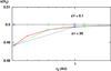 |
Fig. A.1 Effect of a finer sampling in streamline radii r0 on the calculated fractional H2 abundance xH2 = n(H2)/nH at the recollimation point (z/r = 20) of each streamline for our reference S0 model. We note the convergence to a limiting curve as the sampling is increased and the calculation of the self-shielding H2 column becomes more accurate. |
Appendix B: H2O rotational excitation and gas heating/cooling
The out-of-equilibrium evolution of H2O rotational level populations along each streamline is calculated under the large velocity gradient (LVG) approximation (Sobolev 1957) using the method developed for planar C-shocks by Flower & Pineau des Forêts (2010). We consider the first 90 rotational levels of H2O (45 ortho and 45 para), with energies up to 2 000 K taken from Tennyson et al. (2001), and their coupling by 320 radiative transitions with Aij from Barber et al. (2006). The rate coefficients adopted for collisions with He and H are the same as in Flower & Pineau des Forêts (2010). For collisions with H2 we use the more recent rate coefficients computed by Dubernet et al. (2009), Daniel et al. (2011). When the kinetic temperature exceeds the range where the coefficients are calculated, we use the last tabulated value. The rate of gas cooling/heating by H2O is calculated self-consistently with the local H2O level populations, as the net rate of energy lost/gained by the gas through H2O collisional excitation or de-excitation. This differs from Paper I, where cooling by H2O was evaluated from the tabulated LVG cooling functions of Neufeld & Kaufman (1993).
Unlike the shock models of Flower & Pineau des Forêts (2010), the disk wind is not plane-parallel. Hence the variation of photon escape probability with angle must be evaluated numerically. The projected velocity gradient  in each direction (θ1,φ1) is calculated numerically by interpolating the velocity field in the MHD solution. The Sobolev optical depth of the transition u → l in this direction is given by (see e.g. Surdej 1977)
 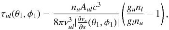 (B.1)where g and n denote the level statistical weight and number population, and νul and Aul are the transition frequency and spontaneous radiative decay rate. The corresponding photon escape probability is β(θ1,φ1) = (1−e− τul) /τul. A few lines occasionally show a maser effect with τul< 0, so that βul becomes greater than 1. Since the LVG treatment does not include maser saturation, we impose in this case an arbitrary upper limit of βmax = 5. However, this occurs only in very few directions and positions, and does not affect the emergent spectra.
The mean escape probability ⟨ β ⟩ averaged over all solid angles is obtained from Gaussian integration of β(θ1,φ1) over 12 values in θ1 and 12 values in φ1. The mean radiation field at the line frequency is then calculated with the usual LVG formula (e.g. Surdej 1977)  (B.2)where Tex is the excitation temperature of the transition, and
  is the background radiation field at the line frequency. The latter is taken equal to
  , the diffuse radiation field in the dusty disk wind as computed by the DUSTY code (see Appendix C). The value of
  is then used to calculate the rates of change of the level populations by stimulated emission and absorption, and evolve them to the next point in z along the streamline. The calculated escape probability in each direction (θ1,φ1) is saved and used to compute the contribution of each gas cell to the final emergent spectra.
Appendix C: Dust temperature and diffuse background
In Paper I, the grain temperature was computed from radiation equilibrium against the direct stellar and hot-spot radiation, attenuated by intervening dusty wind streamlines. This method is valid as long as the dust is optically thin to its own infrared radiation, an assumption that is not fully adequate in the dense winds from Class 1 and Class 0 sources, where backwarming becomes significant. We now include this effect in an approximate way, using the 1D radiative transfer code DUSTY (Nenkova et al. 1999). We adopt the same standard MRN grain composition, optical properties and size distribution as in Paper I. We approximate the density of H nuclei in the wind as a 1D power-law distribution nH(r,θ) ≃ 1/20 × (R), which provides a good approximation over the intermediate streamline region between the base and the recollimation point. Here R is the spherical radius and is the fiducial H2 density in a spherical envelope in free fall at rate Ṁacc onto a point source of mass M⋆![Mathematical equation: \appendix \setcounter{section}{3} \begin{eqnarray} n_\mathrm{H_2}^{\rm acc}(R) & \equiv &\frac{1}{2} \frac{\mMacc R^{-1.5}}{4 \pi \mu m_\mathrm{p} \sqrt{2 G \mMstar}} \nonumber\\[1.2mm] &\simeq& 6 \times 10^5 {\rm cm}^{-3} \left(\frac{\mMacc}{5\times 10^{-6} \UMacc} \right) \left(\frac{\mMstar} {0.1 M_\odot} \right)^{-0.5} \nonumber\\[1mm] & & \times \left(\frac{R}{1000\, \AU} \right)^{-1.5} \label{eq:nff} , \end{eqnarray}](/articles/aa/full_html/2016/01/aa25915-15/aa25915-15-eq238.png) (C.1)where μ = 1.4 accounts for the mass in the form of helium.
(C.1)where μ = 1.4 accounts for the mass in the form of helium.
We take the inner radius of the 1D dust shell to be at the sublimation radius, denoted Rsub, where Td= 1500 K. The dust is heated by a central source made of two blackbodies, a stellar photosphere of 2 L⊙ at 4000 K, and an accretion shock at 10 000 K radiating half of the accretion luminosity (see Paper I for a discussion of these assumptions). The calculated dust sublimation radius is listed in Table 1 for our four source models. It is ≃0.3AU in models S0 and S1 (50% larger than in Paper I), and ≃0.6AU in models X0 and X1. Visser et al. (2009) carried out full 2D dust radiative transfer calculations in a rotating collapsing singular isothermal sphere and found that the disk surface reaches a dust temperature of 100 K out to 17–41 AU in their reference and standard models. For comparison, we find Td = 100 K at 25–80 AU in our 1D DUSTY calculations for a comparable source luminosity. The use of an approximate 1D dust radiative transfer thus appears sufficiently accurate for our purposes, given the other simplifying hypotheses in our model and the exploratory nature of our work.
The DUSTY code also calculates the local angle-averaged specific intensity  (see Eq. (C.1) in Ivezic & Elitzur 1997). It includes the submillimeter diffuse radiation emitted by warm dust grains, as well as the attenuated and geometrically diluted contribution of the star and hot spots at shorter wavelengths. This background radiation field is taken into account in computing the H2O rotational level excitation, as discussed in Appendix B.
Appendix D: Initial conditions at the wind base
In Paper I, the initial temperature and chemical abundances at the base of each streamline were obtained in a simple way by calculating the local steady-state thermochemical equilibrium (reached typically after 3 × 10⁵ yrs). Although convenient, this procedure did not take into account the previous chemical history of the gas as it was accreted from larger radii up to the current r0. When the disk angular momentum is mainly extracted by MHD wind torques (as in the MHD solution adopted here), the accretion flow is much faster than in a viscous disk and typically transonic with Vacc ≃ 0.7Cs, where the sound speed Cs is related to the Keplerian speed through Cs = (h/r0)VKep(r0). The disk aspect ratio h/r0 ≡ ϵ is constant in our self-similar model, with a value of 0.03. As a consequence, the characteristic
radial drift timescale tacc at distance r0 from the star is 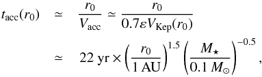 (D.1)which is much shorter than the timescale to reach chemical equilibrium.
Computing the full 2D non-equilibrium chemical evolution along the accretion flow is a highly complex problem that represents a full work in its own right Visser et al. (2009), Hincelin et al. (2013). For the purpose of the present exploratory paper, we adopt the following simpler approach to estimating chemical abundances at the wind slow point. We first start from typical steady-state dark cloud conditions with the ice phase composition of Flower & Pineau des Forêts (2003) and evolve the gas-phase chemical abundances at r0 = 50 AU for a duration of 3 × 10⁵ yr, typical of the viscous accretion time in the outer disk where ionization is too low for MHD ejection to take place. This is sufficient to reach chemical steady state, hence the result does not depend on the precise adopted duration. We then propagate the resulting abundances at the wind slow point at r0 = 25 AU, putting back in the gas phase all ice species that are thermally desorbed (Td≥ 100 K), and to mimic the effect of accretion we evolve the abundances and gas temperature at the local density nH(25 AU) for a short duration equal to the accretion timescale tacc(r0) given by Eq. (D.1). The result is taken as initial conditions for the thermo-chemical integration along the 25 AU wind streamline. We then proceed in the same way at the next smaller r0 = 12.8 AU, using the calculated abundances at the slow point at 25 AU as input and evolving them for a duration tacc(r0) to obtain the initial conditions for the thermo-chemical integration along that wind streamline. We progress recursively in this way from outside in, down to r0 =Rsub.
Table D.1 summarizes the calculated initial gas and dust temperatures and H2O gas-phase abundance at the disk-wind slow point on a few representative streamlines for the standard Class 0 model, together with the local H nucleus density (imposed by the MHD solution). The main difference from Paper I is that the higher dust temperature, and ensuing ice thermal evaporation leads to a water gas-phase abundance of about 10-4 at all launch radii ≤25 AU. When the gas temperature exceeds 250 K, additional water forms by endo-energetic reaction of O and OH with H2, but the accretion timescale is too short for this conversion to be complete. Similar initial water gas-phase abundances are found for the other three source models in Table 1.
Initial conditions at the wind slow point for the standard Class 0 model.
All Tables
All Figures
|
Fig. 1 Two-dimensional cuts of the calculated gas kinetic temperature (on a log10 scale) in the four source models with the parameters given in Table 1. The black contour levels are at 250, 400, 800, and 1600 K. The streamlines have launch radii ranging from the sublimation radius Rsub to 25 AU. The calculations were stopped inside the cone with z/r = 20 where streamlines start to recollimate towards the axis and shocks may later develop. The wind density drops from right to left successively by a factor 4, |
| In the text | |
|
Fig. 2 Two-dimensional cuts of the calculated H2O gas-phase abundance relative to H nuclei in the four source models with the parameters given in Table 1 in the same order as in Fig. 1. The plotted dusty streamlines have launch radii ranging from the dust sublimation radius Rsub to 25 AU. Initial abundances at the wind base are discussed in Appendix D. The colour scale ranges from 10-6 to 10-4. |
| In the text | |
|
Fig. 3 Influence of our four free parameters on synthetic Herschel/HIFI profiles in the ortho-H2O fundamental line 110–101 at 557 GHz (top row) and the 312–221 line at 1153 GHz (bottom row). The reference profile (S0 model with |
| In the text | |
|
Fig. 4 Line profiles of the o-H2O fundamental line at 557 GHz towards 29 Class 0 and Class 1 low-mass protostars as observed with Herschel/HIFI (in black, from Kristensen et al. (2012)), superimposed with the closest matching line profile from our grid of 48 models (red = X0 model, pink = S0, green = X1, blue = S1). Predicted profiles were calculated for the specific distance and rest velocity of each source without any arbitrary intensity rescaling. The model parameters (source model, |
| In the text | |
|
Fig. 5 Comparison of observed H2O line profiles (in black) towards NGC 1333-IRAS 2A, 4A, and 4B by Kristensen et al. (2010) with synthetic predictions (solid red curves) for the grid model best fitting the 557 GHz line in each source with parameters listed at the bottom. Predicted profiles for a smaller |
| In the text | |
|
Fig. 6 Observed H2O line profiles towards L1448-MM (Kristensen et al. 2011) compared with synthetic predictions (in color) for the grid model best fitting the 557 GHz line (reproduced in the top left panel). Red solid curves are for |
| In the text | |
|
Fig. 7 Correlation between ∫TdV (200 pc), the integrated intensity in the 557 GHz line scaled to a distance of 200 pc, and |
| In the text | |
|
Fig. 8 Correlation between ∫TdV (200 pc), the integrated intensity in the 557 GHz line scaled to a distance of 200 pc, and Lbol, the apparent bolometric luminosity of the source. Data points from Kristensen et al. (2012) are marked according to their Tbol classification (filled = Class 0, open = Class 1). The borderline Class 0/Class 1 sources according to our model fits (see text) are indicated by a vertical cross. Colored rectangles illustrate the predicted loci of the four models in Table 1 for |
| In the text | |
|
Fig. A.1 Effect of a finer sampling in streamline radii r0 on the calculated fractional H2 abundance xH2 = n(H2)/nH at the recollimation point (z/r = 20) of each streamline for our reference S0 model. We note the convergence to a limiting curve as the sampling is increased and the calculation of the self-shielding H2 column becomes more accurate. |
| In the text | |
Current usage metrics show cumulative count of Article Views (full-text article views including HTML views, PDF and ePub downloads, according to the available data) and Abstracts Views on Vision4Press platform.
Data correspond to usage on the plateform after 2015. The current usage metrics is available 48-96 hours after online publication and is updated daily on week days.
Initial download of the metrics may take a while.