| Issue |
A&A
Volume 585, January 2016
|
|
|---|---|---|
| Article Number | A154 | |
| Number of page(s) | 11 | |
| Section | Interstellar and circumstellar matter | |
| DOI | https://doi.org/10.1051/0004-6361/201425409 | |
| Published online | 14 January 2016 | |
The H i supershell GS 118+01−44 and its role in the interstellar medium
1
Instituto Argentino de Radioastronomía (CCT-La Plata,
CONICET), CC 5, 1894,
Villa Elisa,
Argentina
e-mail: This email address is being protected from spambots. You need JavaScript enabled to view it.
2
Instituto de Astronomía y Física del Espacio (CONICET-UBA), Cuidad
Universitaria, C.A.B.A, Argentina
3 Space Telescope Science Institute, 3700 San Martin Drive,
Baltimore DM 21218,
USA
4
Facultad de Ciencias Astronómicas y Geofísicas, Universidad
Nacional de La Plata, La
Plata, Argentina
5
Canada-France-Hawaii Telescope Corporation, 65-1238 Mamalahoa
Hwy, Kamuela,
HI
96743,
USA
Received:
26
November
2014
Accepted:
16
October
2015
Abstract
Aims. We carry out a multiwavelength study to characterize the H i supershell designated GS 118+01−44, and to analyse its possible origin.
Methods. A multiwavelength study has been carried out to study the supershell and its environs. We performed an analysis of the H i, CO, radio continuum, and infrared emission distributions.
Results. The Canadian Galactic Plane Survey (CGPS) H i data reveals that GS 118+01−44 is centred at (l,b) = (117°̣7, 1°̣4) with a systemic velocity of −44.3 km s-1. According to Galactic rotation models this structure is located at 3.0 ± 0.6 kpc from the Sun. There are several H ii regions and three supernova remnants (SNRs) catalogued in the region. On the other hand, the analysis of the temperature spectral index distribution shows that in the region there is a predominance of non-thermal emission. Infrared emission shows that cool temperatures dominate the area of the supershell. Concerning the origin of the structure, we found that even though several OB stars belonging to Cas OB5 are located in the interior of GS 118+01−44, an analysis of the energy injected by these stars through their stellar winds indicates that they do not have sufficient energy to create GS 118+01−44. Therefore, an additional energy source is needed to explain the genesis of GS 118+01−44. On the other hand, the presence of several H ii regions and young stellar object candidates in the edges of GS 118+01−44 shows that the region is still active in forming new stars.
Key words: ISM: bubbles / ISM: kinematics and dynamics / Hiiregions / stars: formation
© ESO, 2016
1. Introduction
Although few in number compared with low-mass stars, massive stars, defined as those stars with a main-sequence mass of at least 8 M⊙, are extremely important with regard to the physical and chemical conditions prevailing in the interstellar medium (ISM). Their importance stems from their UV ionizing radiation and energetic winds, which give rise to expanding H ii regions and interstellar bubbles. As a consequence of stellar evolution, supernova explosions take place within these expanding features, and these supernovae further contribute to the expansion of existing structures originating in previous stellar evolutionary stages. Since massive stars tend to be gregarious (e.g. as in an OB association), their cumulative effects may be one of the mechanisms at work, which may give rise to large scale structures known as supershells. Since these structures are mostly observed in the 21 cm line emission of the neutral hydrogen (H i) as regions of low H i emission surrounded, totally or partially, by walls of enhanced H i emission, they are usually referred to as H i supershells.
The first catalogue of Galactic H i shells/supershells was published by Heiles (1979). Later, based on different identification criteria, and making use of diverse H i databases, several additional catalogues were published (McClure-Griffiths et al. 2002; Ehlerová & Palouš 2005, 2013). These H i structures were also detected in nearby galaxies (Bagetakos et al. 2011). Recently, using a combination of a traditional identification criteria and an automatic algorithm procedure, 566 H i supershell candidates were identified in the second and third Galactic quadrants (Suad et al. 2014).
As the shells/supershells evolve in the ISM, the physical conditions for generating new stars can be fulfilled. Studies have been performed showing several cases of triggered star formation (e.g. Arnal & Corti 2007; Suad et al. 2012; Cichowolski et al. 2014). Although H i supershells are believed to be of importance in determining some large scale properties of the host galaxy (e.g. the gas injection into the lower Galactic halo), their origin and the role played by these structures in triggering star formation is a matter of debate.
In this paper, we present a comprenhesive study of one of the supershells detected in the catalogue of Suad et al. (2014), designated as GS 118+01−44. We analyse the atomic, molecular, radio continuum, and infrared emission in the region, trying to disentangle the origin of this large structure and its interaction with the ISM.
2. Observations
High angular resolution H i data were retrieved from the Canadian Galactic Plane Survey (Taylor et al. 2003, CGPS). Besides the high-resolution H i data, the CGPS also provides high-resolution continuum data at 408 and 1420 MHz (Landecker et al. 2000). The CGPS data base also comprises other data sets that have been reprojected and regridded to match the DRAO images. Among them is the Five College Radio Astronomical Observatory (FCRAO) CO Survey of the Outer Galaxy (Heyer et al. 1998).
Mid-infrared emission at 12 and 22 μm were obtained from the Wide-field Infrared Survey Explorer (WISE; Wright et al. 2010). These data were taken from the Nasa/IPAC Infrared Science Archive (IRSA) home page1.
Far-infrared emission at 65, 90, 140, and 160 μm were retrieved from the AKARI satellite (Takita et al. 2015). We also used Herschel (PACS) 160 μm data (red channel; Molinari et al. 2010) and Planck 350 and 550 μm data (Planck Collaboration I 2015). In Table 1 all the observational parameters are listed.
Observational parameters.
3. H i emission distribution
3.1. Previous H I works towards l ~ 118°
Fich (1986), using the H i database of Weaver & Williams (1973), reported an H i supershell likely to be associated with three Galactic supernova remnants. This feature, centred at (l,b) = (117.̊5, 1.̊5), is detected along the velocity range from −60 to −35 km s-1, and is ellipsoidal in shape with a major and minor axis of about 7° and ~3° in Galactic longitude and latitude, respectively.
Later, Moór & Kiss (2003), using the Leiden-Dwingeloo H i survey (Hartmann & Burton 1997), detected a large H i circular feature with an angular diameter of ~8.̊5, covering the velocity range from −60 to +3 km s-1 and centred at (l,b) = (117.̊5, 1.̊0). The authors suggest that this structure was created by the interaction of the massive stars of Cas OB5 with their surrounding ISM.
Later on, Cichowolski et al. (2009), using the CGPS database (Taylor et al. 2003), reported that the H ii region Sh2-173 was born and is evolving onto the borders of a large elliptical feature (whose major and minor axis have angular diameter of 6.̊1 and 3.̊9, respectively), which is centred at (l,b) = (117.̊8, 1.̊5). This large feature, labelled by Cichowolski et al. (2009) as GSH117.8+1.5-35, covers the velocity range from −50 to −20 km s-1, and according to the authors it may have also been created by the action of early-type stars of the OB-association Cas OB5 on the surrounding medium.
Finally, an elliptical feature, labelled as GS 118+01−44 in the catalogue of Suad et al. (2014), with its geometrical centroid at (l,b) = (117.̊9, 1.̊2) and a barycentric velocity of −44.3 km s-1 is listed. The angular diameter of its major and minor axis are 5.̊0 and 3.̊8, respectively, and the structure is visible along the velocity range from −52 to −35 km s-1.
In summary, it is clear that the region around Cas OB5 presents several H i structures that deserve further careful analysis. Figure 1 shows three images that reveal the spatial CGPS H i emission distribution along most of the velocity range covered by the H i feature identified by Moór & Kiss (2003). In all three images a minimum in the H i distribution, surrounded by walls of enhanced H i emission is clearly visible, revealing a shell-like structure. It is worth mentioning, however, that at velocities above −19 km s-1 (top panel in Fig. 1) the shell’s barycentre is detected at (l,b) ~(119°, −1°), while at velocities lower than −20 km s-1 the shell’s centre is located above the Galactic plane (see Fig. 1, middle and lower panels). This noticeable and sudden angular shift in the location of the shell is hard to reconcile with the idea that we are observing a single H i structure through the entire velocity range shown in the three images as was stated by Moór & Kiss (2003). Therefore, our first conclusion is that the H i feature observed along the velocity interval from −19 to +3 km s-1 is different, and does not necessarily have a physical connection with the H i feature observed between −20 and −48 km s-1.
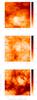 |
Fig. 1 Mean brightness temperature of the CGPS H i emission distribution between the velocity range from: upper panel: +3 to −19 km s-1, middle panel: −20 to −35 km s-1, and lower panel: −41 to −48 km s-1. |
To better analyse the area regarding velocities below −20 km s-1, Fig. 2 shows 12 images covering the velocity range from −53.4 to −24.55 km s-1. Each image shows the mean brightness temperature of three consecutive CGPS velocity channels. Though the H i minimum shown in Fig. 1 (middle and lower panels) is clearly observable in most of the images, a closer look at them shows that the barycentral coordinates of the H i minimum detected at more positive velocities are slightly shifted from those observed at more negative velocities. This is better seen in Fig. 3, where the Galactic coordinates of the H i shell’s barycentre, as a function of the radial velocity, are shown. The barycentric coordinates have been calculated by fitting an ellipse for different radial velocities, whose input points are the maxima of H i emission surrounding the H i voids. The uncertainty in the centroid is typically  . Strikingly enough, the barycentric Galactic longitude of the H i minimum differs by ~1° between −35≤v ≤−25 km s-1 and −50 ≤ v ≤ −40 km s-1. A shift of about 0.3° is also observed in the feature’s centroid at Galactic latitude. Thus, we believe that along the velocity interval −50 ≤ v ≤ −25 km s-1 we are dealing with two different Galactic features and not just with one single structure.
The feature observed at more negative velocities is catalogued as GS 118+01−44 by Suad et al. (2014). This feature has a good morphological correspondence with that found by Fich (1986). From here onwards we concentrate our study on this feature.
3.2. GS 118+01−44
An inspection of Fig. 2 clearly shows the presence of a well-defined local H i minimum in brightness temperature that we identify as GS 118+01−44. This feature is centred at  . To better determine the velocity interval where this structure is seen, an averaged profile has been derived within a
  box centred at
  along the velocity range from −15 to −80 km s-1 (see Fig. 4). There GS 118+01−44 is detected between the peak of emission located at about −35.0 km s-1 and the shoulder detected at about −52.3 km s-1, which corresponds to the H i emission seen at −52.6 km s-1 in the central position of GS 118+01−44 in Fig. 2. On the other hand, the emission observed at −35.0 km s-1 is associated with the emission detected at in the middle panel of Fig. 1. From Fig. 4 it can be inferred that the systemic velocity (v0, where the feature attains its maximum angular extent) of GS 118+01−44 is −44 ± 2 km s-1.
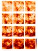 |
Fig. 2 CGPS neutral hydrogen emission in the environs of GS 118+01−44. Each panel shows the mean brightness temperature within three consecutive velocity channels. At the top of each panel the central velocity is indicated. |
The mean brightness temperature distribution in the velocity range from −41.9 to − 47.6 km s-1 is shown in Fig. 5. Since the main physical parameters given for GS 118+01−44 in the catalogue of Suad et al. (2014) were obtained using the Leiden-Argentine-Bonn (LAB) survey Kalberla et al. (2005; FWHM 30′), we now use the CGPS data available for this structure to recalculate them. To this end, an ellipse has been fitted to the H i shell with the classical minimum mean square error (MMSE) technique (Halir & Flusser 1998). Every point used in this fitting corresponds to the local maximum brightness temperature that surrounds the H i minimum. The obtained ellipse is shown superimposed in Fig. 5, where we indicate its centroid  , its major and minor semi-axes
  and
and  , respectively, and the inclination angle (φ) of the semi-major axis with respect to the Galactic plane, φ = 126° ± 4° (measured counterclockwise from the Galactic plane).
According to the systemic velocity of the structure, and taking the non-circular motions present in this region into account (Brand & Blitz 1993), we estimated a distance to the Sun of 3.0 ± 0.6 kpc for GS 118+01−44. At this distance, the major and minor semi-axes are 140 ± 30 and 60 ± 10 pc, respectively, and the effective radius of the structure is  pc.
pc.
To determine the total gaseous mass associated with the supershell, we used MHI = NHIAHI, where NHI is the H i column density,  , v1 = −35.0 km s-1 and v2 = −52.3 km s-1 are the velocity interval, where the structure is detected and Tb the brightness temperature. The parameter AHI is the area of the supershell, AHI = ΩHId2, where ΩHI is the solid angle covered by the structure and d is the distance to the Sun. Adopting solar abundances, we estimated a total gaseous mass of Mt = 1.34 MHI = (4.9 ± 2.2) × 105M⊙.
The dynamic age of the structure is defined as tdyn = Ref/vexp, where vexp is the expansion velocity of the feature (vexp = Δv/ 2, where Δv is the velocity range where the structure is observed). Adopting vexp = 8.7 ± 1.6 km s-1, we obtained tdyn = 10.8 ± 2.6 Myr.
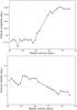 |
Fig. 3 Baricentral coordinates of the two structures observed at different radial velocities. Upper panel: Galactic longitude baricentral coordinates versus radial velocity. Lower panel: Galactic latitude baricentral coordinate versus radial velocity. |
4. CO emission
In this section, we analyse the CO emission distribution looking for molecular clouds possibly related to GS 118+01−44. A CO profile depicting the mean molecular emission originated within a rectangular region of 4.̊2 × 5.̊05 in size and centred at (l,b) = ( 117.̊6, 1.̊4) is shown in the top panel of Fig. 6. As can be seen from this profile, although in this region the bulk of the molecular emission arises from the velocity interval between 5 and –25 km s-1, an additional, smaller peak is detected in the velocity range from about −40 to −53 km s-1. Taking into account the systemic velocity estimated for the H i structure, v0 = −44 km s-1, we infer that this emission may stand a chance of being associated with GS 118+01−44. In the bottom panel of Fig. 6, the H i emission distribution averaged as in Fig. 5 is shown with the CO emission present in the velocity range from −53 to − 40 km s-1 indicated by contours. The presence of several small and disperse CO clouds around GS 118+01−44 can be observed.
It is difficult to determine whether there is a relationship among these small molecular clouds and the H i supershell. Moreover, the origin of these molecular features is not clear. Either they are part of a pre-existing molecular cloud, which was dissociated and fragmented by the action of the massive stars or they were created in the inner parts of the dense H i wall, as proposed by Dawson et al. (2011, 2015).
To characterize these molecular features, we calculated their molecular masses using the relationship N(H2) = XWCO, where N(H2) is the H2 column density, X is the CO-to-H2 conversion factor, X = 1.9 × 1020 cm-2 (K km s-1)-1 (Grenier & Lebrun 1990; Digel et al. 1995), and  is the integrated CO line intensity over the velocity range from − 53 to − 40 km s-1. Then, the molecular mass of each cloud was derived from MH2 [ M⊙ ] = 4.2 × 10⁻²⁰N(H2) d2A, where d is the distance in pc and A is the area in steradians. The estimated mass of the small clouds ranges from around 15 to 1.6 × 10⁴M⊙, and summing all the observed structures, we obtained a total molecular mass of MH2 = (7.4 ± 3.2) × 104M⊙, where the uncertainty arises mainly from the area estimates and the adopted distance. This amount of mass is just the 20% of the H i mass inferred to be present in the shell.
5. Radio continuum
We now study the distribution of the radio continuum emission in the region of GS 118+01−44 using CGPS data at 408 and 1420 MHz. Figure 7 (upper panel) shows the emission at 1420 MHz, with the ellipse delineating the location of GS 118+01−44 superimposed. The presence of several bright and extended regions, already catalogued as H ii regions and SNRs, are evident. According to the WISE Catalog of Galactic H ii regions2 (Anderson et al. 2014), the H ii regions Sh2-165, Sh2-168, Sh2-169, and Sh2-172 have radial velocities in the range from − 42.6 to − 47.9 km s-1, which coincides with the radial velocity interval where GS 118+01−44 is detected. Given the relative location among the mentioned H ii regions and GS 118+01−44 in the plane of the sky and in velocity, we cannot discard the possibility that these structures were related to each other. On the other hand, three SNRs are observed in this area, namely G116.5+1.1, CTB1, and Tycho. The estimated distances of the SNRs shown in Fig. 7 (upper panel) are 1.6 kpc for G116.5+1.1 and CTB 1 (Yar-Uyaniker et al. 2004), and 2.4 kpc for Tycho (Lee et al. 2004). Although Tycho is the nearest to GS 118+01−44, it is located outside the borders of the supershell. Therefore, these SNRs are very likely not associated with GS 118+01−44.
Besides the H ii regions and SNRs, Fig. 7 (upper panel) shows a minimum in the radio continuum emission coincident with the interior part of the H i shell, while diffuse emission is detected around it. To carry out a study of the nature of the diffuse continuum emission, we studied the general distribution of the temperature spectral index. The spectrum of radio continuum radiation is usually described by the temperature spectral index β (Tb ~ ν− β, where Tb is the brightness temperature at the frequency ν). The flux spectral index α is related to β as α = β − 2.
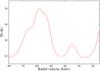 |
Fig. 4 Averaged H i profile in a |
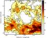 |
Fig. 5 Mean brightness temperature of the H i emission distribution associated with GS 118+01−44 in the velocity range from −41.9 to −47.6 km s-1. Contour levels are at 35 and 55 K. Angular resolution is 2′. |
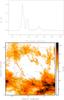 |
Fig. 6 Top panel: mean CO emission within a rectangular area 4.̊2 × 5.̊05 in size, centred at (l,b) = ( 117.̊6, 1.̊4). Bottom panel: mean brightenss temperature of the CGPS H i emission distribution in the velocity range from − 41.9 to − 47.6 km s-1. The contour corresponds to the 1.7 K level of the CO emission integrated in the velocity interval from –53 to –40 km s-1. The ellipse is that fitted for the H i data and the box indicates the area used to obtain the CO profile shown in the top panel. |
To analyse the distribution of the temperature spectral index across the map, an adjustment of the adopted Galactic zero levels of the different survey frequencies, and the overall Galactic background continuum emission have to be subtracted out. To this aim we applied the background filtering method (BGF) developed by Sofue & Reich (1979). A 4° × 4° deg filtering beam was applied to each frequency. The DRAO data at 408 MHz and 1420 MHz were first smoothed by a Gaussian beam to the angular resolution of 6′× 6′. The corresponding final rms of these images are σ1420 = 0.4 K at 1420 MHz and σ408 = 0.03 K at 408 MHz.
The temperature spectral index between two frequencies ν1 (408 MHz) and ν2 (1420 MHz) is calculated pixel wise from
 where we used values for Tb greater than 3σ for both frequencies. The resulting temperature spectral index map is shown in Fig. 7 (lower panel). This map shows a spectrum that is a mixture of synchrotron emission and thermal emission. Flat spectrum areas (β = 2.1), where thermal emission is a significant component, were only found towards the eastern region of GS 118+01−44 between
  and
and  . The values for the non-thermal emission mostly run between 2.3 ≤ β ≤ 2.7 and dominate the remaining parts of the shell. The errors, stemming from the uncertainty in determining the background levels, are of the order of Δ β = 0.1.
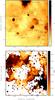 |
Fig. 7 Upper panel: CGPS radio continuum emission at 1420 MHz in the area of GS 118+01−44. The Sharpless H ii regions and SNRs present in the region are labelled. Lower panel: temperature spectral index map. The ellipse delineates the H i supershell location. |
6. Infrared emission
At mid- and far-infrared wavelengths the region occupied by the H i supershell shows a complex morphology, although there is clearly a minimum of IR emission at the centre and some compact enhancement at its borders, i.e. it mimics some of the structure defined by the H i shell. This spatial distribution of the IR emission is detected at wavelengths as short as 12 μm (WISE) and as long as 550 μm (Planck). Figure 8 shows a three-colour image with WISE 12 μm in blue, Planck 550 μm in green, and the CGPS H i emission averaged between − 41.9 and − 47.6 km s-1 in red, with an overlay of the ellipse fitted in the H i data centred at  . The available Herschel data from the HiGAL Survey (Molinari et al. 2010) does not entirely cover the GS 118+01−44 region, as shown in the 160 μm map (see Fig. 9).
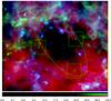 |
Fig. 8 Colour-composite image of the area of GS 118+01−44. Blue shows the emission at 12 μm (W3 WISE band), green represents the emission at 550 μm (Planck), and red shows the mean brightness temperature of the CGPS H i emission distribution between the velocites −41.9 and −47.6 km s-1. The ellipse superimposed is that fitted for the CGPS H i data and the square regions delimit the zones where the fluxes have been calculated. |
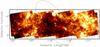 |
Fig. 9 Infrared emission distribution at 160 μm in a partial region of GS 118+01−44. The ellipse superimposed is that fitted for the CGPS H i data. Regions with less infrared emission are shown as dark regions. |
6.1. The dust properties
One of the questions that can be addressed with the mid- and far-infrared continuum data is that of the properties of the dust in the shell, such as its temperature and mass. For this analysis, we followed the standard technique using dust models to match the mid- to far-IR spectral energy distribution (SED); and based on the best fits to constrain the dust properties. We used the recently release DUSTEM (Compiègne et al. 2011) models that use a combination of three dust components, polycyclic aromatic hydrocarbons (PAH), very small (VSG) and big dust grains (BGs), to interpret the emission from dust between ~3 to 1000 μm (see e.g. Li & Draine 2001; Compiègne et al. 2010, 2011). Currently the available version of DUSTEM is missing the necessary database to include the WISE bands in the modelling. This is in part because the Atlas WISE images are not delivered in flux density units (Compiègne, priv. comm.).
Flux densities estimated for regions 1, 2, 3, and 4.
To characterize the dust properties, we selected four regions (1° × 1°) located at the edge of the shell, as indicated in Fig. 8. The integrated flux densities for these regions were estimated by, first, convolving with a 5′ Gaussian beam, to match the lower resolution of the 550 μm Planck image, all the images, i.e. 65, 90, 140, and 160 μm (from AKARI), plus 350 μm (from Planck). And, second, via an On and Off over the shell measurements; this last image was taken at the centre of the supershell and was subtracted from the On value to try to mitigate the effect of the foreground emission contamination, which is expected to be present on most line-of-sight measurements. The estimated flux densities are listed in Table 2.
Figure 10 shows a section of the far-IR SED for region 1 (upper left panel), region 2 (upper right panel), region 3 (lower left panel), and region 4 (lower right panel). On this wavelength range one can find an equilibrium dust temperature set by the thermal balance of the big dust grains and surrounding radiation field. Smaller dust grains are stochastically heated, and therefore, it is meaningless to assign them a dust temperature (see e.g. Draine & Li 2001). For each region, the models provide the interstellar radiation field (ISRF; Mathis et al. 1983) needed for the dust to reach thermal balance, the total mass of dust (D_M), and the temperatures for the three dust components that are assembled at the wavelength range responsible for the infrared radiation, i.e. small carbon (smC), large carbon (laC), and silicates (Si). The parameters derived from the SED fittings are listed in Table 3. In all four regions the ISRF is within a factor 2 of the mean standard value for the interstellar medium and this indicates that the involved radiation fields are not strong. The dust temperature from the carbon grains also reflect this trend with values close to 20 K, very representative of the more diffuse interstellar medium (Boulanger et al. 1996). However, the temperature of the large silicates grains is indeed ~5–6 deg lower in three of the regions, and within the range of values expected for cold molecular gas (see e.g. Flagey et al. 2009) based on far-IR measurements. This mixture of temperatures is unavoidable as we measure the flux densities along the line of sight. The temperatures derived for region 3 are systematically higher by 5–7 deg. Although this could be real, it may reflect some contamination of the measurements by the presence of the Sh2-168 and 169 H ii regions that are found nearby along the line of sight. The small hump or bump in the dotted line at shorter wavelengths (see Fig. 10, lower right panel) indicates that there is enough contribution of VSGs to the SED to correspond to around 10% of the total mass of dust that is still dominated by BGs.
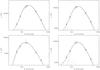 |
Fig. 10 SED of regions number 1 (upper left panel), 2 (upper right panel), 3 (lower left panel), and 4 (lower right panel). Diamonds indicate DUSTEM model prediction and fit. The red error bars denote photometric measurements at 65 μm, 90 μm, 140 μm, and 160 μm (AKARI), 350 μm, and 550 μm (Planck). The solid line shows the VSG+BG model, the dotted line at longer wavelength indicates the BGs, and the dotted line at shorter wavelength indicates the VSGs models. |
7. Origin of GS 118+01−44
In this section, we analyse whether the origin of the supershell can be attributed to the action of stellar winds of massive stars and/or to the subsequent explosion as supernova. Along the narrow Galactic longitude range of about 10° from l ~ 110° to l ~ 120°, at least four OB associations (Cas OB2, Cas OB5, Cep OB4, and Cas OB4) have been catalogued (Garmany & Stencel 1992). All of these but Cep OB4 are located in the Perseus arm, and their heliocentric distances fall in the range from 1.8 to 2.8 kpc. According to their mean Galactic longitude and latitude as derived by Mel’Nik & Dambis (2009), only Cas OB5,  , is located within the ellipse delineating GS 118+01−44. These authors also give a mean heliocentric distance of 2 kpc for Cas OB5, which, bearing in mind the large errors involved in distances of OB associations, could be compatible with the distance derived for GS 118+01−44. The fact that the mean Galactic coordinates of Cas OB5 do not coincide with the centre of GS 118+01−44 could be due to the presence of inhomogeneities of the interstellar medium and/or the possibility that some star members of Cas OB5 could have travelled from their hypothetical central position towards its present location owing to their peculiar spatial motions.
Although the long kinematic timescale of about 11 Myr estimated for GS 118+01−44 suggests that more than one generation of massive stars should be involved and/or that contributions from one or more SN explosion are to be expected, as a first step we carried out energetic analysis to test whether the energy injected by the Cas OB5 stars lying inside GS 118+01−44 could have created the supershell. Those stars are listed in Table 4. Column 1 gives the stars identification, Cols. 2 and 3 their Galactic coordinates, and Col. 4 their spectral types as given by Garmany & Stencel (1992). We estimated the main-sequence (MS) spectral type for each star (Col. 5) based on the evolutionary track models published by Schaller et al. (1992), and adopting the bolometric magnitudes and effective temperatures given by Garmany & Stencel (1992). Column 6 gives an estimate of the star MS lifetime (t(MS)) as derived from the stellar models of Schaller et al. (1992). The values given in this column are a rough estimate as a consequence of the uncertainty in the mass adopted for each star. Columns 7 and 8 give the mass loss rates (Ṁ) and wind velocities (Vw) taken from Lamers & Leitherer (1993) and Leitherer et al. (1992), respectively. Column 9 gives the total wind energy released by each star during its main-sequence phase,  t(MS). Given that BD+61 2554, BD+61 2549, BD+61 2559, LSI+61 112, BD+62 2332, and HD 108 are still in the MS, their values are upper limits. Assuming that these stars belong to Cas OB5, it is evident that the star formation process in the association was not coeval and at least these six stars may have been formed later.
On the other hand, taking the total gaseous and molecular mass of GS 118+01−44 derived in previous sections into account, the kinetic energy stored in the shell can be calculated as  erg. From the last column of Table 4, we infer that the total wind energy injected by the listed stars is Ew ~ 4.7 × 1050 erg, which would only be sufficient to create GS 118+01−44 in the case in which the energy conversion efficiency from the wind energy into mechanical energy, ϵ = Ekin/Ew, were higher than ~85%. This efficiency is too high even if the theoretical energy conserving model, which yields ϵ = 0.2, were applicable (Weaver et al. 1977).
Therefore, an additional energy source seems to be needed to explain the supershell’s origin. If the origin of GS 118+01−44 is indeed the action of many massive stars, for the sake of illustration we can estimate how many of them would have been needed to create it. Taking ϵ = 0.2 and adopting mean stellar wind parameters for O-type stars (Mokiem et al. 2007) we find, for instance, that either four O6, or seven O7, or 83 B0 type stars are needed to create the structure.
However, since SNe are believed to play a predominant role in shaping the large-scale structure of the ISM (e.g. Hennebelle & Iffrig 2014) and the fact that the region under study involved several OB associations and large H i shells, we cannot discard the possibility that at least one supernova explosion had already taken place in the region. To evaluate this possibility, we can make some rough estimations.
According to Cioffi et al. (1988) the maximum observable radius of an SNR before it merges with the ISM is given by
 where E0 is the explosion energy in units of 1051 erg, n the mean ambient particle density in cm-3, and Z the metallicity normalized to the solar value. The ambient density strongly depends on the Galactocentric distance (R) and the distance z above the disk. To estimate the ambient density, we made use of H i distribution model for the outer Milky Way given by Kalberla & Dedes (2008), which yields, for 7 ≤ R ≤ 35 kpc, the following radial distribution:
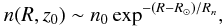 where n0 = 0.9 cm-3, R⊙ = 8.5 kpc, and Rn = 3.15 kpc is the radial scale length. Assuming for GS 118+01−44 a Galactocentric distance of R = 10.3 kpc, we obtain n0 ~ 0.5 cm-3. Thus, for a solar metallicity and E0 = 1, we obtain Rmerge ~ 66 pc, while for E0 = 2, Rmerge turns out to be about 82 pc. If we assume a lower metallicity value, Z = 0.1, we obtain Rmerge ~ 74 and Rmerge ~ 93 pc, for E0 = 1 and E0 = 2, respectively. Thus, bearing in mind all the approximations used in these estimates, we believe that a scenario in which several OB stars acted through their winds together with one or two SNe is plausible to explain the origin of GS 118+01−44.
Parameters derived from the SEDs.
Cas OB5 stars lying inside GS 118+01−44.
8. Star formation
To analyse whether star formation is still taking place in the region, we attempt to identify young stellar object candidates (cYSOs) located in projection onto the molecular gas possibly related to GS 118+01−44. To this end, we made used of the IRAS Point Source Catalogue (Beichman et al. 1988), the MSX Infrared Point Source Catalogue (Egan et al. 2003), and the WISE All-Sky Source Catalog (Wright et al. 2010). Within a circular area of 3 deg radius, centred at (l,b) = (117.̊8, 1.̊1), a total of 605 IRAS, 32 MSX, and 91191 WISE sources were found. From the MSX catalogue, we only considered those sources with acceptable flux quality (q ≥ 2) in the four bands, while we selected only the sources with a photometric uncertainty ≤0.2 mag and S/N ≥ 7 in all four bands for the WISE catalogue.
To identify the cYSOs among all the listed infrared sources, we applied colour criteria that are widely used to this end. In the case of the IRAS sources, we followed the Junkes et al. (1992) colour criteria and select, among the 605 sources listed, 32 cYSOs. As for the MSX sources, we applied the Lumsden et al. (2002) criteria, and found six massive young stellar objects (MYSO) candidates. To classify the WISE sources, we adopted the classification scheme described in Koenig et al. (2012), where the first step consists in removing various non-stellar sources, such as PAH-emitting galaxies, broad-line active galactic nuclei (AGNs), resolved knots of shock emission, and resolved structured PAH-emission features from the listed sources. In this case, we removed a total of 46136 sources. Then, applying the colour criteria given by Koenig et al. (2012) to the remaining sample of 45055 sources, we identified 148 Class I (sources where the IR emission arises mainly from a dense infalling envelope) and 385 Class II (sources where the IR emission is dominated by the presence of an optically thick circumstellar disk) cYSOs.
Bearing in mind that star formation takes place in molecular clouds, as an additional constraint we selected, from all the cYSOs found, only those lying in projection onto molecular gas observed in the velocity range from –53 to –40 km s-1 (see Fig. 6, upper panel). Finally, after applying this constraint, the list of cYSOs contains 11 IRAS sources, 2 MYSOs, and 92 WISE sources, 32 Class I, and 60 Class II.
Figure 11 shows the integrated CO emission distribution in the velocity range considered with the final list of cYSOs overlaid. Different symbols indicates different classes of sources. It is important to mention that in the direction of 61 of the total cYSOs, CO emission is only observed in the velocity range from –53 to –40 km s-1 (they are indicated in red in Fig. 11), while in the direction of the rest, 31 sources the CO profile presents more than one component (these cYSOs are in blue in Fig. 11). From Fig. 11, it is clear that the region is still undergoing star formation.
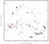 |
Fig. 11 Integrated CO emission distribution in the velocity range from –53 to –40 km s-1. Contour level is at 2.0 K. The location of the cYSOs are indicated with different symbols according to the catalogue where they were found: MSX: circles; IRAS: asteriscs; WISE: plus signs correspond to Class I objects and crosses correspond to Class II. Red and blue indicate objects in which direction there is just one CO component or more than one, respectively. |
9. Conclusions
In this work we have studied in detail the structure labelled GS 118+01−44 in the supershell candidates catalogue of Suad et al. (2014). This feature is a well-defined H i supershell centred at (l,b) = (117.̊7, 1.̊4), with an effective radius of Ref = 94 ± 15 pc, and a total gaseous and molecular mass of Mt = (4.9 ± 2.2) × 105M⊙ and MH2 = (7.4 ± 3.2) × 104M⊙, respectively.
Diffuse radio continuum emission is detected around the supershell. A study of the temperature spectral index distribution reveals that thermal emission is only found in a small region, located towards the eastern boundary of GS 118+01−44, while non-thermal emission dominates the remaining parts. We have also compared the morphology of the H i supershell with that observed in the mid- and far-IR and conclude that they are quite similar, in particular, in the range of H i velocities from −41.9 to −47.6 km s-1, suggesting that dust components coexist with the H i gas. Based on this good morphological coincidence, we used far-IR measurements to determine the dust temperature of four regions located around the supershell. For three of these regions, we found a mean dust temperature of 19.3 K, as traced by the Big Grains, not far from that expected in molecular gas. The fourth region is a bit warmer and closer in temperature to what is expected for the diffuse interstellar medium.
We conclude, based on an energetic analysis, that the origin of GS 118+01−44 could be attributed to the mechanical energy injected by the winds of the star members of Cas OB5 observed projected towards the inner part of the shell in combination with another energy source, such as the stellar winds of other massive stars and/or one or two SN explosion. This result is in agreement with the predominance of non-thermal emission found around GS 118+01−44.
We have also analysed the possible association of several H ii regions and three SNRs that are seen superimposed on the line-of-sight radio continuum maps and conclude that, based on their known distances or radial velocities, none of the SNRs and some of the H ii regions are physically related to the H i supershell. On the other hand, four of the H ii regions may be at the same distance of GS 118+01−44. The fact that these four H ii regions are projected onto the supershell borders leads us to the conclusion that they may have been created as a consequence of the action of a strong shock produced by the expansion of GS 118+01−44 into the surrounding molecular gas.
In the region under study there are several small CO clouds observed around the supershell that could be either the debris of the original CO cloud out of which Cas OB5 was created or they were created in the dense walls of GS 118+01−44.
All the evidence found in this mutliwavelength study support the idea that GS 118+01−44 is actually a physical structure with dense and molecular gas. On the other hand, the presence of several cYSOs projected onto the molecular clouds and four H ii regions detected onto the supershell allow us to conclude that the area is still an active star-forming region.
Acknowledgments
We thank the referee for her/his careful reading and comments on the manuscript that has helped us to improve its content and presentation. The CGPS is a Canadian Project with international partners and is supported by grants from NSERC. Data from the CGPS are publicly available through the facilities of the Canadian Astronomy Data Centre (http://cadc.hia.nrc.ca) operated by the Herzberg Institute of Astrophysics, NRC. This project was partially financed by the Consejo Nacional de Investigaciones Científicas y Técnicas (CONICET) of Argentina under project PIP 01299, Agencia PICT 00902, and UNLP G091. L.A. Suad is a post-doctoral fellow of CONICET, Argentina. S. Cichowolski and E.M. Arnal are members of the Carrera del Investigador Científico of CONICET, Argentina. J.C. Testori is member of the Carrera del Personal de Apoyo, CONICET, Argentina.
References
- Anderson, L. D., Bania, T. M., Balser, D. S., et al. 2014, ApJS, 212, 1 [NASA ADS] [CrossRef] [Google Scholar]
- Arnal, E. M., & Corti, M. 2007, A&A, 476, 255 [NASA ADS] [CrossRef] [EDP Sciences] [Google Scholar]
- Bagetakos, I., Brinks, E., Walter, F., et al. 2011, AJ, 141, 23 [NASA ADS] [CrossRef] [Google Scholar]
- Beichman, C. A., Neugebauer, G., Habing, H. J., Clegg, P. E., & Chester, T. J., 1988, Infrared astronomical satellite (IRAS) catalogs and atlases, Vol. 1: Explanatory suppl., 1 [Google Scholar]
- Boulanger, F., Abergel, A., Bernard, J.-P., et al. 1996, A&A, 312, 256 [NASA ADS] [Google Scholar]
- Brand, J., & Blitz, L. 1993, A&A, 275, 67 [NASA ADS] [Google Scholar]
- Cichowolski, S., Romero, G. A., Ortega, M. E., Cappa, C. E., & Vasquez, J. 2009, MNRAS, 394, 900 [NASA ADS] [CrossRef] [Google Scholar]
- Cichowolski, S., Pineault, S., Gamen, R., et al. 2014, MNRAS, 438, 1089 [NASA ADS] [CrossRef] [Google Scholar]
- Cioffi, D. F., McKee, C. F., & Bertschinger, E. 1988, ApJ, 334, 252 [NASA ADS] [CrossRef] [Google Scholar]
- Compiègne, M., Flagey, N., Noriega-Crespo, A., et al. 2010, ApJ, 724, L44 [NASA ADS] [CrossRef] [Google Scholar]
- Compiègne, M., Verstraete, L., Jones, A., et al. 2011, A&A, 525, A103 [NASA ADS] [CrossRef] [EDP Sciences] [Google Scholar]
- Dawson, J. R., McClure-Griffiths, N. M., Dickey, J. M., & Fukui, Y. 2011, ApJ, 741, 85 [NASA ADS] [CrossRef] [Google Scholar]
- Dawson, J. R., Ntormousi, E., Fukui, Y., Hayakawa, T., & Fierlinger, K. 2015, ApJ, 799, 64 [NASA ADS] [CrossRef] [Google Scholar]
- Digel, S. W., Hunter, S. D., & Mukherjee, R. 1995, ApJ, 441, 270 [NASA ADS] [CrossRef] [Google Scholar]
- Draine, B. T., & Li, A. 2001, ApJ, 551, 807 [NASA ADS] [CrossRef] [Google Scholar]
- Egan, M. P., Price, S. D., Kraemer, K. E., et al. 2003, VizieR Online Data Catalog: V/114 [Google Scholar]
- Ehlerová, S., & Palouš, J. 2005, A&A, 437, 101 [NASA ADS] [CrossRef] [EDP Sciences] [Google Scholar]
- Ehlerová, S., & Palouš, J. 2013, A&A, 550, A23 [NASA ADS] [CrossRef] [EDP Sciences] [Google Scholar]
- Fich, M. 1986, ApJ, 303, 465 [NASA ADS] [CrossRef] [Google Scholar]
- Flagey, N., Noriega-Crespo, A., Boulanger, F., et al. 2009, ApJ, 701, 1450 [NASA ADS] [CrossRef] [Google Scholar]
- Garmany, C. D., & Stencel, R. E. 1992, A&AS, 94, 211 [NASA ADS] [Google Scholar]
- Grenier, I. A., & Lebrun, F. 1990, ApJ, 360, 129 [NASA ADS] [CrossRef] [Google Scholar]
- Halir, R., & Flusser, J. 1998, The Sixth International Conference in Central Europe on Computer Graphics and Visualization, 125 [Google Scholar]
- Hartmann, D., & Burton, W. B. 1997, Atlas of Galactic Neutral Hydrogen (Cambridge, UK: Cambridge University Press) [Google Scholar]
- Heiles, C. 1979, ApJ, 229, 533 [NASA ADS] [CrossRef] [Google Scholar]
- Hennebelle, P., & Iffrig, O. 2014, A&A, 570, A81 [NASA ADS] [CrossRef] [EDP Sciences] [Google Scholar]
- Heyer, M. H., Brunt, C., Snell, R. L., et al. 1998, ApJS, 115, 241 [NASA ADS] [CrossRef] [Google Scholar]
- Junkes, N., Fürst, E., & Reich, W. 1992, A&A, 261, 289 [NASA ADS] [Google Scholar]
- Kalberla, P. M. W., & Dedes, L. 2008, A&A, 487, 951 [NASA ADS] [CrossRef] [EDP Sciences] [Google Scholar]
- Kalberla, P. M. W., Burton, W. B., Hartmann, D., et al. 2005, A&A, 440, 775 [NASA ADS] [CrossRef] [EDP Sciences] [Google Scholar]
- Koenig, X. P., Leisawitz, D. T., Benford, D. J., et al. 2012, ApJ, 744, 130 [NASA ADS] [CrossRef] [Google Scholar]
- Lamers, H. J. G. L. M., & Leitherer, C. 1993, ApJ, 412, 771 [NASA ADS] [CrossRef] [Google Scholar]
- Landecker, T. L., Dewdney, P. E., Burgess, T. A., et al. 2000, A&AS, 145, 509 [NASA ADS] [CrossRef] [EDP Sciences] [Google Scholar]
- Lee, J.-J., Koo, B.-C., & Tatematsu, K. 2004, ApJ, 605, L113 [NASA ADS] [CrossRef] [Google Scholar]
- Leitherer, C., Robert, C., & Drissen, L. 1992, ApJ, 401, 596 [NASA ADS] [CrossRef] [Google Scholar]
- Li, A., & Draine, B. T. 2001, ApJ, 554, 778 [Google Scholar]
- Lumsden, S. L., Hoare, M. G., Oudmaijer, R. D., & Richards, D. 2002, MNRAS, 336, 621 [NASA ADS] [CrossRef] [Google Scholar]
- Martins, F., Escolano, C., Wade, G. A., et al. 2012, A&A, 538, A29 [NASA ADS] [CrossRef] [EDP Sciences] [Google Scholar]
- Mathis, J. S., Mezger, P. G., & Panagia, N. 1983, A&A, 128, 212 [NASA ADS] [Google Scholar]
- McClure-Griffiths, N. M., Dickey, J. M., Gaensler, B. M., & Green, A. J. 2002, ApJ, 578, 176 [NASA ADS] [CrossRef] [Google Scholar]
- Mel’Nik, A. M., & Dambis, A. K. 2009, MNRAS, 400, 518 [NASA ADS] [CrossRef] [Google Scholar]
- Mokiem, M. R., de Koter, A., Vink, J. S., et al. 2007, A&A, 473, 603 [NASA ADS] [CrossRef] [EDP Sciences] [Google Scholar]
- Molinari, S., Swinyard, B., Bally, J., et al. 2010, A&A, 518, L100 [NASA ADS] [CrossRef] [EDP Sciences] [Google Scholar]
- Moór, A., & Kiss, C. 2003, Communications of the Konkoly Observatory Hungary, 103, 149 [NASA ADS] [Google Scholar]
- Planck Collaboration I. 2015, A&A, submitted [arXiv:1502.01582] [Google Scholar]
- Schaller, G., Schaerer, D., Meynet, G., & Maeder, A. 1992, A&AS, 96, 269 [Google Scholar]
- Sofue, Y., & Reich, W. 1979, A&AS, 38, 251 [NASA ADS] [Google Scholar]
- Suad, L. A., Cichowolski, S., Arnal, E. M., & Testori, J. C. 2012, A&A, 538, A60 [NASA ADS] [CrossRef] [EDP Sciences] [Google Scholar]
- Suad, L. A., Caiafa, C. F., Arnal, E. M., & Cichowolski, S. 2014, A&A, 564, A116 [NASA ADS] [CrossRef] [EDP Sciences] [Google Scholar]
- Takita, S., Doi, Y., Ootsubo, T., et al. 2015, PASJ, 67, 51 [NASA ADS] [CrossRef] [Google Scholar]
- Taylor, A. R., Gibson, S. J., Peracaula, M., et al. 2003, AJ, 125, 3145 [NASA ADS] [CrossRef] [Google Scholar]
- Weaver, H., & Williams, D. R. W. 1973, A&AS, 8, 1 [NASA ADS] [Google Scholar]
- Weaver, R., McCray, R., Castor, J., Shapiro, P., & Moore, R. 1977, ApJ, 218, 377 [NASA ADS] [CrossRef] [Google Scholar]
- Wright, E. L., Eisenhardt, P. R. M., Mainzer, A. K., et al. 2010, AJ, 140, 1868 [NASA ADS] [CrossRef] [Google Scholar]
- Yar-Uyaniker, A., Uyaniker, B., & Kothes, R. 2004, ApJ, 616, 247 [NASA ADS] [CrossRef] [Google Scholar]
All Tables
All Figures
|
Fig. 1 Mean brightness temperature of the CGPS H i emission distribution between the velocity range from: upper panel: +3 to −19 km s-1, middle panel: −20 to −35 km s-1, and lower panel: −41 to −48 km s-1. |
| In the text | |
|
Fig. 2 CGPS neutral hydrogen emission in the environs of GS 118+01−44. Each panel shows the mean brightness temperature within three consecutive velocity channels. At the top of each panel the central velocity is indicated. |
| In the text | |
|
Fig. 3 Baricentral coordinates of the two structures observed at different radial velocities. Upper panel: Galactic longitude baricentral coordinates versus radial velocity. Lower panel: Galactic latitude baricentral coordinate versus radial velocity. |
| In the text | |
|
Fig. 4 Averaged H i profile in a |
| In the text | |
|
Fig. 5 Mean brightness temperature of the H i emission distribution associated with GS 118+01−44 in the velocity range from −41.9 to −47.6 km s-1. Contour levels are at 35 and 55 K. Angular resolution is 2′. |
| In the text | |
|
Fig. 6 Top panel: mean CO emission within a rectangular area 4.̊2 × 5.̊05 in size, centred at (l,b) = ( 117.̊6, 1.̊4). Bottom panel: mean brightenss temperature of the CGPS H i emission distribution in the velocity range from − 41.9 to − 47.6 km s-1. The contour corresponds to the 1.7 K level of the CO emission integrated in the velocity interval from –53 to –40 km s-1. The ellipse is that fitted for the H i data and the box indicates the area used to obtain the CO profile shown in the top panel. |
| In the text | |
|
Fig. 7 Upper panel: CGPS radio continuum emission at 1420 MHz in the area of GS 118+01−44. The Sharpless H ii regions and SNRs present in the region are labelled. Lower panel: temperature spectral index map. The ellipse delineates the H i supershell location. |
| In the text | |
|
Fig. 8 Colour-composite image of the area of GS 118+01−44. Blue shows the emission at 12 μm (W3 WISE band), green represents the emission at 550 μm (Planck), and red shows the mean brightness temperature of the CGPS H i emission distribution between the velocites −41.9 and −47.6 km s-1. The ellipse superimposed is that fitted for the CGPS H i data and the square regions delimit the zones where the fluxes have been calculated. |
| In the text | |
|
Fig. 9 Infrared emission distribution at 160 μm in a partial region of GS 118+01−44. The ellipse superimposed is that fitted for the CGPS H i data. Regions with less infrared emission are shown as dark regions. |
| In the text | |
|
Fig. 10 SED of regions number 1 (upper left panel), 2 (upper right panel), 3 (lower left panel), and 4 (lower right panel). Diamonds indicate DUSTEM model prediction and fit. The red error bars denote photometric measurements at 65 μm, 90 μm, 140 μm, and 160 μm (AKARI), 350 μm, and 550 μm (Planck). The solid line shows the VSG+BG model, the dotted line at longer wavelength indicates the BGs, and the dotted line at shorter wavelength indicates the VSGs models. |
| In the text | |
|
Fig. 11 Integrated CO emission distribution in the velocity range from –53 to –40 km s-1. Contour level is at 2.0 K. The location of the cYSOs are indicated with different symbols according to the catalogue where they were found: MSX: circles; IRAS: asteriscs; WISE: plus signs correspond to Class I objects and crosses correspond to Class II. Red and blue indicate objects in which direction there is just one CO component or more than one, respectively. |
| In the text | |
Current usage metrics show cumulative count of Article Views (full-text article views including HTML views, PDF and ePub downloads, according to the available data) and Abstracts Views on Vision4Press platform.
Data correspond to usage on the plateform after 2015. The current usage metrics is available 48-96 hours after online publication and is updated daily on week days.
Initial download of the metrics may take a while.