| Issue |
A&A
Volume 584, December 2015
|
|
|---|---|---|
| Article Number | A103 | |
| Number of page(s) | 22 | |
| Section | Stellar structure and evolution | |
| DOI | https://doi.org/10.1051/0004-6361/201526642 | |
| Published online | 27 November 2015 | |
Unified equation of state for neutron stars on a microscopic basis
1
Departament d’Estructura i Constituents de la Matèria and Institut
de Ciències del Cosmos (ICC), Facultat de Física, Universitat de
Barcelona, Diagonal
645, 08028
Barcelona,
Spain
2
Department of Sciences, Amrita Vishwa Vidyapeetham Ettimadai,
641112
Coimbatore,
India
3
INFN Sezione di Catania, via Santa Sofia 64,
95123
Catania,
Italy
e-mail:
This email address is being protected from spambots. You need JavaScript enabled to view it.
Received: 30 May 2015
Accepted: 11 September 2015
Abstract
We derive a new equation of state (EoS) for neutron stars (NS) from the outer crust to the core based on modern microscopic calculations using the Argonne v18 potential plus three-body forces computed with the Urbana model. To deal with the inhomogeneous structures of matter in the NS crust, we use a recent nuclear energy density functional that is directly based on the same microscopic calculations, and which is able to reproduce the ground-state properties of nuclei along the periodic table. The EoS of the outer crust requires the masses of neutron-rich nuclei, which are obtained through Hartree-Fock-Bogoliubov calculations with the new functional when they are unknown experimentally. To compute the inner crust, Thomas-Fermi calculations in Wigner-Seitz cells are performed with the same functional. Existence of nuclear pasta is predicted in a range of average baryon densities between ≃0.067 fm-3 and ≃0.0825 fm-3, where the transition to the core takes place. The NS core is computed from the new nuclear EoS assuming non-exotic constituents (core of npeμ matter). In each region of the star, we discuss the comparison of the new EoS with previous EoSs for the complete NS structure, widely used in astrophysical calculations. The new microscopically derived EoS fulfills at the same time a NS maximum mass of 2 M⊙ with a radius of 10 km, and a 1.5 M⊙ NS with a radius of 11.6 km.
Key words: dense matter / equation of state / stars: neutron
© ESO, 2015
1. Introduction
Neutron stars (NS) harbor unique conditions and phenomena that challenge the physical theories of matter. Beneath a thin stellar atmosphere, a NS interior consists of three main regions, namely, an outer crust, an inner crust, and a core, each one featuring a different physics (Shapiro & Teukolsky 1983; Haensel et al. 2006; Chamel & Haensel 2008). The core is the internal region at densities larger than 1.5 × 10¹⁴ g/cm3, where matter forms a homogeneous liquid composed of neutrons plus a certain fraction of protons, electrons, and muons that maintain the system in β equilibrium. Deep in the core, at still higher densities, strange baryons and even deconfined quarks may appear (Shapiro & Teukolsky 1983; Haensel et al. 2006). Moving from the core to the exterior, density and pressure decrease. When the density becomes lower than approximately 1.5 × 10¹⁴ g/cm3, matter inhomogeneities set in. The positive charges concentrate in individual clusters of charge Z and form a solid lattice to minimize the Coulomb repulsion among them. The lattice is embedded in a gas of free neutrons and a background of electrons such that the whole system is charge neutral. This region of the star is called the inner crust, where the nuclear structures may adopt non-spherical shapes (generically referred to as nuclear pasta) in order to minimize their energy (Baym et al. 1971a; Ravenhall et al. 1983; Lorenz et al. 1993; Oyamatsu 1993). At lower densities, neutrons are finally confined within the nuclear clusters and matter is made of a lattice of neutron-rich nuclei permeated by a degenerate electron gas. This region is known as the outer crust (Baym et al. 1971b) and extends, from inside to outside, from a neutron drip density of about 4 × 10¹¹ g/cm3 to a density of about 104 g/cm3. Most of the mass and size of a NS are accounted for by its core. Although the crust is only a small fraction of the star mass and radius, the crust plays an important role in various observed astrophysical phenomena such as pulsar glitches, quasiperiodic oscillations in soft gamma-ray repeaters (SGR), and thermal relaxation in soft X-ray transients (SXT; Haensel et al. 2006; Chamel & Haensel 2008; Piro 2005; Strohmayer & Watts 2006; Steiner & Watts 2009; Sotani et al. 2012; Newton et al. 2013; Piekarewicz et al. 2014), which depend on the departure of the star from the picture of a homogeneous fluid. Recent studies suggest that the existence of nuclear pasta layers in the NS crust may limit the rotational speed of pulsars and may be a possible origin of the lack of X-ray pulsars with long spin periods (Pons et al. 2013; Horowitz et al. 2015).
The equation of state (EoS) of neutron-rich matter is a basic input needed to compute most properties of NSs. A large body of experimental data on nuclei, heavy ion collisions, and astrophysical observations has been gathered and used along the years to constrain the nuclear EoS and to understand the structure and properties of NS. Unfortunately, a direct link of measurements and observations with the underlying EoS is very difficult and a proper interpretation of the data necessarily needs some theoretical inputs. To reduce the uncertainty on these types of analyses, it is helpful to develop a microscopic theory of nuclear matter based on a sound many-body scheme and well-controlled basic interactions among nucleons. To this end, it is of particular relevance to have a unified theory able to describe on a microscopic level the complete structure of NS from the outer crust to the core.
There are just a few EoSs devised and used to describe the whole NS within a unified framework. It is usually assumed that the NS crust has the structure of a regular lattice that is treated in the Wigner-Seitz (WS) approximation. A partially phenomenological approach was developed by Lattimer & Swesty (1991; LS). The inner crust was computed using the compressible liquid drop model (CLDM) introduced by Baym, Bethe, and Pethick (Baym et al. 1971a) to take into account the effect of the dripped neutrons. In the LS model the EoS is derived from a Skyrme nuclear effective force. There are different versions of this EoS (Lattimer & Swesty 1991; Lattimer 2015), each one having a different incompressibility. Another EoS was developed by Shen et al. (Shen et al. 1998b,a; Sumiyoshi 2015) based on a nuclear relativistic mean field (RMF) model. The crust was described in the Thomas-Fermi (TF) scheme using the variational method with trial profiles for the nucleon densities. The LS and Shen EoSs are widely used in astrophysical calculations for both neutron stars and supernova simulations due to their numerical simplicity and the large range of tabulated densities and temperatures.
Douchin & Haensel (2001; DH) formulated a unified EoS for NS on the basis of the SLy4 Skyrme nuclear effective force (Chabanat et al. 1998), where some parameters of the Skyrme interaction were adjusted to reproduce the Wiringa et al. calculation of neutron matter (Wiringa et al. 1988) above saturation density. Hence, the DH EoS contains certain microscopic input. In the DH model the inner crust was treated in the CLDM approach. More recently, unified EoSs for NS have been derived by the Brussels-Montreal group (Chamel et al. 2011; Pearson et al. 2012; Fantina et al. 2013; Potekhin et al. 2013). They are based on the BSk family of Skyrme nuclear effective forces (Goriely et al. 2010). Each force is fitted to the known masses of nuclei and adjusted among other constraints to reproduce a different microscopic EoS of neutron matter with different stiffness at high density. The inner crust is treated in the extended Thomas-Fermi approach with trial nucleon density profiles including perturbatively shell corrections for protons via the Strutinsky integral method. Analytical fits of these neutron-star EoSs have been constructed in order to facilitate their inclusion in astrophysical simulations (Potekhin et al. 2013). Quantal Hartree calculations for the NS crust have been systematically performed by (Shen et al. 2011b,a). This approach uses a virial expansion at low density and a RMF effective interaction at intermediate and high densities, and the EoS of the whole NS has been tabulated for different RMF parameter sets. Also recently, a complete EoS for supernova matter has been developed within the statistical model (Hempel & Schaffner-Bielich 2010). We shall adopt here the EoS of the BSk21 model (Chamel et al. 2011; Pearson et al. 2012; Fantina et al. 2013; Potekhin et al. 2013; Goriely et al. 2010) as a representative example of contemporary EoS for the complete NS structure, and a comparison with the other EoSs of the BSk family (Chamel et al. 2011; Pearson et al. 2012; Fantina et al. 2013; Potekhin et al. 2013) and the RMF family (Shen et al. 2011b,a) shall be left for future study.
Our aim in this paper is to obtain a unified EoS for neutron stars based on a microscopic many-body theory. The nuclear EoS of the model is derived in the Brueckner-Hartree-Fock (BHF) approach from the bare nucleon-nucleon (NN) interaction in free space (Argonne v18 potential, Wiringa et al. 1995) with inclusion of three-body forces (TBF) among nucleons. In the current state of the art of the Brueckner approach, the TBFs are reduced to a density-dependent two-body force by averaging over the third nucleon in the medium (Baldo et al. 1997). We employ TBFs based on the Urbana model, consisting of an attractive term from two-pion exchange and a repulsive phenomenological central term, to reproduce the saturation point (Schiavilla et al. 1986; Baldo et al. 1997, 2012; Taranto et al. 2013). The corresponding nuclear EoS for symmetric and asymmetric nuclear matter fulfills several requirements imposed both by heavy ion collisions and astrophysical observations (Taranto et al. 2013).
Recently the connection between two-body and three-body forces within the meson-nucleon theory of the nuclear interaction has been extensively discussed and developed in (Grangé et al. 1989; Zuo et al. 2002; Li & Schulze 2008; Li et al. 2008). At present the theoretical status of microscopically derived TBFs is still incipient, however a tentative approach has been proposed using the same meson-exchange parameters as the underlying NN potential. Results have been obtained with the Argonne v18, the Bonn B, and the Nijmegen 93 potentials (Li & Schulze 2008; Li et al. 2008). More recently the chiral expansion theory to the nucleon interaction has been extensively developed (Weinberg 1968, 1990, 1991, 1992; Entem & Machleidt 2003; Valderrama & Phillips 2015; Leutwyler 1994; Epelbaum et al. 2009; Otsuka et al. 2010; Holt et al. 2013; Hebeler et al. 2011; Drischler et al. 2014; Hebeler & Schwenk 2010; Carbone et al. 2013; Ekström et al. 2013; Coraggio et al. 2014). This approach is based on a deeper level of the strong interaction theory, where the QCD chiral symmetry is explicitly exploited in a low-momentum expansion of the multi-nucleon interaction processes. In this approach multi-nucleon interactions arise naturally and a hierarchy of the different orders can be established. Despite some ambiguity in the parametrization of the force (Ekström et al. 2013) and some difficulty in the treatment of many-body systems (Laehde et al. 2013), the method has marked a great progress in the microscopic theory of nuclear systems. Indeed it turns out (Coraggio et al. 2014; Ekström et al. 2015) that within this class of interactions a compatible treatment of few-nucleon systems and nuclear matter is possible. However, this class of NN and TBF (or multi-body) interactions is devised on the basis of a low-momentum expansion, where the momentum cut-off is fixed essentially by the mass of the ρ-meson. As such they cannot be used at density well above saturation, where we are also going to test the proposed EoS. In any case, the strength of TBFs is model dependent. In particular, the role of TBFs appears to be marginal in the quark-meson model of the NN interaction (Baldo & Fukukawa 2014).
A many-body calculation of the inhomogeneous structures of a NS crust is currently out of reach at the level of the BHF approach that we can apply for the homogeneous matter of the core. In an attempt to maximize the use of the same microscopic theory for the description of the complete stellar structure, we employ in the crust calculations the recently developed BCPM (Barcelona-Catania-Paris-Madrid) nuclear energy density functional (Baldo et al. 2008b, 2010, 2013). The BCPM functional has been obtained from the ab initio BHF calculations in nuclear matter within an approximation inspired by the Kohn-Sham formulation of density functional theory (Kohn & Sham 1965). Instead of starting from a certain effective interaction, the BCPM functional is built up with a bulk part obtained directly from the BHF results in symmetric and neutron matter via the local density approximation. It is supplemented by a phenomenological surface part, which is absent in nuclear matter, together with the Coulomb, spin-orbit, and pairing contributions. This energy density functional constructed upon the BHF calculations has a reduced set of four adjustable parameters in total and describes the ground-state properties of finite nuclei similarly successfully as the Skyrme and Gogny forces (Baldo et al. 2008b, 2010, 2013).
We model the NS crust in the WS approximation. To compute the outer crust, we take the masses of neutron-rich nuclei from experiment if they are measured, and perform deformed Hartree-Fock-Bogoliubov (HFB) calculations with the BCPM energy density functional when the masses are unknown. To describe the inner crust, we perform self-consistent Thomas-Fermi calculations with the BCPM functional in different periodic configurations (spheres, cylinders, slabs, cylindrical holes, and spherical bubbles). In this calculation of the inner crust, by construction of the BCPM functional, the low-density neutron gas and the bulk matter of the high-density nuclear structures are not only consistent with each other, but they both are given by the microscopic BHF calculation. We find that nuclear pasta shapes are the energetically most favourable configurations between a density of ≃ 0.067 fm-3 (or 1.13 × 10¹⁴ g/cm3) and the transition to the core, though the energy differences with the spherical solution are small. The NS core is assumed to be composed of npeμ matter. We compute the EoS of the core using the nuclear EoS from the BHF calculations. In the past years, the BHF approach has been extended in order to include the hyperon degrees of freedom (Baldo et al. 1998, 2000a), which play an important role in the study of neutron-star matter. However, in this work we are mainly interested on the properties of the nucleonic EoS, and therefore we do not consider cores with hyperons or other exotic components. In each region of the star we critically compare the new NS EoS with the results from various semi-microscopic approaches mentioned above, where the crust and the core were calculated within the same theoretical scheme. Lastly, we compute the mass-radius relation of neutron stars using the unified EoS for the crust and core that has been derived from the microscopic BHF calculations in nuclear matter. The predicted maximum mass and radii are compatible with the recent astrophysical observations and analyses. We reported some preliminary results about the new EoS recently in (Baldo et al. 2014).
In Sect. 2 we summarize the microscopic nuclear input to our calculations and the derivation of the BCPM energy density functional for nuclei. We devote Sect. 3 to the calculations of the outer crust. In Sect. 4 we introduce the Thomas-Fermi formalism for the inner crust with the BCPM functional, and in Sect. 5 we discuss the results in the inner crust, including the pasta shapes. In Sect. 6 we describe the calculation of the EoS in the core and obtain the mass-radius relation of neutron stars. We conclude with a summary and outlook in Sect. 7.
2. Microscopic input and energy density functional for nuclei
As the microscopic BHF EoS of nuclear matter underlies our formulation, we start by summarizing how the EoS of nuclear matter is obtained in the BHF method and how it has been used to construct a suitable energy density functional for the description of finite nuclei.
The nuclear EoS of the model is derived in the framework of the Brueckner-Bethe-Goldstone theory, which is based on a linked cluster expansion of the energy per nucleon of nuclear matter (see Baldo 1999, Chap. 1, and references therein). The basic ingredient in this many-body approach is the Brueckner reaction matrix G, which is the solution of the Bethe-Goldstone equation ![Mathematical equation: \begin{equation} G[\rtheo;\omega] = v + \sum_{k_a, k_b} v \frac { \left|k_a k_b\right\rangle Q \left\langle k_a k_b\right|} { \omega - e(k_a) - e(k_b) } G[\rtheo;\omega] , \label{e:bg} \end{equation}](/articles/aa/full_html/2015/12/aa26642-15/aa26642-15-eq17.png) (1)where v is the bare NN interaction, n is the nucleon number density, and ω is the starting energy. The propagation of intermediate baryon pairs is determined by the Pauli operator Q and the single-particle energy e(k), given by
(1)where v is the bare NN interaction, n is the nucleon number density, and ω is the starting energy. The propagation of intermediate baryon pairs is determined by the Pauli operator Q and the single-particle energy e(k), given by 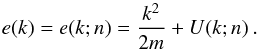 (2)We note that we assume natural units ħ= c = 1 throughout the paper. The BHF approximation for the single-particle potential U(k;n) using the continuous choice is
 ![Mathematical equation: \begin{equation} U(k;\rtheo) = \sum _{k' \,\le\, k_F} \big\langle k k'\big| G[\rtheo; e(k)+e(k')] \big|k k'\big\rangle_a \:, \label{e:ukr} \end{equation}](/articles/aa/full_html/2015/12/aa26642-15/aa26642-15-eq26.png) (3)where the matrix element is antisymmetrized, as indicated by the “a” subscript. Due to the occurrence of U(k) in Eq. (2), the coupled system of Eqs. (1) to (3) must be solved in a self-consistent manner for several Fermi momenta of the particles involved. The corresponding BHF energy per nucleon is
(3)where the matrix element is antisymmetrized, as indicated by the “a” subscript. Due to the occurrence of U(k) in Eq. (2), the coupled system of Eqs. (1) to (3) must be solved in a self-consistent manner for several Fermi momenta of the particles involved. The corresponding BHF energy per nucleon is ![Mathematical equation: \begin{equation} \frac{E}{A} = \frac{3}{5} \frac{k_F^2}{2m} + \frac{1}{2\rtheo} \sum_{k,k' \,\le\, k_F} \big\langle k k'\big|G[\rtheo; e(k)+e(k')]\big|k k'\big\rangle_a. \end{equation}](/articles/aa/full_html/2015/12/aa26642-15/aa26642-15-eq29.png) (4)In this scheme, the only input quantity we need is the bare NN interaction v in the Bethe-Goldstone Eq. (1). The nuclear EoS can be calculated with good accuracy in the Brueckner two-hole-line approximation with the continuous choice for the single-particle potential, since the results in this scheme are quite close to the calculations which include also the three-hole-line contribution (Song et al. 1998; Baldo et al. 2000b; Baldo & Burgio 2001). In the present work, we use the Argonne v18 potential (Wiringa et al. 1995) as the two-nucleon interaction. The dependence on the NN interaction, as well as a comparison with other many-body approaches, has been systematically investigated in (Baldo et al. 2012).
(4)In this scheme, the only input quantity we need is the bare NN interaction v in the Bethe-Goldstone Eq. (1). The nuclear EoS can be calculated with good accuracy in the Brueckner two-hole-line approximation with the continuous choice for the single-particle potential, since the results in this scheme are quite close to the calculations which include also the three-hole-line contribution (Song et al. 1998; Baldo et al. 2000b; Baldo & Burgio 2001). In the present work, we use the Argonne v18 potential (Wiringa et al. 1995) as the two-nucleon interaction. The dependence on the NN interaction, as well as a comparison with other many-body approaches, has been systematically investigated in (Baldo et al. 2012).
One of the well-known results of several studies, which lasted for about half a century, is that non-relativistic calculations, based on purely two-body interactions, fail to reproduce the correct saturation point of symmetric nuclear matter, and three-body forces among nucleons are needed to correct this deficiency. In our approach the TBF is reduced to a density-dependent two-body force by averaging over the position of the third particle, assuming that the probability of having two particles at a given distance is reduced according to the two-body correlation function (Baldo et al. 1997). In this work we use a phenomenological approach based on the so-called Urbana model, which consists of an attractive term due to two-pion exchange with excitation of an intermediate Δ resonance, and a repulsive phenomenological central term (Schiavilla et al. 1986). Those TBFs produce a shift of the saturation point (the minimum) of about + 1 MeV in energy. This adjustment was obtained by tuning the two parameters contained in the TBFs, and was performed to get an optimal saturation point (for details see Baldo et al. 1997). The calculated nuclear EoS conforms to several constraints required by the phenomenology of heavy ion collisions and astrophysical observational data (Taranto et al. 2013).
For computational purposes, an educated polynomial fit is performed on top of the microscopic calculation of the nuclear EoS including a fine tuning of the two parameters of the three-body forces such that the saturation point be E/A = −16 MeV at a density n0 = 0.16 fm-3. The interpolating polynomials for symmetric nuclear matter and pure neutron matter are written as 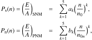 (5)where n0n = 0.155 fm-3. The values of the coefficients of the interpolating polynomials (BCP09 version of the parameters, Baldo et al. 2010) are given in Table 1.This fit is valid up to density around n = 0.4 fm-3, and it is used only for convenience. For higher density, as the ones occurring in NS cores, we use a direct numerical interpolation of the computed EoS, using the same procedure and functional form as in reference (Burgio & Schulze 2010) for a set of accurate BHF calculations. We found that the polynomial form of the EoS and the high density fit join smoothly in the interval 0.3−0.4 fm-3, for both the energy density and the pressure of the β stable matter. The overall EoS so obtained will be reported in the corresponding Tables below and used for NS calculations.The properties of infinite nuclear matter at saturation are collected in Table 2, and we see that their values agree very well with the known empirical values. The symmetry energy and the corresponding slope parameter L are two important quantities closely related to various properties of neutron stars and to the thickness of the neutron skin of nuclei (Horowitz & Piekarewicz 2001). It can be noticed that the predicted values for Esym(n0) and L lie within the recent constraints derived from the analysis of different astrophysical observations (Newton et al. 2013; Steiner et al. 2010; Lattimer & Lim 2013; Hebeler et al. 2013) and nuclear experiments (Chen et al. 2010; Tsang et al. 2012; Viñas et al. 2014).
Properties of nuclear matter at saturation predicted by the EoS of this work in comparison with the empirical ranges (Newton et al. 2013; Steiner et al. 2010; Lattimer & Lim 2013; Hebeler et al. 2013; Chen et al. 2010; Tsang et al. 2012; Viñas et al. 2014).
The BHF result can be directly employed for the calculations of the NS liquid core, where the nuclei have dissolved into their constituents, protons and neutrons. However, the description of finite nuclei and nuclear structures of a NS crust is not manageable on a fully microscopic level. Indeed, the only known tractable framework to solve the nuclear many-body problem in finite nuclei across the nuclear chart is provided by density functional theory. In order to describe finite nuclei, the BCPM energy density functional was built (Baldo et al. 2008b, 2010, 2013) based on the same microscopic BHF calculations presented before. The BCPM functional is obtained within an approximation inspired by the Kohn-Sham method (Kohn & Sham 1965). In this approach the energy is split into two parts, the first one being the uncorrelated kinetic energy, while the second one contains both the potential energy and the correlated part of the kinetic energy. An auxiliary set of A orthonormal orbitals ϕi(r,σ,q) is introduced (where A is the nucleon number and σ and q are spin and isospin indices), allowing one to write the one-body density as if it were obtained from a Slater determinant as n(r) = ∑ i,σ,q | ϕi(r,σ,q) | 2, and the uncorrelated kinetic energy as 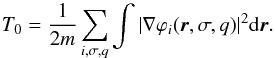 (6)To deal with the unknown form of the correlated part of the energy density functional, a strategy often followed in atomic and molecular physics is to use accurate theoretical calculations performed in a uniform system which finally are parametrized in terms of the one-body density. We use a similar approach, and we apply it to the nuclear many-body problem to obtain the BCPM functional. For this purpose we split the interacting nuclear part of the energy (EN) into bulk and surface contributions (i.e.
  ). We obtain the bulk contribution
  directly from the ab initio BHF calculations of the uniform nuclear matter system by a local density approximation. Namely, in our approach depends locally on the nucleon density n = nn + np and the asymmetry parameter β = (nn − np) / (nn + np) and reads as
 ![Mathematical equation: \begin{equation} E_{N}^{\rm bulk}[\rnum_{\rm p},\rnum_{\rm n}] = \int \big[P_s(\rtheo) (1 - \beta^2) + P_{\rm n} (\rtheo)\beta^2 \big] \rtheo {\rm d}{\vec r} , \label{bulk} \end{equation}](/articles/aa/full_html/2015/12/aa26642-15/aa26642-15-eq66.png) (7)where the polynomials Ps(n) and Pn(n) in powers of the one-body density have been introduced in Eq. (5).
(7)where the polynomials Ps(n) and Pn(n) in powers of the one-body density have been introduced in Eq. (5).
In addition to the bulk part, also surface, Coulomb, and spin-orbit contributions which are absent in nuclear matter are necessary in the interacting functional to properly describe finite nuclei. We make the simplest possible choice for the surface part of the functional by adopting the form ![Mathematical equation: \begin{eqnarray} E_{N}^{\rm surf}[\rnum_{\rm p},\rnum_{\rm n}] &=& \frac{1}{2}\sum_{q,q'}\int \int \rnum_{q}({\vec r}) v_{q,q'}({\vec r}-{\vec r'}) \rnum_{q'}({\vec r'} ){\rm d}{\vec r} {\rm d}{\vec r'} \nonumber \\ \label{surf} &&- \frac{1}{2}\sum_{q,q'} \int {\rnum_{q}({\vec r})} \rnum_{q'}({\vec r}) {\rm d}{\vec r} \int v_{q,q'}({\vec r'}) {\rm d}{\vec r'}, \end{eqnarray}](/articles/aa/full_html/2015/12/aa26642-15/aa26642-15-eq69.png) (8)where q = n,p for neutrons and protons. The second term in Eq. (8) is subtracted to not contaminate the bulk part determined from the microscopic nuclear matter calculation. For the finite range form factors we take a Gaussian shape vq,q′(r) = Vq,q′e− r2/α2, with three adjustable parameters: the range α, the strength Vp,p = Vn,n ≡ VL for like nucleons, and the strength Vn,p = Vp,n ≡ VU for unlike nucleons. The Coulomb contribution to the functional is the sum of a direct term and a Slater exchange term computed from the proton density:
(8)where q = n,p for neutrons and protons. The second term in Eq. (8) is subtracted to not contaminate the bulk part determined from the microscopic nuclear matter calculation. For the finite range form factors we take a Gaussian shape vq,q′(r) = Vq,q′e− r2/α2, with three adjustable parameters: the range α, the strength Vp,p = Vn,n ≡ VL for like nucleons, and the strength Vn,p = Vp,n ≡ VU for unlike nucleons. The Coulomb contribution to the functional is the sum of a direct term and a Slater exchange term computed from the proton density: 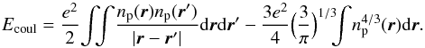 (9)As in Skyrme and Gogny forces, the spin-orbit term is a zero-range interaction vs.o. = iW0(σi + σj) × [ k′ × δ(ri − rj)k ], whose contribution to the energy reads
 ![Mathematical equation: \begin{equation} E_{\rm s.o.}= - \frac{W_0}{2}\!\int\! [ \rtheo({\vec r}) \nabla {\bf J}({\vec r})+\rnum_{\rm n}({\vec r}) \nabla {\bf J}_{\rm n}({\vec r}) + \rnum_{\rm p}({\vec r}) \nabla {\bf J}_{\rm p}({\vec r})] {\rm d}{\vec r} , \label{bcp4} \end{equation}](/articles/aa/full_html/2015/12/aa26642-15/aa26642-15-eq77.png) (10)where the uncorrelated spin density Jq for each kind of nucleon is obtained using the auxiliary set of orbitals as
(10)where the uncorrelated spin density Jq for each kind of nucleon is obtained using the auxiliary set of orbitals as ![Mathematical equation: \begin{equation} {\bf J}_q({\vec r})= -i \sum_{i,\sigma,\sigma'} \varphi_i^*({\vec r},\sigma,q) [\nabla \varphi_i({\vec r}, \sigma', q)\times \langle \sigma \,\vert\, \boldsymbol{\sigma} \,\vert\, \sigma' \rangle ]. \label{bcp5} \end{equation}](/articles/aa/full_html/2015/12/aa26642-15/aa26642-15-eq79.png) (11)Thus, the total energy of a finite nucleus is expressed as
(11)Thus, the total energy of a finite nucleus is expressed as  (12)In the calculations of open-shell nuclei we also take into account pairing correlations. The minimization procedure applied to the full functional gives a set of Hartree-like equations where the potential part includes in an effective way the overall exchange and correlation contributions. Further details of the functional can be found in (Baldo et al. 2008b, 2010, 2013).
Parameters of the Gaussian form factors and spin-orbit strength.
We note that the posited functional has only four open parameters (the strengths VL and VU, the range α of the surface term, and the spin-orbit strength W0), while the rest of the functional is derived from the microscopic BHF calculation. The four open parameters have been determined by minimizing the root-mean-square (rms) deviation σE between the theoretical and experimental binding energies of a set of well-deformed nuclei in the rare-earth, actinide, and super-heavy mass regions of the nuclear chart (Baldo et al. 2008b). The optimized values of the parameters are given in Table 3. The predictive power of the functional is then tested by computing the binding energies of 467 known spherical nuclei. A fairly reasonable rms deviation σE = 1.3 MeV between theory and experiment is found. Indeed, the rms deviations for binding energies and for charge radii of nuclei across the mass table with the BCPM functional are comparable to those obtained with highly successful nuclear mean field models such as the D1S Gogny force, the SLy4 Skyrme force, and the NL3 RMF parameter set, which for the same set of nuclei yield rms deviations σE of 1.2–1.8 MeV, see (Baldo et al. 2008b, 2010, 2013). The study of ground-state deformation properties, fission barriers, and excited octupole states with the BCPM functional (Robledo et al. 2008, 2010) shows that the deformation properties of BCPM are similar to those predicted by the D1S Gogny force, which can be considered as a benchmark to study deformed nuclei.
3. The outer crust
The outer crust of a NS is the region of the star that consists of neutron-rich nuclei and free electrons at densities approximately between 104 g/cm3, where atoms become completely ionized, and 4 × 10¹¹ g/cm3, where neutrons start to drip from the nuclei. The nuclei arrange themselves in a solid body-centred cubic (bcc) lattice in order to minimize the Coulomb repulsion and are stabilized against β decay by the surrounding electron gas. At the low densities of the beginning of the outer crust, the Coulomb lattice is populated by 56Fe nuclei. As the density of matter increases with increasing depth in the crust, it becomes energetically favourable for the system to lower the proton fraction through electron captures with the energy excess carried away by neutrinos. The system progressively evolves towards a lattice of more and more neutron-rich nuclei as it approaches the bottom of the outer crust, until the neutron drip density is reached and the inner crust of the NS begins.
3.1. Formalism for the outer crust
To describe the structure of the outer crust we follow the formalism developed by Baym, Pethick, and Sutherland (BPS; Baym et al. 1971b), as applied more recently in (Rüster et al. 2006; Roca-Maza & Piekarewicz 2008; Roca-Maza et al. 2012; see also Haensel et al. 2006; Pearson et al. 2011, and references therein). It is considered that the matter inside the star is cold and charge neutral, and that it is in its absolute ground state in complete thermodynamic equilibrium. This is a meaningful assumption for non-accreting neutron stars that have lived long enough to cool down and to reach equilibrium after their creation. In the outer crust, the energy at average baryon number density nb consists of the nuclear plus electronic and lattice contributions:  (13)where A is the number of nucleons in the nucleus, Z is the atomic number, and nb = A/V (where V stands for volume). The nuclear contribution to Eq. (13) corresponds to the mass of the nucleus, i.e. the rest mass energy of its neutrons and protons minus the nuclear binding energy:
  (14)The electronic contribution reads Eel = ℰelV, where the energy density ℰel of the electrons can be considered as that of a degenerate relativistic free Fermi gas:
 ![Mathematical equation: \begin{eqnarray} {\cal E}_{\rm el} &=& \frac{k_{\rm Fe}}{8\pi^{2}} (2k_{\rm Fe}^{2}+m_{\rm e}^{2}) \sqrt{k_{\rm Fe}^{2}+m_{\rm e}^{2}} \nonumber\\ \label{eq3} && \mbox{} - \frac{m_{\rm e}^{4}}{8\pi^{2}} \ln\Big[ \Big(k_{\rm Fe}+\sqrt{k_{\rm Fe}^{2}+m_{\rm e}^{2}}\Big) \,\Big/ m_{\rm e} \Big] , \end{eqnarray}](/articles/aa/full_html/2015/12/aa26642-15/aa26642-15-eq96.png) (15)with kFe = (3π2ne)1 / 3 being the Fermi momentum of the electrons, ne = (Z/A)nb the electron number density, and me the electron rest mass. The lattice energy can be written as
(15)with kFe = (3π2ne)1 / 3 being the Fermi momentum of the electrons, ne = (Z/A)nb the electron number density, and me the electron rest mass. The lattice energy can be written as  (16)where kFb = (3π2nb)1 / 3 = (A/Z)1 / 3kFe is the average Fermi momentum and Cl = 3.40665 × 10⁻³ for bcc lattices (Roca-Maza & Piekarewicz 2008). The lattice contribution has the form of the Coulomb energy in the nuclear mass formula with a particular prefactor and corresponds to the repulsion energy among the nuclei distributed in the bcc lattice, their attraction with the electrons, and the repulsion energy among the electrons.
The basic assumption in the calculation is that thermal, hydrostatic, and chemical equilibrium is reached in each layer of the crust. As no pressure is exerted by the nuclei, only the electronic and lattice terms contribute to the pressure in the outer crust (Baym et al. 1971b). Therefore, we have  (17)where
  is the Fermi energy of the electrons including their rest mass. One has to find the nucleus that at a certain pressure minimizes the Gibbs free energy per particle, or chemical potential, μ = G/A = (E − TS) /A + P/nb (Baym et al. 1971b). As far as the system can be assumed at zero temperature in good approximation, since the electronic Fermi energy is much larger that the temperature of the star, the quantity to be minimized is given by
  (18)For a fixed pressure, Eq. (18) is minimized with respect to the mass number A and the atomic charge Z of the nucleus in order to find the optimal configuration. The nuclear masses M(A,Z) needed in Eq. (18) can be taken from experiment if they are available or calculated using nuclear models.
3.2. Equation of state of the outer crust
Although thousands of nuclear masses are experimentally determined not far from stability, the masses of very neutron-rich nuclei are not known. We used in Eq. (18) the measured masses whenever available. For the unknown masses, we performed deformed Hartree-Fock-Bogoliubov calculations with the BCPM energy density functional, which has been constructed from the microscopic BHF calculations as described in Sect. 2. We took the experimental data of masses from the most recent atomic mass evaluation, i.e. the AME2012 evaluation (Audi et al. 2012). As the field of high-precision mass measurements of unstable neutron-rich nuclei continues to advance in the radioactive beam facilities worldwide (Thoennessen 2013), better constraints can be placed on the composition of the outer crust. Thus, we also included in our calculation the mass of 82Zn recently determined by a Penning-trap measurement at ISOLDE-CERN (Wolf et al. 2013). Being the most neutron-rich N = 50 isotone known to date, 82Zn is an important nucleus in the study of the NS outer crust (Wolf et al. 2013).
The calculated composition of the outer crust (neutron and proton numbers of the equilibrium nuclei) vs. the average baryon density nb is displayed in Fig. 1. After the 56Fe nucleus that populates the outer crust up to nb = 5 × 10⁻⁹ fm-3 (8 × 10⁶ g/cm3), the composition profile exhibits a sequence of plateaus. The effect is related with the enhanced nuclear binding for magic nucleon numbers, i.e. Z = 28 in the Ni plateau that occurs at intermediate densities in Fig. 1, and N = 50 and N = 82 in the neutron plateaus that occur at higher densities. Along a neutron plateau, such as N = 50, the nuclei experience electron captures that reduce the proton number, resulting in a staircase structure of shells of increasingly neutron-rich isotones, until the jump to the next neutron plateau (N = 82) takes place. The composition of the crust is determined by the experimental masses up to densities around 2.5 × 10⁻⁵ fm-3 (4 × 10¹⁰ g/cm3). At higher densities, model masses need to be used because the relevant nuclei are more neutron rich and their masses are not measured.
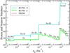 |
Fig. 1 Neutron (N) and proton (Z) numbers of the predicted nuclei in the outer crust of a neutron star using the experimental nuclear masses (Audi et al. 2012; Wolf et al. 2013) when available and the BCPM energy density functional or the FRDM mass formula (Möller et al. 1995) for the unmeasured masses. |
The results for the composition in the high-density part of the outer crust from the microscopic BCPM model can be seen in Fig. 1. They are shown along with the results from the macroscopic-microscopic finite-range droplet model (FRDM) of Möller, Nix et al. (Möller et al. 1995) that was fitted with high accuracy to the thousands of experimental masses available at the time it was published. Despite BCPM has no more than four fitted parameters (for reference, the sophisticated macroscopic-microscopic models such as the FRDM (Möller et al. 1995) and the Duflo-Zuker model (Duflo & Zuker 1995) have tens of adjustable parameters), the predictions of BCPM are overall quite in consonance with those of the FRDM. In particular, the jump to the N = 82 plateau is predicted at practically the same density. Some differences are found, though, in the width of the shell of 78Ni before the N = 82 plateau, and in the fact that BCPM reaches the neutron drip with a (very thin) shell of 114Se, while the FRDM reaches the neutron drip with a shell of 118Kr. We note that at the base of the outer crust (neutron drip) the baryon density, mass density, pressure, and electron chemical potential of the equilibrium configuration in BCPM are nb = 2.62 × 10⁻⁴ fm-3, ϵ = 4.37 × 10¹¹ g/cm3, P = 4.84 × 10⁻⁴ MeV/fm3, and μe = 26.09 MeV, respectively. These values are close (cf. Table I of Roca-Maza & Piekarewicz 2008) to the results computed using the highly successful FRDM (Möller et al. 1995) and Duflo-Zuker (Duflo & Zuker 1995) models, what gives us confidence that the BCPM energy density functional is well suited for extrapolating to the neutron-rich regions.
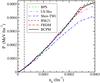 |
Fig. 2 Pressure in the outer crust against baryon density using the experimental nuclear masses (Audi et al. 2012; Wolf et al. 2013) when available and the BCPM energy density functional or the FRDM mass formula (Möller et al. 1995) for the unmeasured masses. Also shown is the pressure from models BSk21, BPS, Lattimer-Swesty (LS-Ska), and Shen et al. (Shen-TM1) (see text for details). The dashed vertical line indicates the approximate end of the experimentally constrained region. |
Composition and equation of state of the outer crust.
In Fig. 2 we display the EoS, or pressure-density relationship, of the outer crust obtained from the experimental masses plus BCPM, and from the experimental masses plus the FRDM. One observes small jumps in the density for particular values of the pressure. They are associated with the change from an equilibrium nucleus to another in the composition. During this change the pressure and the chemical potential remain constant, implying a finite variation of the baryon density (Baym et al. 1971b; Rüster et al. 2006; Haensel et al. 2006; Pearson et al. 2011). After the region constrained by the experimental masses (marked by the dashed vertical line in Fig. 2), the pressures of BCPM (black solid line) and the FRDM (red dashed line) extrapolate very similarly, with only some differences appreciated by the end of the outer crust. Our results for the composition and EoS of the outer crust are given in Table 4. The quantities ϵ and Γ in this table are, respectively, the mass density of matter and the adiabatic index Γ = (nb/P) (dP/ dnb).
Also plotted in Fig. 2 is the pressure in the outer crust from some popular EoSs that model the complete structure of the NS. The figure is drawn up to nb = 3 × 10⁻⁴ fm-3, thus comprising the change from the outer crust to the inner crust in order to allow comparison of the EoSs also in this region (notice, however, that inner crust results are not available for the FRDM). We show in Fig. 2 the EoS from the recent BSk21 Skyrme nuclear effective force (Pearson et al. 2012; Fantina et al. 2013; Potekhin et al. 2013; Goriely et al. 2010) tabulated in (Potekhin et al. 2013). The parameters of this force were fitted (Goriely et al. 2010) to reproduce with high accuracy almost all known nuclear masses, and to various physical conditions including the neutron matter EoS from microscopic calculations. We see in Fig. 2 that after the experimentally constrained region, the BSk21 pressure is similar to the BCPM and FRDM results, with just some displacement around the densities where the composition changes from a nucleus to the next one. In the seminal work of BPS (Baym et al. 1971b) the nuclear masses for the outer crust were provided by an early semi-empirical mass table. The corresponding EoS is seen to display a similar pattern with the BCPM, FRDM, and BSk21 results in Fig. 2. The EoS by Lattimer & Swesty (1991), taken here in its Ska version (Lattimer 2015; LS-Ska), and the EoS by (Shen et al. 1998b,a; Sumiyoshi 2015; Shen-TM1) were computed with, respectively, the Skyrme force Ska and the relativistic mean-field model TM1. In the two cases the calculations of masses are of semiclassical type and A and Z vary in a continuous way. Therefore, these EoSs do not present jumps at the densities associated with a change of nucleus in the crust. Beyond this feature, the influence of shell effects in the EoS is rather moderate because to the extent that the pressure at the densities of interest is largely determined by the electrons, small changes of the atomic number Z compared with its semiclassical estimate modify only marginally the electron density and, consequently, the pressure. The LS-Ska EoS shows good agreement with the previously discussed models, with some departure from them in the transition to the inner crust. The largest discrepancies in Fig. 2 are observed with the Shen-TM1 EoS that in this region predicts a softer crustal pressure with density than the other models.
4. The inner crust: formalism
Below the outer crust, the inner crust starts at a density about 4 × 10¹¹ g/cm3, where nuclei have become so neutron rich that neutrons drip in the environment, and extends until the NS core. The structure of the inner crust consists of a Coulomb lattice of nuclear clusters permeated by the gases of free neutrons and free electrons. This is a unique system that is not accessible to experiment because of the presence of the free neutron gas. The fraction of free neutrons increases with growing density of matter. At the bottom layers of the inner crust the equilibrium nuclear shape may change from sphere, to cylinder, slab, tube (cylindrical hole), and bubble (spherical hole) before going into uniform matter. These shapes are generically known as “nuclear pasta”.
Full quantal Hartree-Fock (HF) calculations of the nuclear structures in the inner crust are complicated by the treatment of the neutron gas and the eventual need to deal with different geometries. As a result, large scale calculations of the inner crust and nuclear pasta have been performed very often with semiclassical methods such as the CLDM (Lattimer & Swesty 1991; Douchin & Haensel 2001) or the Thomas-Fermi (TF) approximation and their variants, employing effective forces for the nuclear interaction, see (Haensel et al. 2006; Chamel & Haensel 2008) for reviews. Calculations of TF type, including pasta phases, have been carried out both in the non-relativistic (Oyamatsu 1993; Gögelein & Müther 2007; Onsi et al. 2008; Pearson et al. 2012) and in the relativistic (Cheng et al. 1997; Shen et al. 1998b,a; Avancini et al. 2008; Grill et al. 2012) nuclear mean-field theories.
In this work we apply the self-consistent TF approximation to describe the inner crust for two reasons. First, our main aim is to obtain the EoS of the neutron star, which is largely driven by the neutron gas and where the contribution of shell corrections is to some extent marginal. Second, the semiclassical methods, as far as they do not contain shell effects, are well suited to describe non-spherical shapes, i.e. pasta phases, as we shall discuss below. Nevertheless, it is to be mentioned that in the case of spherical symmetry, shell corrections for protons in the inner crust may be introduced perturbatively on top of the semiclassical results via the Strutinsky shell-correction method. These corrections have been included in the calculations of the inner crust by the Brussels-Montreal group (Chamel et al. 2011; Pearson et al. 2012; Fantina et al. 2013; Potekhin et al. 2013) with the BSk19–BSk21 Skyrme forces (Goriely et al. 2010). Shell effects can be taken into account self-consistently using the HF method. Indeed, HF calculations of inner crust matter were performed in spherical WS cells in the pioneering work of Negele & Vautherin (1973). Pairing effects in the inner crust can have important consequences to describe, e.g. pulsar glitches phenomena or the cooling of NS. Pairing correlations have been included in BCS and HFB calculations of the inner crust in the spherical WS approach, see for instance (Pizzochero et al. 2002; Sandulescu et al. 2004; Baldo et al. 2007; Grill et al. 2011; Pastore et al. 2011) and references therein, and also in the BCS theory of anisotropic multiband superconductivity beyond the WS approach (Chamel et al. 2010). These works are mainly devoted to investigate the superfluid properties of NS inner crusts and only, to our knowledge, in (Baldo et al. 2007) the EoS of the inner crust including pairing correlations was reported.
It must be mentioned as well that the formation and the properties of nuclear pasta have been investigated in three-dimensional HF (Gögelein & Müther 2007; Pais & Stone 2012; Schuetrumpf et al. 2014) and TF (Okamoto et al. 2013) calculations in cubic boxes that avoid any assumptions on the geometry of the system. Generally speaking, the results of these calculations observe the usual pasta shapes but additional complex morphologies can appear as stable or metastable states at the transitions between shapes (Gögelein & Müther 2007; Pais & Stone 2012; Schuetrumpf et al. 2014; Okamoto et al. 2013). Techniques based on Monte Carlo and molecular dynamics simulations, which do not impose a periodicity or symmetry of the system unlike the WS approximation, have also been applied to study nuclear pasta, see (Horowitz et al. 2004, 2015; Watanabe et al. 2009; Schneider et al. 2013) and references therein. (We note that some of the quoted three-dimensional simulation calculations are for pasta in supernova matter rather than in cold neutron-star matter.) These calculations are highly time consuming and a detailed pressure-vs.-density relation for the whole inner crust is not yet available.
4.1. Self-consistent Thomas-Fermi description of the inner crust of a neutron star
In this section we describe the method used for computing the structure and the EoS of the inner crust with the BCPM energy density functional. Although a summary of the approach has been presented elsewhere (Baldo et al. 2014), here we provide a more complete report of the formalism.
The total energy of an ensemble of A − Z neutrons, Z protons, and Z electrons in a spherical Wigner-Seitz (WS) cell of volume  can be expressed as
 ![Mathematical equation: \begin{eqnarray} E &=& {E(A,Z, R_{\rm c})} \,=\, \int_{V_{\rm c}}\!\! \Big[{\cal H}\left(\rnum_{\rm n},\rnum_{\rm p}\right) + m_{\rm n}\rnum_{\rm n} + m_{\rm p}\rnum_{\rm p} \nonumber \\[2mm] \label{eq1} && \mbox{} + {\cal E}_{\rm el}\left(\rnum_{\rm e}\right) + {\cal E}_{\rm coul}\left(\rnum_{\rm p},\rnum_{\rm e}\right) + {\cal E}_{\rm ex}\left(\rnum_{\rm p},\rnum_{\rm e}\right) \Big] {\rm d}{\vec r} . \end{eqnarray}](/articles/aa/full_html/2015/12/aa26642-15/aa26642-15-eq132.png) (19)The term
(19)The term  is the contribution of the nuclear energy density, without the nucleon rest masses. In our approach it reads
 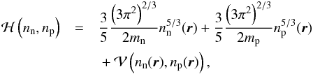 (20)where the neutron and proton kinetic energy densities are written in the TF approximation and
  is the interacting part provided by the BCPM nuclear energy density functional (see Sect. 2), which contains bulk and surface contributions. The term
  in Eq. (19) is the relativistic energy density due to the motion of the electrons, including their rest mass. Since at the densities prevailing in neutron star inner crust the Fermi energy of the electrons is much higher than the Coulomb energy, we computed ℰel using the energy density of a uniform relativistic Fermi gas given by Eq. (15). The term
  in Eq. (19) is the Coulomb energy density from the direct part of the proton-proton, electron-electron, and proton-electron interactions. Assuming that the electrons are uniformly distributed, this term can be written as
 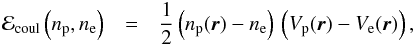 (21)with
 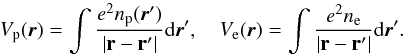 (22)We did calculations where we allowed the profile of the electron density to depend locally on position. However, we found this to have a marginal influence on our results for compositions and energies and decided to proceed with a uniform distribution for the electrons. Lastly, the term ℰex(np,ne) in Eq. (19) is the exchange part of the proton-proton and electron-electron interactions treated in Slater approximation:
 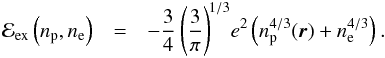 (23)We consider the matter within a WS cell of radius Rc and perform a fully variational calculation of the total energy E(A,Z,Rc) of Eq. (19) imposing charge neutrality and an average baryon density nb = A/Vc. The fact that the nucleon densities are fully variational differs from some other TF calculations carried out with non-relativistic nuclear models (Oyamatsu 1993; Gögelein & Müther 2007; Onsi et al. 2008; Pearson et al. 2012) that use parametrized trial neutron and proton densities in the minimization. TF calculations of the inner crust with fully variational densities using relativistic nuclear mean-field models have been reported in the literature (Cheng et al. 1997; Shen et al. 1998b,a; Avancini et al. 2008; Grill et al. 2012).
Taking functional derivatives of Eq. (19) with respect to the particle densities and including the conditions of charge neutrality and constant average baryon density with suitable Lagrange multipliers, leads to the variational equations 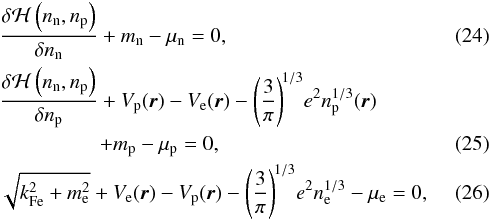 plus the β-equilibrium condition
  (27)which is imposed along with the constraints of charge neutrality and fixed average baryon density in the cell. We note that in this work the chemical potentials μn, μp, and μe include the rest mass of the particle.
Equations (24)–(27) are solved self-consistently in a WS cell of specified size Rc following the method described in (Sil et al. 2002) and the energy is calculated from Eq. (19). Next, a search of the optimal size of the cell for the considered average baryon density nb is performed by repeating the calculation for different values of Rc, in order to find the absolute minimum of the energy per baryon for that nb. This can be a delicate numerical task because the minimum of the energy is usually rather flat as a function of the cell radius Rc (or, equivalently, as a function of the baryon number A) and the energy differences may be between a few keV and a few eV.
In order to obtain the EoS of the inner crust we have to compute the pressure. The derivation of the expression of the pressure in this region of the NS is given in Appendix A. As shown in the appendix (also see Pearson et al. 2012), in the inner crust the pressure assumes the form 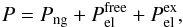 (28)where Png is the pressure of the gas of dripped neutrons,
  is the pressure of free electron gas, and
  is a corrective term from the electron Coulomb exchange. That is, the pressure in the inner crust is exerted by the neutron and electron gases in which the nuclear structures are embedded. On the other hand, in Appendix B we show explicitly that when the minimization of the energy per unit volume with respect to the radius of the WS cell is attained, subjected to an average density nb and charge neutrality, the Gibbs free energy G = PV + E per particle equals the neutron chemical potential, i.e. G/A = μn. This result provides an alternative way to extract the pressure from the knowledge of the neutron chemical potential and the energy.
The same formalism described for spherical nuclei can be applied to obtain solutions for spherical bubbles (hollow spheres). Assuming the appropriate geometry, the method can be used in a similar way for other shapes (nuclear pasta), as discussed in the next subsection.
4.2. Pasta phases: cylindrical and planar geometries
The method of solving Eqs. (24)–(27) can be extended to deal with WS cells having cylindrical symmetry (rods or “nuclear spaghetti”) or planar symmetry (slabs or “nuclear lasagne”). The length of the rods and the area of the slabs in the inner crust of a neutron star are effectively infinite. The calculations for these non-spherical geometries are simplified if one also considers the unit cells as rods and slabs of infinite extent in the direction perpendicular to the base area of the rods and to the width of the slabs, respectively. That is, the corresponding WS cells are taken as rods of finite radius Rc and length L → ∞, and as slabs of finite width 2Rc and transverse area S → ∞. With this choice of geometries, the number of particles and energy per unit length (rods) or area (slabs) are finite. By taking dV = 2πLrdr for rods and dV = Sdx for slabs in Eq. (19), the energy calculations are reduced to one-variable integrals over the finite size Rc of the WS cell (i.e. from 0 to Rc in a circle of radius Rc in the case of rods, and from −Rc to + Rc along the x direction for slabs). The calculation of the Coulomb potentials is likewise simplified. In the case of rods the direct Coulomb potential can be written as ![Mathematical equation: \begin{equation} V_{\rm p}\left(r\right) = -4{\pi}e^{2}\! \left[\ln r \!\int_{0}^{r}\!\! r'\rnum_{\rm p}(r'){\rm d}r' + \int_{r}^{ R_{\rm c}}\!\! r' \ln r' \rnum_{\rm p}(r'){\rm d}r'\right] \label{eq11} \end{equation}](/articles/aa/full_html/2015/12/aa26642-15/aa26642-15-eq165.png) (29)for protons, and as
(29)for protons, and as  (30)for the uniform electron distribution. In the case of slabs these potentials read
 ![Mathematical equation: \begin{equation} V_{\rm p}\left(x\right)= -4{\pi}e^{2}\! \left[x \!\int_{0}^{x}\!\! \rnum_{\rm p}(x'){\rm d}x' + \int_{x}^{ R_{\rm c}}\!\! x'\rnum_{\rm p}(x'){\rm d}x'\right], \label{eq9} \end{equation}](/articles/aa/full_html/2015/12/aa26642-15/aa26642-15-eq167.png) (31)and
(31)and  (32)The other piece of the energy that depends on the geometry of the WS cell is the nuclear surface contribution, which is given by Eq. (8) for the BCPM energy density functional. In the case of spherical nuclei, performing the angular integration, the surface energy density of Eq. (8) can be recast as
 ![Mathematical equation: \begin{eqnarray} \label{eq14} {\cal E}_\textrm{surf}\left(\rnum_{q},\rnum_{q'}\right) & = & \frac{\pi}{2}\sum_{q,q'} \alpha^{2} {V}_{q,q'}\rnum_{q}(r) \nonumber \\ &&\quad \times \bigg[\frac{1}{r} \int_{0}^{\infty} \! \rnum_{q'}(r') \Big(e^{{-(r - r')^{2}}/{\alpha^{2}}} -e^{{-(r + r')^{2}}/{\alpha^{2}}}\Big) ~r'~ {\rm d}r' \nonumber \\ &&\quad - \pi^{1/2}\alpha\rnum_{q'}(r)\bigg] . \end{eqnarray}](/articles/aa/full_html/2015/12/aa26642-15/aa26642-15-eq169.png) (33)For rods the nuclear surface contribution to the energy density is given by
(33)For rods the nuclear surface contribution to the energy density is given by ![Mathematical equation: \begin{eqnarray} \label{eq15} {\cal E}_\textrm{surf}\left(\rnum_{q},\rnum_{q'}\right) & = & \frac{\pi}{2}\sum_{q,q'} \alpha^2 {V}_{q,q'}\rnum_q(r) \nonumber \\ &&\quad \times \bigg[ \frac{2}{\alpha} \pi^{1/2} e^{-r^{2}/\alpha^{2}} \!\! \int_{0}^{\infty} \! \rnum_{q'}(r')e^{-r'^{2}/\alpha^{2}}I_{0} \Big(\frac{2rr'}{\alpha^{2}}\Big) ~r'~ {\rm d}r' \nonumber \\ &&\quad - \pi^{1/2}\alpha \rnum_{q'}(r)\bigg] , \end{eqnarray}](/articles/aa/full_html/2015/12/aa26642-15/aa26642-15-eq170.png) (34)where I0 is the modified Bessel function, while for slabs it is given by
(34)where I0 is the modified Bessel function, while for slabs it is given by ![Mathematical equation: \begin{eqnarray} \label{eq16} {\cal E}_\textrm{surf}\left(\rnum_{q},\rnum_{q'}\right) &= & \frac{\pi}{2}\sum_{q,q'}\alpha^{2}{V}_{q,q'}\rnum_q(x) \nonumber \\ &&\quad \times \bigg[\int_{-\infty}^{\infty} \rnum_{q'}(x')e^{-\left(x-x'\right)^{2}/\alpha^{2}} {\rm d}x' \nonumber \\ &&\quad- \pi^{1/2}\alpha \rnum_{q'}(x)\bigg] . \end{eqnarray}](/articles/aa/full_html/2015/12/aa26642-15/aa26642-15-eq172.png) (35)As happens with spherical nuclei and spherical bubbles, the equations corresponding to cylindrical rods can be similarly applied to obtain the solutions for tube shapes (hollow rods).
(35)As happens with spherical nuclei and spherical bubbles, the equations corresponding to cylindrical rods can be similarly applied to obtain the solutions for tube shapes (hollow rods).
5. The inner crust: results
5.1. Analysis of the self-consistent solutions
To compute the EoS of a neutron-star inner crust we need to determine the optimal configuration of the WS cell, i.e. the shape and composition that yield the minimal energy per baryon, as a function of the average baryon density nb. This is done for each nb value following the method explained in the previous section. In Fig. 3 we display the results for the minimal energy per baryon E/A in the different shapes. The energy per baryon is shown relative to the value in uniform neutron-proton-electron (npe) matter in order to be able to appreciate the energy separations between shapes. Our set of considered shapes consists of spherical droplets, cylindrical rods, slabs, cylindrical tubes, and spherical bubbles.
As can be seen in Fig. 3, it was possible to obtain solutions for rods and slabs starting at densities as low as nb ~ 0.005 fm-3. Solutions at lower crustal densities, i.e. from the transition density between the outer crust and the inner crust until nb = 0.005 fm-3, were obtained for spherical droplets only. These solutions are not plotted in Fig. 3 for visual purposes of the rest of the figure. We note that at a density nb = 0.0003 fm-3 immediately after the neutron drip point, i.e. at the beginning of the inner crust, the difference E/A − (E/A)npe is of −2.5 MeV. For tube and bubble shapes, solutions could be obtained for crustal densities higher than about 0.07 fm-3, where the system is not far from uniform matter.
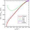 |
Fig. 3 Energy per baryon of different shapes relative to uniform npe matter as a function of baryon density in the inner crust. |
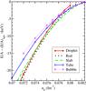 |
Fig. 4 Energy per baryon of different shapes relative to uniform npe matter as a function of baryon density in the high-density region of the inner crust. |
The spherical droplet configuration is the energetically most favourable shape all the way up to nb ~ 0.065 fm-3, see Fig. 3. When the crustal density reaches ~0.065 fm-3 (approximately 1014 g/cm3), the nucleus occupies a significant fraction of the cell volume and it may happen that non-spherical structures have lower energy than the spherical droplets (Ravenhall et al. 1983; Lorenz et al. 1993; Oyamatsu 1993; Haensel et al. 2006; Chamel & Haensel 2008). We show in Fig. 4 the high-density region between nb = 0.07 fm-3 and nb = 0.0825 fm-3, where the TF-BCPM model predicts the appearance of non-spherical shapes as optimal configurations. Indeed, the first change of nuclear shape occurs at nb = 0.067 fm-3 from droplets to rods. It can be seen in Fig. 4 that the cylindrical shape is the energetically favoured configuration up to a crustal density of 0.076 fm-3 where a second change takes place to the planar slab shape. As the density of the crustal matter increases further, the energy per baryon of tubes and bubbles becomes progressively closer to that of the slabs. Very close to the crust-core transition, estimated to occur in the TF-BCPM model at nb = 0.0825 fm-3, there are successive shape changes from slabs to tubes at nb = 0.082 fm-3 and to spherical bubbles at almost 0.0825 fm-3. At this latter density, the energy per baryon of the self-consistent TF bubble solution and that of uniform matter differ by barely −200 eV (in comparison, the value of E/A − mn is of 8.3 MeV). In summary, as compiled in Table 5, the TF-BCPM model predicts that the sequence of shapes in the inner crust changes from spherical droplets to rods, slabs, tubes, and spherical bubbles. This is in consonance with the ordering of pasta phases reported in previous TF calculations (Oyamatsu 1993; Avancini et al. 2008; Grill et al. 2012). It can be noticed that the consideration of pasta shapes renders the transition to the core somewhat smoother. The energy differences between the most bound shape and the spherical solution at the same density are, though, small and do not exceed 1−1.5 keV per nucleon.
Baryon density of the successive changes of energetically favourable topology in the inner crust.
A typical landscape of solutions is illustrated in Fig. 5 where, for a density nb = 0.077 fm-3, the energy per baryon relative to the neutron rest mass is shown as a function of the size of the WS cell for the various shapes. Usually, the curves for a given shape are flat around their minimum. For example, in the case of spherical droplets in Fig. 5, a 1% deviation of Rc from the value of the minimum implies a shift of merely 25 eV in E/A, but it changes the baryon number by as much as 25 units. Sufficiently close points have to be computed in order to determine precisely the Rc value (equivalently, the A value) that corresponds to the minimal energy per baryon. On the other hand, at high crustal densities the differences among the energy per baryon of the minima of the various shapes (quoted in brackets in Fig. 5) are small; e.g. the minima of the slab and rod solutions in Fig. 5 differ by 190 eV.
Figure 6 displays the cell size Rc and the proton fraction xp = Z/A of the equilibrium configurations against nb for the different shapes in our calculation. Rc shows a nearly monotonic downward trend when the density increases, in agreement with other studies of NS inner crusts (Oyamatsu 1993; Onsi et al. 2008; Pearson et al. 2012; Avancini et al. 2008; Grill et al. 2012). The size of the cell has a significant dependence on the geometry of the nuclear structures, as seen by comparing Rc of the different shapes. In the spherical solutions, the cell radius decreases from almost 45 fm at nb = 0.0003 fm-3 to 13.7 fm at nb = 0.08 fm-3 near the transition to the core. As regards the proton fraction xp, it takes quite similar values for the various cell geometries in the ranges of densities where we obtained solutions for the respective shapes. Beyond a density of the order of 0.02 fm-3 the proton fraction shows a weak change with density, and after nb ~ 0.05 fm-3 it smoothly tends to the value in uniform npe matter. For the spherical droplet solutions, we find that xp rapidly decreases from 31% at nb = 0.0003 fm-3 to ~3% at nb = 0.02 fm-3. It afterward remains almost constant, presenting a minimum value of 2.75% at nb = 0.045 fm-3 and then a certain increase up to 3.2% at the last densities before the core.
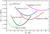 |
Fig. 5 The minimum energy per baryon relative to the neutron mass for different shapes as a function of the cell size Rc at an average baryon density nb = 0.077 fm-3. The value of the absolute minimum for each shape is shown in MeV in brackets. |
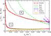 |
Fig. 6 Radius Rc of the Wigner-Seitz cell and proton fraction xp = Z/A (given in percentage) in different geometries with respect to the baryon density. |
Taking into account that except for densities close to the crust-core transition the spherical shape is the energetically preferred configuration, and when it is not, the energy differences are fairly small, we restrict the discussion about the A and Z values in the WS cells to spherical nuclei. Figure 7 depicts the evolution with nb of A and Z of the equilibrium spherical solutions. The numerical values are collected in Table 6. When free neutrons begin to appear in the crust the number of nucleons contained in a cell quickly increases from A = 113 up to a maximum A ≃ 1100 at nb = 0.025 fm-3. From this density onwards, A shows a slowly decreasing trend (with a relative plateau around nb ~ 0.05 fm-3) till A ≃ 820 at nb ≃ 0.07 fm-3, and finally it presents an increase approaching the core. We see in Fig. 7 that the results for the atomic number Z in the inner crust show an overall smooth decrease as a function of nb and a final slight increase before the transition to the core in agreement with the behaviour of A. The range of Z values lies between an upper value Z ≃ 36 at nb ≃ 0.01 fm-3 and a lower value Z ≃ 25 at nb ≃ 0.07 fm-3. We note that in our calculation the mass and atomic numbers vary continuously and are not restricted to integer values because we have used the TF approximation which averages shell effects. The same fact explains that the atomic number Z of the optimal configurations does not correspond to proton magic numbers, as it happens when proton shell corrections are included in the calculations (Negele & Vautherin 1973; Baldo et al. 2007; Chamel et al. 2011; Pearson et al. 2012; Fantina et al. 2013; Potekhin et al. 2013). However, as we have seen from the flatness of E/A with respect to A (or Rc) around the minima in the discussion of Fig. 5, the resulting EoS is robust against the details of the composition.
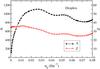 |
Fig. 7 Mass number A (left vertical scale) and atomic number Z (right vertical scale) corresponding to spherical nuclei with respect to the baryon density. |
Composition of the inner crust.
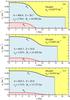 |
Fig. 8 a) Optimal density profile of neutrons nn and protons np for spherical nuclear droplets at average baryon density nb = 0.0475 fm-3. The associated baryon and proton numbers, proton fraction xp = Z/A in percentage, and radius of the cell are shown. The vertical dashed line marks the location of the end of the WS cell. b) The same for nb = 0.065 fm-3. c) The same for nb = 0.076 fm-3. |
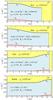 |
Fig. 9 a) Optimal density profile of neutrons nn and protons np for rod shapes at average baryon density nb = 0.076 fm-3. The associated baryon and proton numbers, proton fraction xp = Z/A in percentage, and radius of the cell are shown. The vertical dashed line marks the location of the end of the WS cell. b) The same for slab shapes. c) The same for tube shapes. d) The same for bubble shapes. We note that the scale on the horizontal axis is the same in Figs. 9c and a, and in Figs. 9d and 8c. |
Before leaving this section, in Fig. 8 we display the spatial dependence of the self-consistent neutron and proton density profiles for the optimal solutions in spherical WS cells with average baryon densities nb = 0.0475 fm-3, 0.065 fm-3, and 0.076 fm-3. It is observed that in denser matter the size of the WS cell decreases, as we discussed previously, and that the amount of free neutrons in the gas increases, as expected. It can be seen that the nuclear surface is progressively washed out with increasing average baryon density as the nucleon distributions become more uniform. At high nb the density profile inside the WS cell extends towards the edge of the cell, pointing out that the WS approximation may be close to its limits of validity (Negele & Vautherin 1973; Chamel et al. 2007; Baldo et al. 2007; Pastore et al. 2011; Gögelein & Müther 2007; Newton & Stone 2009). Although the proton number Z is similar for the three average baryon densities of Fig. 8, the local distribution of the protons is very different in the three cases. In Fig. 8c the proton density profile extends more than 3 fm farther from the origin than in Fig. 8a, while the central value of the proton density has decreased by more than a factor 2, hinting at the fact that the neutrons have a strong drag effect on the protons. Figure 9 presents the nucleon density profiles obtained for cylindrical and planar geometries at the same average density nb = 0.076 fm-3 as in Fig. 8c. From Figs. 8c (droplets), 9a (rods), and 9b (slabs) we see that the size of the WS cells decreases with decreasing dimensionality, i.e. Rc,droplet>Rc,rod>Rc,slab. At high average densities near the crust-core transition, nucleons inside the WS cell can arrange themselves in such a way that the region of higher density is concentrated at the edge of the cell, leaving the uniform region of lower density in the inner part of the cell. This distribution of nucleons corresponds to the cylindrical tube and spherical bubble configurations. In Figs. 9c and d, we plot the neutron and proton density profiles of the optimal solution for tubes and bubbles at nb = 0.076 fm-3. At equal average density, the size of the cells containing tubes and bubbles is larger than the size of the cells accommodating rods and droplets, respectively, as can be appreciated by comparing Fig. 9a for rods with Fig. 9c for tubes, and Fig. 8c for droplets with Fig. 9d for bubbles. As a consequence of this fact and of the effectively larger value of the integration factors 2πr and 4πr2 when the densities are accumulated near the edge of the cell, the total number of nucleons and the atomic number in the tube and bubble cells is about 1.5−2 times larger than in their rod and droplet counterparts. The proton fraction xp = Z/A is, however, practically the same for all geometries.
5.2. Equation of state of the inner crust
The energy per baryon in the inner crust predicted by the BCPM functional is displayed against the average baryon density in Fig. 10. The result is compared with other calculations available in the literature. This comparison will be, at the same time, useful to discriminate popular EoSs used in neutron-star modeling among each other. We show in Fig. 10 the results of the quantal calculations of Negele & Vautherin (1973; label NV) and of Baldo et al. (2007; label Moskow). These two EoSs of the inner crust include shell effects and in the case of Moskow also pairing correlations. In addition to these models, we compare with some of the EoSs that have been devised to describe the complete neutron-star structure. The EoS by Baym et al. (1971a,b; label BBP), the EoS by Lattimer & Swesty (1991) in its Ska version (Lattimer 2015; label LS-Ska), and the EoS by Douchin & Haensel (2001; label DH-SLy4) were all obtained using the CLDM model to describe the inner crust. The results by Shen et al. (1998a,b; Sumiyoshi 2015; label Shen-TM1) were computed in the TF approach with trial nucleon density distributions. Finally, in the recent EoS of the Brussels-Montreal BSk21 force (Pearson et al. 2012; Fantina et al. 2013; Potekhin et al. 2013; Goriely et al. 2010) the inner crust was calculated in the extended TF approach with trial nucleon density profiles and with proton shell corrections incorporated by means of the Strutinsky method.
The energy in the inner crust is largely influenced by the properties of the neutron gas and, therefore, the EoS of neutron matter of the different calculations plays an essential role. The NV calculation (Negele & Vautherin 1973) is based on a local energy density functional that closely reproduces the Siemens-Pandharipande EoS of neutron matter (Siemens & Pandharipande 1971) in the low-density regime. The Moskow calculation (Baldo et al. 2007) employs a semi-microscopic energy density functional obtained by combining the phenomenological functional of Fayans et al. (2000) inside the nuclear cluster with a microscopic part calculated in the Brueckner theory with the Argonne v18 potential (Wiringa et al. 1995) to describe the neutron environment in the low-density regime (Baldo et al. 2004). The BBP calculation (Baym et al. 1971a,b) gives the EoS based on the Brueckner calculations for pure neutron matter of Siemens (Siemens & Pandharipande 1971). The LS-Ska (Lattimer & Swesty 1991; Lattimer 2015) and DH-SLy4 (Douchin & Haensel 2001) EoSs were constructed using the Skyrme effective nuclear forces Ska and SLy4, respectively. The SLy4 Skyrme force (Chabanat et al. 1998) was parametrized, among other constraints, to be consistent with the microscopic variational calculation of neutron matter of Wiringa et al. (1988) above the nuclear saturation density. The Shen-TM1 EoS (Shen et al. 1998b,a; Sumiyoshi 2015) was computed using the relativistic mean field parameter set TM1 for the nuclear interaction. The calculations of LS (Lattimer & Swesty 1991; Lattimer 2015) and Shen et al. (Shen et al. 1998b,a; Sumiyoshi 2015) are the two EoS tables in more widespread use for astrophysical simulations. The BSk21 EoS (Pearson et al. 2012; Fantina et al. 2013; Potekhin et al. 2013; Goriely et al. 2010) is based on a Skyrme force with the parameters accurately fitted to the known nuclear masses and constrained, among various physical conditions, to the neutron matter EoS derived within modern many-body approaches which include the contribution of three-body forces.
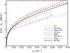 |
Fig. 10 Energy per baryon relative to the neutron rest mass as a function of the average baryon density in the inner crust for the BCPM functional and other EoSs. |
It can be realized in Fig. 10 that the energies per baryon predicted in the inner crust by the BCPM functional and by the NV calculation (Negele & Vautherin 1973) lie close over a wide range of densities, as also noticed before (Schuck & Viñas 2013). The result of the BBP model (Baym et al. 1971a,b) agrees similarly with BCPM and NV at low densities, while above nb ~ 0.02 fm-3 it predicts somewhat larger energies than BCPM and NV. The DH-SLy4 calculation (Douchin & Haensel 2001) consistently predicts throughout the inner crust the largest energies of all the models analyzed in Fig. 10. The energies of the BSk21 calculation (Pearson et al. 2012; Fantina et al. 2013; Potekhin et al. 2013; Goriely et al. 2010) are very close to those of DH-SLy4 up to nb ~ 0.03−0.04 fm-3. When the transition to the core is approached, the BSk21 energies become closer to the BCPM and NV results than to the DH-SLy4 result. The Moskow calculation (Baldo et al. 2007) predicts lower energies than the previous models. However, the most remarkable differences are found with the results of the LS-Ska (Lattimer & Swesty 1991; Lattimer 2015) and Shen-TM1 (Shen et al. 1998b,a; Sumiyoshi 2015) calculations. It seems evident that the BCPM functional, as well as the results of the models constrained by some information of microscopic calculations (NV, Moskow, BBP, DH-SLy4, and BSk21), predicts overall substantially larger energies per baryon in the inner crust than the LS-Ska and Shen-TM1 models that do not contain explicit information of microscopic neutron matter calculations.
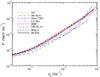 |
Fig. 11 Pressure as a function of the average baryon density in the inner crust for the BCPM functional and other EoSs. The figure starts at nb = 3 × 10⁻⁴ fm-3 where Fig. 2 ended. |
The pressure in the crust is an essential ingredient entering the Tolman-Oppenheimer-Volkoff equations (Shapiro & Teukolsky 1983) that determine the mass-radius relation in neutron stars. The crustal pressure has also significant implications for astrophysical phenomena such as pulsar glitches (Piekarewicz et al. 2014). As expressed in Eq. (28), the pressure in the inner crust is provided by the free gases of the electrons and of the interacting dripped neutrons (aside from a correction from Coulomb exchange). We note, however, that the pressure obtained in a WS cell in the inner crust differs from the value in homogeneous npe matter in β-equilibrium at the same average density nb owing to the lattice effects, which influence the electron and neutron gases. The lattice effects take into account the presence of nuclear structures in the crust and are automatically included in the self-consistent TF calculation.
The pressure predictions in the inner crust by the BCPM functional are shown in Fig. 11 in comparison with the predictions by the same models discussed in Fig. 10. The initial baryon density in Fig. 11 corresponds to the last density shown in Fig. 2 when we studied the EoS of the outer crust in Sect. 3. In the inner crust, the pressure from the BCPM functional is comparable in general to the results of the NV, BBP, DH-SLy4, and BSk21 calculations. Particular agreement is observed in the inner crust regime between the BCPM and BSk21 pressures up to relatively high crustal densities. In contrast, large differences are found when the BCPM pressure is compared with the values from the Moskow, LS-Ska, and Shen-TM1 models. As the crust-core transition is approached, these differences can be as large as a factor of two, which may have an influence on the predictions of the mass-radius relationship of neutron stars, particularly in small mass stars. In addition to the spherical shape, we have evaluated the pressure for the non-spherical WS cells and the hollow shapes in the regime of high average baryon densities using the BCPM functional. However, on the one hand, as noted before, the pasta phases appear as the preferred configuration only in a relatively narrow range of densities between nb ≃ 0.067 fm-3 and nb ≃ 0.08 fm-3. On the other hand, the differences between the pressure of the spherical shape and the pressure from the successively favoured shapes are small, generally of the order of 1–2 keV/fm3 or less. Therefore, as we did in (Baldo et al. 2014), we have taken as a representative result for the whole inner crust the pressure calculated in the spherical droplet configurations. The corresponding EoS data are collected in Table 7.
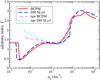 |
Fig. 12 Adiabatic index from the EoSs of BCPM and DH-SLy4 (Douchin & Haensel 2001). The result calculated in homogeneous npe matter is also shown. |
Equation of state of the inner crust.
An important quantity, which actually determines the response of the crust to the compression or decompression of matter, is the so-called adiabatic index 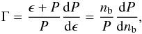 (36)where P is the pressure, ϵ the mass density of matter, and nb the average baryon density. In Fig. 12 we plot the adiabatic index from the BCPM and DH-SLy4 (Douchin & Haensel 2001) EoS in the region from the last layers of the outer crust until a density well within the NS core (discussed in the next section). In the bottom layers of the outer crust the pressure is governed almost entirely by the ultra-relativistic electron gas, so that the value of Γ is quite close to 4 / 3. At the neutron drip point, Γ sharply decreases by more than a factor of two due to the dripped neutrons that strongly soften the EoS. The just dripped neutrons contribute to the average baryon density but exert very little pressure. In the inner crust region, when the density increases the adiabatic index grows because the pressure of the neutron gas also increases. In our EoS the adiabatic index of the inner crust changes from Γ ≃ 0.45 after the neutron drip point up to Γ ≃ 2.1 near the crust-core transition (nb ≃ 0.08 fm-3).
In the same Fig. 12 we report Γ computed in a single phase of homogeneous npe matter in β-equilibrium. It is observed that Γ in the inner crust almost coincides with the result in a single phase for densities between nb ~ 0.01 fm-3 and 0.05 fm-3. Above 0.05 fm-3, the adiabatic index of homogeneous npe matter grows faster than in the inner crust, because the latter is softened by the presence of nuclear structures and the coexistence between the two phases. The predictions of the DH-SLy4 EoS (Douchin & Haensel 2001) for Γ in the inner crust show a similar qualitative behaviour but differ quantitatively from the BCPM EoS. For example, at the bottom of the inner crust the adiabatic index in the DH-SLy4 EoS is Γ ~ 1.6, while it takes a value of 2.1 in BCPM. This difference seems to indicate that the interacting part of the neutron gas at densities near the crust-core transition is weaker in SLy4 than in the BCPM functional (also see in this respect Fig. 1 of Baldo et al. 2004). When the transition to the core is reached, Γ increases in a discontinuous way from 2.1 to 2.5 in the BCPM EoS, due to the change from two phases to a single phase. With higher density in the core, the adiabatic index stiffens from the increase of the repulsive contributions in the nucleon-nucleon interaction. It is interesting to note that Γ exhibits a small sharp drop at the muon onset, which in BCPM is located at a density nb ≃ 0.13 fm-3. It arises from the appearance of muons that replace some high-energy electrons and effectively reduce the pressure at this density. At higher densities Γ remains roughly constant, which is partly due to the increasing proton fraction in the npeμ matter of the core.
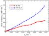 |
Fig. 13 Shear modulus from the EoS of BCPM and DH-SLy4 (Douchin & Haensel 2001). |
Quasi-periodic oscillations in giant flares emitted by highly-magnetized neutron stars are signatures of the fundamental seismic shear mode, which is specially sensitive to the nuclear physics of neutron-star crusts (Steiner & Watts 2009; Sotani et al. 2012). An important quantity for describing shear modes is the effective shear modulus μ. It can be estimated from the known formula for a bcc Coulomb crystal at zero temperature (Steiner & Watts 2009; Sotani et al. 2012; Strohmayer et al. 1991):  (37)where Z and Rc are the proton number and the radius of a spherical WS cell having average baryon density nb. In Fig. 13 we display the effective shear modulus from our calculation with the BCPM functional along with the result from DH-SLy4 (Douchin & Haensel 2001). Because the elasticity for pasta phases, with the exception of spherical bubbles, is expected to be much lower than for spherical nuclei (Sotani et al. 2012), we restrict the plot in Fig. 13 to spherical configurations, i.e. up to an average density nb = 0.067 fm-3 where pasta phases start to be the most favourable configuration in the BCPM calculation. The effective shear modulus (37) depends on the composition of the crust through the proton number Z, which has a rather smooth variation along the inner crust with BCPM (see Fig. 7), and on the size of the WS cells that decreases from the neutron drip till the bottom layers of the inner crust (see Fig. 6). The difference between the predictions of BCPM and SLy4 for μ in Fig. 13 increases with density. At the higher densities of Fig. 13 the DH-SLy4 result is about twice the BCPM result, pointing out the different composition and sizes of the WS cells in the DH-SLy4 (Douchin & Haensel 2001) and BCPM models. Lower values of μ for the BCPM case point in the direction of lower frequencies of the fundamental shear mode, but a complete analysis is beyond the scope of the present paper.
6. The liquid core
The EoS for the liquid core is derived in the framework of the Brueckner-Bethe-Goldstone theory (Baldo 1999) as described in Sect. 2. The Argonne v18 potential (Wiringa et al. 1995) is used as the NN interaction and three-body forces based on the so-called Urbana model are included in the calculation to reproduce the nuclear matter saturation point (Schiavilla et al. 1986; Baldo et al. 1997, 2012; Taranto et al. 2013).
In order to study the structure of the NS core, we have to calculate the composition and the EoS of cold, neutrino-free, catalyzed matter. As we discussed in the Introduction, we consider a NS with a core of nucleonic matter without hyperons or other exotic particles. We require that it contains charge neutral matter consisting of neutrons, protons, and leptons (e−, μ−) in beta equilibrium, and compute the EoS for charge neutral and beta-stable matter in the following standard way (Baldo et al. 1997; Shapiro & Teukolsky 1983). The Brueckner calculation yields the energy density of lepton/baryon matter as a function of the different partial densities,  (38)where we have used ultrarelativistic and relativistic approximations for the energy densities of electrons and muons (Shapiro & Teukolsky 1983), respectively. In practice, it is sufficient to compute only the binding energy of symmetric nuclear matter and pure neutron matter, since within the BHF approach it has been verified (Baldo et al. 1998, 2000a; Lejeune et al. 1986; Zuo et al. 1999; Bombaci & Lombardo 1991) that a parabolic approximation for the binding energy of nuclear matter with arbitrary proton fraction xp = np/nb, nb = nn + np, is well fulfilled,
  (39)where the symmetry energy Esym can be expressed in terms of the difference of the energy per particle between pure neutron (xp = 0) and symmetric (xp = 0.5) matter:
  (40)Knowing the energy density Eq. (38), the various chemical potentials (of the species i = n,p,e,μ) can be computed straightforwardly,
  (41)and the equations for beta-equilibrium,
 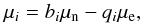 (42)(bi and qi denoting baryon number and charge of species i) and charge neutrality,
  (43)allow one to determine the equilibrium composition ni at given baryon density nb and finally the EoS,
 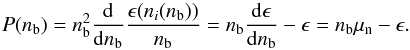 (44)
(44)
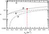 |
Fig. 14 Populations vs. nucleon density for the BCPM EoS discussed in the text. The full red dot indicates the value of the nucleon density at which direct Urca processes set in. |
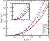 |
Fig. 15 Pressure vs. nucleon density for the several EoSs discussed in the text, i.e. the BCPM (solid, red), the BSk21 (dot-dashed-dashed, magenta), the Lattimer-Swesty (Ska, dashed, blue), the Shen (dot-dashed, green), and the Douchin-Haensel (SLy4, dot-dot-dashed, black). A detail of the region between nb = 0.05 fm-3 and 0.30 fm-3 is shown in the inset. The incompressibility coefficients at nuclear saturation density for these models are K = 214 MeV (BCPM), 230 MeV (SLy4), 246 MeV (BSk21), 263 MeV (Ska), and 281 MeV (Shen). |
Populations of the liquid core.
In Table 8 the populations are reported for a fixed nucleon density, and are plotted in Fig. 14. The full red dot indicates the value of the nucleon density at which direct Urca processes set in. We remind that Urca processes play an important role in the neutron star cooling (Lattimer et al. 1991; Yakovlev et al. 2001). We notice that the BCPM EoS predicts a density onset value close to 0.53 fm-3, and therefore with our EoS medium mass NS can cool very quickly. In Table 9 we report the corresponding EoS, which is represented in Fig. 15 by a red solid curve. We notice a remarkable similarity with the EoS derived by (Douchin & Haensel 2001; black curve), based on the effective nuclear interaction SLy4 of Skyrme type. On the other hand, a strong difference with the Lattimer-Swesty EoS (dashed blue), the Shen EoS (dot-dashed, green), and the BSk21 EoS (dot-dashed-dashed, magenta) is observed at high densities. We recall that the pressures from the Lattimer-Swesty EoS and the Shen EoS had already been found to differ significantly from BCPM and SLy4 for the matter at subsaturation density in the inner crust (see discussion of Fig. 11). However, the BCPM and SLy4 pressures in the inner crust showed a concordance with BSk21 that remains within the core region up to about 0.2 fm-3 (see inset of Fig. 15) but is not maintained in the extrapolation to higher densities, where the BSk21 and Lattimer-Swesty models predict the stiffest EoSs of Fig. 15.
Equation of state of the liquid core.
Once the EoS of the nuclear matter is known, one can solve the Tolman-Oppenheimer-Volkoff (Shapiro & Teukolsky 1983) equations for spherically symmetric NS: 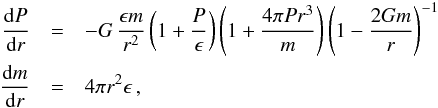 (45)where G is the gravitational constant, P the pressure, ϵ the energy density, m the mass enclosed within a radius r, and r the (relativistic) radius coordinate. To close the equations we need the relation between pressure and energy density, P = P(ϵ), i.e. the EoS. The integration of these equations produces the mass and radius of the star for given central density. It turns out that the mass of the NS has a maximum value as a function of radius (or central density), above which the star is unstable against collapse to a black hole. The value of the maximum mass depends on the nuclear EoS, so that the observation of a mass higher than the maximum mass allowed by a given EoS simply rules out that EoS. We display in Fig.16 the relation between mass and radius (left panel) and central density (right panel). The observed trend is consistent with the equations of state displayed in Fig. 15. As expected, when the stiffness increases the NS central density decreases for a given mass. The considered EoSs are compatible with the largest mass observed up to now, i.e. MG = 2.01 ± 0.04 M⊙ in PSR J0348+0432 (Antoniadis et al. 2013), and displayed in Fig. 16, along with the previously observed mass of PSR J1614-2230 (Demorest et al. 2010) having MG = 1.97 ± 0.04 M⊙. We also notice that the maximum mass calculated with the BCPM and the SLy4 EoSs is characterized by a radius of about 10 km, which is somewhat smaller than the radius calculated with the other considered EoSs. Recent analyses of observations on quiescent low-mass X-ray binaries (QLMXB) (Guillot & Rutledge 2014) and X-ray bursters (Güver & Özel 2013) seem to point in this direction, though more studies could be needed (Lattimer & Steiner 2014b). For a NS of 1.5 solar masses, the BCPM EoS predicts a radius of 11.63 km (see Table 10), in line with the recent analysis shown in Ozel et al. (2015); see also Chen & Piekarewicz (2015). For completeness, we also display in the orange hatched band the probability distribution for MG and R deduced from five PRE (Photospheric Radius Expansion) burst sources and five QLMXB sources, after a Bayesian analysis (Lattimer & Steiner 2014a). We see that, except the Shen EoS, all EoSs are compatible with the observational data. High-precision determinations of NS radii that may be achieved in the future by planned observatories such as the Neutron star Interior Composition ExploreR (NICER) (Arzoumanian et al. 2014), should prove a powerful complement to maximum masses for resolving the equation of state of the dense matter of compact stars.
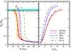 |
Fig. 16 Gravitational mass, in units of the solar mass M⊙ = 2×1033 g vs. radius (left panel) and central density (right panel) in units of the saturation density n0 = 0.16 fm-3. See text for details. |
Properties of the maximum mass configuration for a given EoS.
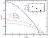 |
Fig. 17 Density profiles for fixed mass configurations, i.e. MG = Mmax (solid blue curve), MG = 1.4 M⊙ (dashed red curve), and MG = 1.0 M⊙ (dot-dashed green curve). Full dots indicate the onset of the crust. In the inset the crust thickness is displayed for each fixed gravitational mass. See text for details. |
In Fig. 17 we report the density profiles for three values of the mass calculated with the EoS of the present work. The transition density between the inner crust and the core is indicated by a dot along the curves. Accordingly, in the inset we report the ratio of the crust thickness and the total radius of the star. These informations can be relevant for phenomena occurring in the star, like glitches and deep crustal heating.
7. Summary and outlook
We have derived a unified equation of state for neutron stars with a microscopic model which is able to describe on the same physical framework, both the core and the crust regions. We describe the neutron star structure based on modern Brueckner-Hartree-Fock calculations performed in symmetric and neutron matter. These microscopic calculations are also the basis of the Barcelona-Catania-Paris-Madrid energy density functional, devised to reproduce accurately the nuclear binding energies throughout the nuclear mass table. This functional is used to describe the finite nuclei present in the crust of neutron stars. To our knowledge, this is the first time that a whole equation of state directly connected to microscopic results has been reported in the literature.
The equation of state in the outer crust is obtained using the Baym-Pethick-Sutherland model, which requires the knowledge of atomic masses near the neutron drip line. In our calculation we use the experimental masses, when they are available, together with the values provided by a deformed Hartree-Fock-Bogoliubov calculation performed with the Barcelona-Catania-Paris-Madrid energy density functional to estimate the unknown masses. We find that for average densities above ϵ ≃ 5 × 10¹⁰ g cm-3, where the experimental masses are unknown, the composition of the outer crust is similar to the one predicted by the Finite Range Droplet Model of Möller and Nix.
We describe the structure of the inner crust in the Wigner-Seitz approximation using the selfconsistent Thomas-Fermi method together with the Barcelona-Catania-Paris-Madrid energy density functional. Electrons are considered as a relativistic Fermi gas with a constant density, which fill up the whole Wigner-Seitz cell. To obtain the optimal configuration in a cell for a given average density and size, the energy per baryon is minimized by solving self-consistently the coupled Euler-Lagrange equations for the neutron, proton and electron densities. To obtain the most stable configuration for a given average density, an additional minimization with respect to the size of the Wigner-Seitz cell is required.
Because the Thomas-Fermi model does not include shell corrections, the mass and atomic numbers corresponding to the configuration of minimal energy vary smoothly as a function of the average density. For spherical shapes, the mass number along the whole inner crust lies in the range between A ≃ 110 and A ≃ 850 with a maximum around A = 1100 for an average density nb ≃ 0.025 fm-3. The atomic number shows a roughly decreasing tendency from Z ≃ 35 at the neutron drip up to Z ≃ 25 at the crust-core transition.
Using the same Thomas-Fermi model, we have also investigated the possible existence of pasta phases. To this end we have computed the minimal energy per baryon in Wigner-Seitz cells with planar and cylindrical geometries for average densities above nb ≃ 0.005 fm-3 and for tube and bubble configurations from nb = 0.07 fm-3 and nb = 0.072 fm-3, respectively, until the crust-core transition density, which is reached in our model at nb = 0.0825 fm-3. Our model predicts that up to average densities of nb = 0.067 fm-3, spherical nuclei are the minimal energy configurations. With growing average densities, our model predicts the successive appearance of rods, slabs, tubes and spherical bubbles as the most stable shape.
To describe the core of neutron stars within our model we consider uniform matter containing neutrons, protons, electrons and eventually muons in β-equilibrium, which determines the asymmetry of the homogeneous system. To derive the Equation of State in the core, we use directly the microscopic Brueckner-Hartree-Fock results in symmetric and neutron matter, which allow us to easily obtain the pressure as a function of the density in this regime. The npeμ model is expected to be valid at least up to densities of about three times the saturation density, above which exotic matter could appear. However, we restricted ourselves to a NS nucleonic core and extrapolated the npeμ matter to higher densities as was done in earlier literature (Wiringa et al. 1988; Douchin & Haensel 2001).
We have compared the predictions of our Equation of State, derived on a microscopic basis from the outer crust to the core, with the results obtained using some well-known Equations of State available in the literature. Our Equation of State clearly differs from the results provided by the Lattimer and Swesty and Shen models, obtained in a more phenomenological way and widely used in astrophysical calculations. Our calculation agrees reasonably well in the crust with the predictions of the Equation of State of Douchin and Haensel and with the results of the BSk21 model of the Brussels-Montreal group, both based on Skyrme forces but including some microscopic information, and also shows a remarkable similarity with the former in the core but differs more of the latter in this region of the neutron stars.
The mass and radius of non-rotating neutron stars are obtained by solving the Tolman-Oppenheimer-Volkov equations. Our model predicts a maximal mass of about two solar masses, compatible with the largest mass measured up to now, and a radius of about 10 km. The radius obtained with our model is within the range of values estimated from observations of quiescent low-mass X-ray binaries and from type I X-ray bursts. The mass-radius relationship computed with our model is comparable to the results obtained using the Equation of State of Douchin and Haensel above the standard mass of neutron stars (1.4 solar masses) and differs from the predictions of the BSk21, Lattimer and Swesty and Shen models in this domain of neutron star masses. The maximal masses of the neutron stars are determined by the stiffness of the equation of State at high densities. As can be observed in Figs. 15 and 16, where the equation of State, the maximal mass and the central density obtained using the different models considered in this work are displayed, when the stiffness increases the maximum value of the mass increases and, for a fixed mass, the central density decreases.
However, there are some theoretical caveats to be considered. It can be expected that quark matter appears in the centre of massive NS. To describe these “hybrid” NS one needs to know the quark matter EoS. Many models for the deconfined quark matter produce a too soft EoS to support a NS of mass compatible with observations (Burgio et al. 2002a,b; Baldo et al. 2003, 2008a; Maieron et al. 2004; Nicotra et al. 2006; Chen et al. 2011). The quark-quark interaction in the deconfined phase must be more repulsive in order to stiffen the EoS, and indeed, with a suitable quark-quark interaction, mixed quark-nucleon matter can have an EoS compatible with two solar masses or more (Alford et al. 2013). An additional problem arises if strange matter is introduced in the NS matter. It turns out that BHF calculations using realistic hyperon-nucleon interactions known in the literature produce a too soft NS matter EoS and the maximum mass is reduced to values well below the observational limit (Schulze et al. 2006; Schulze & Rijken 2011). Although relativistic mean field models can be adjusted to accomodate NS masses larger than two solar masses (Oertel et al. 2015), and additional terms in the hyperon-nucleon interaction can provide a possible solution (Yamamoto et al. 2014), this “hyperon puzzle” has to be considered still open (Fortin et al. 2015). In any case the nuclear EoS with the inclusion of quarks and/or hyperons at high density must reach a stiffness at least similar to the EoS with only nucleons if the two solar masses problem has to be overcome.
The full BCPM EoS from the outer crust to the core in a tabulated form as a function of the baryon density as well as some other useful information is given in the text as well as supplementary material. There are different improvements that would be welcome but are left for a future work. In particular, we shall take into account shell effects and pairing correlations for protons in order to obtain a more accurate information about the compositions of the different WS cells along the inner crust. This can be done in a perturbative way on top of the TF results by using different techniques such as the Strutinsky integral method developed by Pearson and coworkers. On the other hand, the self-consistent TF-BCPM model is well suited for performing calculations at finite temperature, which can be of interest to investigate the melting point of the crystal structure. Another natural extension of this work using the TF formalism at finite temperature can be to obtain the EoS in the conditions of supernova matter.
Acknowledgments
We are indebted to Prof. L. M. Robledo for providing the deformed HFB results needed in the outer crust calculations. M.C., B.K.S., and X.V. have been partially supported by Grants Nos. FIS2011-24154 and FIS2014-54672-P from the Spanish MINECO and FEDER, Grant No. 2014SGR-401 from Generalitat de Catalunya, the Spanish Consolider-Ingenio 2010 Programme CPAN CSD2007-00042, and the project MDM-2014-0369 of ICCUB (Unidad de Excelencia María de Maeztu) from MINECO. B.K.S. greatly acknowledges the financial support from Grant No. CPAN10-PD13 from CPAN (Spain). M.B. and G.F.B. warmly thank Dr. P. Shternin for pointing us out some inaccuracies in the manuscript. The authors also wish to acknowledge the “NewCompStar” COST Action MP1304.
References
- Alford, M. G., Han, S., & Prakash, M. 2013, Phys. Rev. D, 88, 083013 [NASA ADS] [CrossRef] [Google Scholar]
- Antoniadis, J., Freire, P., Wex, N., et al. 2013, Science, 340, 1233232 [Google Scholar]
- Arzoumanian, Z., Gendreau, K. C., Baker, C. L., et al. 2014, in SPIE Conf. Ser., 9144, 20 [Google Scholar]
- Audi, G., Wang, M., Wapstra, A., et al. 2012, Chinese Phys. C, 36, 1287 [Google Scholar]
- Avancini, S. S., Menezes, D. P., Alloy, M. D., et al. 2008, Phys. Rev. C, 78, 015802 [NASA ADS] [CrossRef] [Google Scholar]
- Baldo, M. 1999, Nuclear Methods and The Nuclear Equation of State (Singapore: World Scientific) [Google Scholar]
- Baldo, M., & Burgio, G. F. 2001, in Physics of Neutron Star Interiors, eds. D. Blaschke, N. K. Glendenning, & A. Sedrakian (Berlin: Springer Verlag), Lect. Notes Phys., 578, 1 [Google Scholar]
- Baldo, M., & Fukukawa, K. 2014, Phys. Rev. Lett., 113, 242501 [NASA ADS] [CrossRef] [PubMed] [Google Scholar]
- Baldo, M., Bombaci, I., & Burgio, G. F. 1997, A&A, 328, 274 [NASA ADS] [Google Scholar]
- Baldo, M., Burgio, G. F., & Schulze, H.-J. 1998, Phys. Rev. C, 58, 3688 [NASA ADS] [CrossRef] [Google Scholar]
- Baldo, M., Burgio, G. F., & Schulze, H.-J. 2000a, Phys. Rev. C, 61, 055801 [NASA ADS] [CrossRef] [Google Scholar]
- Baldo, M., Giansiracusa, G., Lombardo, U., & Song, H. Q. 2000b, Phys. Lett. B, 473, 1 [NASA ADS] [CrossRef] [Google Scholar]
- Baldo, M., Buballa, M., Burgio, G. F., et al. 2003, Phys. Lett. B, 562, 153 [NASA ADS] [CrossRef] [Google Scholar]
- Baldo, M., Maieron, C., Schuck, P., & Viñas, X. 2004, Nucl. Phys. A, 736, 241 [NASA ADS] [CrossRef] [Google Scholar]
- Baldo, M., Saperstein, E. E., & Tolokonnikov, S. V. 2007, Eur. Phys. J. A, 32, 97 [NASA ADS] [CrossRef] [EDP Sciences] [Google Scholar]
- Baldo, M., Burgio, G. F., Castorina, P., Plumari, S., & Zappalà, D. 2008a, Phys. Rev. D, 78, 063009 [NASA ADS] [CrossRef] [Google Scholar]
- Baldo, M., Schuck, P., & Viñas, X. 2008b, Phys. Lett. B, 663, 390 [NASA ADS] [CrossRef] [Google Scholar]
- Baldo, M., Robledo, L., Schuck, P., & Viñas, X. 2010, J. Phys. G Nucl. Phy., 37, 064015 [NASA ADS] [CrossRef] [Google Scholar]
- Baldo, M., Polls, A., Rios, A., Schulze, H.-J., & Vidaña, I. 2012, Phys. Rev. C, 86, 064001 [NASA ADS] [CrossRef] [Google Scholar]
- Baldo, M., Robledo, L. M., Schuck, P., & Viñas, X. 2013, Phys. Rev. C, 87, 064305 [NASA ADS] [CrossRef] [Google Scholar]
- Baldo, M., Burgio, G. F., Centelles, M., Sharma, B. K., & Viñas, X. 2014, Phys. At. Nucl., 77, 1157 [Google Scholar]
- Baym, G., Bethe, H. A., & Pethick, C. J. 1971a, Nucl. Phys. A, 175, 225 [NASA ADS] [CrossRef] [Google Scholar]
- Baym, G., Pethick, C., & Sutherland, P. 1971b, ApJ, 170, 299 [Google Scholar]
- Bombaci, I., & Lombardo, U. 1991, Phys. Rev. C, 44, 1892 [NASA ADS] [CrossRef] [Google Scholar]
- Burgio, G. F., & Schulze, H.-J. 2010, A&A, 518, A17 [NASA ADS] [CrossRef] [EDP Sciences] [Google Scholar]
- Burgio, G. F., Baldo, M., Sahu, P. K., Santra, A. B., & Schulze, H.-J. 2002a, Phys. Lett. B, 526, 19 [NASA ADS] [CrossRef] [Google Scholar]
- Burgio, G. F., Baldo, M., Sahu, P. K., & Schulze, H.-J. 2002b, Phys. Rev. C, 66, 025802 [NASA ADS] [CrossRef] [Google Scholar]
- Carbone, A., Polls, A., & Rios, A. 2013, Phys. Rev. C, 88, 044302 [NASA ADS] [CrossRef] [Google Scholar]
- Chabanat, E., Bonche, P., Haensel, P., Meyer, J., & Schaeffer, R. 1998, Nucl. Phys. A, 635, 231 [NASA ADS] [CrossRef] [Google Scholar]
- Chamel, N., & Haensel, P. 2008, Liv. Rev. Relat., 11, 10 [Google Scholar]
- Chamel, N., Naimi, S., Khan, E., & Margueron, J. 2007, Phys. Rev. C, 75, 055806 [NASA ADS] [CrossRef] [Google Scholar]
- Chamel, N., Goriely, S., Pearson, J. M., & Onsi, M. 2010, Phys. Rev. C, 81, 045804 [NASA ADS] [CrossRef] [Google Scholar]
- Chamel, N., Fantina, A. F., Pearson, J. M., & Goriely, S. 2011, Phys. Rev. C, 84, 062802 [Google Scholar]
- Chen, W.-C., & Piekarewicz, J. 2015, Phys. Rev. Lett., 115, 161101 [NASA ADS] [CrossRef] [PubMed] [Google Scholar]
- Chen, L.-W., Ko, C. M., Li, B.-A., & Xu, J. 2010, Phys. Rev. C, 82, 024321 [NASA ADS] [CrossRef] [Google Scholar]
- Chen, H., Baldo, M., Burgio, G. F., & Schulze, H.-J. 2011, Phys. Rev. D, 84, 105023 [NASA ADS] [CrossRef] [Google Scholar]
- Cheng, K. S., Yao, C. C., & Dai, Z. G. 1997, Phys. Rev. C, 55, 2092 [NASA ADS] [CrossRef] [Google Scholar]
- Coraggio, L., Holt, J. W., Itaco, N., et al. 2014, Phys. Rev. C, 89, 044321 [NASA ADS] [CrossRef] [Google Scholar]
- Demorest, P. B., Pennucci, T., Ransom, S. M., Roberts, M. S. E., & Hessels, J. W. T. 2010, Nature, 467, 1081 [NASA ADS] [CrossRef] [PubMed] [Google Scholar]
- Douchin, F., & Haensel, P. 2001, A&A, 380, 151 [NASA ADS] [CrossRef] [EDP Sciences] [Google Scholar]
- Drischler, C., Somà, V., & Schwenk, A. 2014, Phys. Rev. C, 89, 025806 [NASA ADS] [CrossRef] [Google Scholar]
- Duflo, J., & Zuker, A. P. 1995, Phys. Rev. C, 52, 23 [Google Scholar]
- Ekström, A., Baardsen, G., Forssén, C., et al. 2013, Phys. Rev. Lett., 110, 192502 [NASA ADS] [CrossRef] [PubMed] [Google Scholar]
- Ekström, A., Jansen, G. R., Wendt, K. A., et al. 2015, Phys. Rev. C, 91, 051301 [NASA ADS] [CrossRef] [Google Scholar]
- Entem, D. R., & Machleidt, R. 2003, Phys. Rev. C, 68, 041001 [NASA ADS] [CrossRef] [Google Scholar]
- Epelbaum, E., Hammer, H.-W., & Meißner, U.-G. 2009, Rev. Mod. Phys., 81, 1773 [NASA ADS] [CrossRef] [Google Scholar]
- Fantina, A. F., Chamel, N., Pearson, J. M., & Goriely, S. 2013, A&A, 559, A128 [NASA ADS] [CrossRef] [EDP Sciences] [Google Scholar]
- Fayans, S. A., Tolokonnikov, S. V., Trykov, E. L., & Zawischa, D. 2000, Nucl. Phys. A, 676, 49 [NASA ADS] [CrossRef] [Google Scholar]
- Fortin, M., Zdunik, J. L., Haensel, P., & Bejger, M. 2015, A&A, 576, A68 [NASA ADS] [CrossRef] [EDP Sciences] [Google Scholar]
- Gögelein, P., & Müther, H. 2007, Phys. Rev. C, 76, 024312 [NASA ADS] [CrossRef] [Google Scholar]
- Goriely, S., Chamel, N., & Pearson, J. M. 2010, Phys. Rev. C, 82, 035804 [NASA ADS] [CrossRef] [Google Scholar]
- Grangé, P., Lejeune, A., Martzolff, M., & Mathiot, J.-F. 1989, Phys. Rev. C, 40, 1040 [NASA ADS] [CrossRef] [Google Scholar]
- Grill, F., Margueron, J., & Sandulescu, N. 2011, Phys. Rev. C, 84, 065801 [NASA ADS] [CrossRef] [Google Scholar]
- Grill, F., Providência, C., & Avancini, S. S. 2012, Phys. Rev. C, 85, 055808 [NASA ADS] [CrossRef] [Google Scholar]
- Guillot, S., & Rutledge, R. E. 2014, ApJ, 796, L3 [Google Scholar]
- Güver, T., & Özel, F. 2013, ApJ, 765, L1 [Google Scholar]
- Haensel, P., Potekhin, A. Y., & Yakovlev, D. G. 2006, Neutron Stars 1: Equation of State and Structure (New York: Springer) [Google Scholar]
- Hebeler, K., & Schwenk, A. 2010, Phys. Rev. C, 82, 014314 [NASA ADS] [CrossRef] [Google Scholar]
- Hebeler, K., Bogner, S. K., Furnstahl, R. J., Nogga, A., & Schwenk, A. 2011, Phys. Rev. C, 83, 031301 [NASA ADS] [CrossRef] [Google Scholar]
- Hebeler, K., Lattimer, J. M., Pethick, C. J., & Schwenk, A. 2013, ApJ, 773, 11 [NASA ADS] [CrossRef] [Google Scholar]
- Hempel, M., & Schaffner-Bielich, J. 2010, Nucl. Phys. A, 837, 210 [NASA ADS] [CrossRef] [Google Scholar]
- Holt, J. D., Menéndez, J., & Schwenk, A. 2013, Phys. Rev. Lett., 110, 022502 [NASA ADS] [CrossRef] [PubMed] [Google Scholar]
- Horowitz, C. J., & Piekarewicz, J. 2001, Phys. Rev. Lett., 86, 5647 [NASA ADS] [CrossRef] [PubMed] [Google Scholar]
- Horowitz, C. J., Pérez-García, M. A., & Piekarewicz, J. 2004, Phys. Rev. C, 69, 045804 [NASA ADS] [CrossRef] [Google Scholar]
- Horowitz, C. J., Berry, D. K., Briggs, C. M., et al. 2015, Phys. Rev. Lett., 114, 031102 [NASA ADS] [CrossRef] [PubMed] [Google Scholar]
- Kohn, W., & Sham, L. J. 1965, Phys. Rev., 140, 1133 [NASA ADS] [CrossRef] [MathSciNet] [Google Scholar]
- Laehde, T., Epelbaum, E., Krebs, H., et al. 2013, PoS(LATTICE 2013)231 [Google Scholar]
- Lattimer, J. M. 2015, EoS tables available at http://www.astro.sunysb.edu/lattimer/EOS/main.html [Google Scholar]
- Lattimer, J. M., & Lim, Y. 2013, ApJ, 771, 51 [Google Scholar]
- Lattimer, J. M., & Steiner, A. W. 2014a, Eur. Phys. J. A, 50, 40 [NASA ADS] [CrossRef] [EDP Sciences] [Google Scholar]
- Lattimer, J. M., & Steiner, A. W. 2014b, ApJ, 784, 123 [NASA ADS] [CrossRef] [Google Scholar]
- Lattimer, J. M., & Swesty, D. F. 1991, Nucl. Phys. A, 535, 331 [NASA ADS] [CrossRef] [Google Scholar]
- Lattimer, J. M., Prakash, M., Pethick, C. J., & Haensel, P. 1991, Phys. Rev. Lett., 66, 2701 [NASA ADS] [CrossRef] [PubMed] [Google Scholar]
- Lejeune, A., Grange, P., Martzolff, M., & Cugnon, J. 1986, Nucl. Phys. A, 453, 189 [NASA ADS] [CrossRef] [Google Scholar]
- Leutwyler, H. 1994, Ann. Phys., 235, 165 [Google Scholar]
- Li, Z. H., & Schulze, H.-J. 2008, Phys. Rev. C, 78, 028801 [NASA ADS] [CrossRef] [Google Scholar]
- Li, Z. H., Lombardo, U., Schulze, H.-J., & Zuo, W. 2008, Phys. Rev. C, 77, 034316 [NASA ADS] [CrossRef] [Google Scholar]
- Lorenz, C. P., Ravenhall, D. G., & Pethick, C. J. 1993, Phys. Rev. Lett., 70, 379 [NASA ADS] [CrossRef] [PubMed] [Google Scholar]
- Maieron, C., Baldo, M., Burgio, G. F., & Schulze, H.-J. 2004, Phys. Rev. D, 70, 043010 [NASA ADS] [CrossRef] [Google Scholar]
- Möller, P., Nix, J. R., Myers, W. D., & Swiatecki, W. J. 1995, Atom. Data Nucl. Data Tables, 59, 185 [Google Scholar]
- Negele, J. W., & Vautherin, D. 1973, Nucl. Phys. A, 207, 298 [NASA ADS] [CrossRef] [Google Scholar]
- Newton, W. G., & Stone, J. R. 2009, Phys. Rev. C, 79, 055801 [NASA ADS] [CrossRef] [Google Scholar]
- Newton, W. G., Gearheart, M., & Li, B.-A. 2013, ApJS, 204, 9 [NASA ADS] [CrossRef] [Google Scholar]
- Nicotra, O. E., Baldo, M., Burgio, G. F., & Schulze, H.-J. 2006, Phys. Rev. D, 74, 123001 [NASA ADS] [CrossRef] [Google Scholar]
- Oertel, M., Providência, C., Gulminelli, F., & Raduta, A. R. 2015, J. Phys. G Nucl. Phys., 42, 075202 [Google Scholar]
- Okamoto, M., Maruyama, T., Yabana, K., & Tatsumi, T. 2013, Phys. Rev. C, 88, 025801 [NASA ADS] [CrossRef] [Google Scholar]
- Onsi, M., Dutta, A. K., Chatri, H., et al. 2008, Phys. Rev. C, 77, 065805 [Google Scholar]
- Otsuka, T., Suzuki, T., Holt, J. D., Schwenk, A., & Akaishi, Y. 2010, Phys. Rev. Lett., 105, 032501 [NASA ADS] [CrossRef] [PubMed] [Google Scholar]
- Oyamatsu, K. 1993, Nucl. Phys. A, 561, 431 [NASA ADS] [CrossRef] [Google Scholar]
- Ozel, F., Psaltis, D., Guver, T., et al. 2015, ApJ, submitted [arXiv:1505.05155] [Google Scholar]
- Pais, H., & Stone, J. R. 2012, Phys. Rev. Lett., 109, 151101 [NASA ADS] [CrossRef] [PubMed] [Google Scholar]
- Pastore, A., Baroni, S., & Losa, C. 2011, Phys. Rev. C, 84, 065807 [NASA ADS] [CrossRef] [Google Scholar]
- Pearson, J. M., Goriely, S., & Chamel, N. 2011, Phys. Rev. C, 83, 065810 [NASA ADS] [CrossRef] [Google Scholar]
- Pearson, J. M., Chamel, N., Goriely, S., & Ducoin, C. 2012, Phys. Rev. C, 85, 065803 [NASA ADS] [CrossRef] [Google Scholar]
- Piekarewicz, J., Fattoyev, F. J., & Horowitz, C. J. 2014, Phys. Rev. C, 90, 015803 [NASA ADS] [CrossRef] [Google Scholar]
- Piro, A. L. 2005, ApJ, 634, L153 [NASA ADS] [CrossRef] [Google Scholar]
- Pizzochero, P. M., Barranco, F., Vigezzi, E., & Broglia, R. A. 2002, ApJ, 569, 381 [NASA ADS] [CrossRef] [Google Scholar]
- Pons, J. A., Viganò, D., & Rea, N. 2013, Nature Phys., 9, 431 [Google Scholar]
- Potekhin, A. Y., Fantina, A. F., Chamel, N., Pearson, J. M., & Goriely, S. 2013, A&A, 560, A48 [NASA ADS] [CrossRef] [EDP Sciences] [Google Scholar]
- Ravenhall, D. G., Pethick, C. J., & Wilson, J. R. 1983, Phys. Rev. Lett., 50, 2066 [NASA ADS] [CrossRef] [Google Scholar]
- Robledo, L. M., Baldo, M., Schuck, P., & Viñas, X. 2008, Phys. Rev. C, 77, 051301 [NASA ADS] [CrossRef] [Google Scholar]
- Robledo, L. M., Baldo, M., Schuck, P., & Viñas, X. 2010, Phys. Rev. C, 81, 034315 [NASA ADS] [CrossRef] [Google Scholar]
- Roca-Maza, X., & Piekarewicz, J. 2008, Phys. Rev. C, 78, 025807 [NASA ADS] [CrossRef] [Google Scholar]
- Roca-Maza, X., Piekarewicz, J., Garcia-Galvez, T., & Centelles, M. 2012, in Neutron Star Crust, eds. C. Bertulani, & J. Piekarewicz (New York: Nova Science), 103 [Google Scholar]
- Rüster, S. B., Hempel, M., & Schaffner-Bielich, J. 2006, Phys. Rev. C, 73, 035804 [NASA ADS] [CrossRef] [Google Scholar]
- Sandulescu, N., van Giai, N., & Liotta, R. J. 2004, Phys. Rev. C, 69, 045802 [NASA ADS] [CrossRef] [Google Scholar]
- Schiavilla, R., Pandharipande, V., & Wiringa, R. B. 1986, Nucl. Phys. A, 449, 219 [NASA ADS] [CrossRef] [Google Scholar]
- Schneider, A. S., Horowitz, C. J., Hughto, J., & Berry, D. K. 2013, Phys. Rev. C 88, 065807 [NASA ADS] [CrossRef] [Google Scholar]
- Schuck, P., & Viñas, X. 2013, in Fifty Years of Nuclear BCS: Pairing in Finite Systems, eds. R. A. Broglia, et al. (World Scientific Publishing Co), 212 [Google Scholar]
- Schuetrumpf, B., Iida, K., Maruhn, J. A., & Reinhard, P.-G. 2014, Phys. Rev. C, 90, 055802 [NASA ADS] [CrossRef] [Google Scholar]
- Schulze, H.-J., & Rijken, T. 2011, Phys. Rev. C, 84, 035801 [NASA ADS] [CrossRef] [Google Scholar]
- Schulze, H.-J., Polls, A., Ramos, A., & Vidaña, I. 2006, Phys. Rev. C, 73, 058801 [NASA ADS] [CrossRef] [Google Scholar]
- Shapiro, S. L., & Teukolsky, S. A. 1983, Black holes, white dwarfs, and neutron stars: The physics of compact objects (New York: Wiley-Interscience) [Google Scholar]
- Shen, G., Horowitz, C. J., & O’Connor, E. 2011a, Phys. Rev. C, 83, 065808 [NASA ADS] [CrossRef] [Google Scholar]
- Shen, G., Horowitz, C. J., & Teige, S. 2011b, Phys. Rev. C, 83, 035802 [NASA ADS] [CrossRef] [Google Scholar]
- Shen, H., Toki, H., Oyamatsu, K., & Sumiyoshi, K. 1998a, Nucl. Phys. A, 637 435 [NASA ADS] [CrossRef] [Google Scholar]
- Shen, H., Toki, H., Oyamatsu, K., & Sumiyoshi, K. 1998b, Prog. Theoret. Phys. 100, 1013 [Google Scholar]
- Siemens, P. J., & Pandharipande, V. R. 1971, Nucl. Phys. A, 173, 561 [NASA ADS] [CrossRef] [Google Scholar]
- Sil, T., De, J. N., Samaddar, S. K., et al. 2002, Phys. Rev. C, 66, 045803 [NASA ADS] [CrossRef] [Google Scholar]
- Song, H., Baldo, M., Giansiracusa, G., & Lombardo, U. 1998, Phys. Rev. Lett., 81, 1584 [NASA ADS] [CrossRef] [Google Scholar]
- Sotani, H., Nakazato, K., Iida, K., & Oyamatsu, K. 2012, Phys. Rev. Lett., 108 201101 [NASA ADS] [CrossRef] [PubMed] [Google Scholar]
- Steiner, A. W., & Watts, A. L. 2009, Phys. Rev. Lett., 103, 181101 [NASA ADS] [CrossRef] [PubMed] [Google Scholar]
- Steiner, A. W., Lattimer, J. M., & Brown, E. F. 2010, ApJ, 722, 33 [NASA ADS] [CrossRef] [Google Scholar]
- Strohmayer, T., van Horn, H. M., Ogata, S., Iyetomi, H., & Ichimaru, S. 1991, ApJ, 375, 679 [NASA ADS] [CrossRef] [Google Scholar]
- Strohmayer, T. E., & Watts, A. L. 2006, ApJ, 653, 593 [NASA ADS] [CrossRef] [Google Scholar]
- Sumiyoshi, K. 2015, EoS tables available at http://user.numazu-ct.ac.jp/~sumi/eos/ [Google Scholar]
- Taranto, G., Baldo, M., & Burgio, G. F. 2013, Phys. Rev. C, 87 045803 [NASA ADS] [CrossRef] [Google Scholar]
- Thoennessen, M. 2013, Rep. Prog. Phys., 76, 056301 [NASA ADS] [CrossRef] [PubMed] [Google Scholar]
- Tsang, M. B., Stone, J. R., Camera, F., et al. 2012, Phys. Rev. C, 86, 015803 [NASA ADS] [CrossRef] [Google Scholar]
- Valderrama, M. P., & Phillips, D. R. 2015, Phys. Rev. Lett., 114, 082502 [NASA ADS] [CrossRef] [Google Scholar]
- Viñas, X., Centelles, M., Roca-Maza, X., & Warda, M. 2014, Eur. Phys. J. A, 50 27 [NASA ADS] [CrossRef] [EDP Sciences] [Google Scholar]
- Watanabe, G., Sonoda, H., Maruyama, T., et al. 2009, Phys. Rev. Lett., 103 121101 [NASA ADS] [CrossRef] [PubMed] [Google Scholar]
- Weinberg, S. 1968, Phys. Rev., 166, 1568 [NASA ADS] [CrossRef] [Google Scholar]
- Weinberg, S. 1990, Phys. Lett. B, 251, 288 [NASA ADS] [CrossRef] [Google Scholar]
- Weinberg, S. 1991, Nucl. Phys. B, 363, 3 [NASA ADS] [CrossRef] [Google Scholar]
- Weinberg, S. 1992, Phys. Lett. B, 295, 114 [NASA ADS] [CrossRef] [Google Scholar]
- Wiringa, R. B., Fiks, V., & Fabrocini, A. 1988, Phys. Rev. C, 38, 1010 [NASA ADS] [CrossRef] [Google Scholar]
- Wiringa, R. B., Stoks, V., & Schiavilla, R. 1995, Phys. Rev. C, 51, 38 [NASA ADS] [CrossRef] [Google Scholar]
- Wolf, R. N., Beck, D., Blaum, K., et al. 2013, Phys. Rev. Lett., 110, 041101 [Google Scholar]
- Yakovlev, D. G., Kaminker, A. D., Gnedin, O. Y., & Haensel, P. 2001, Phys. Rep., 354, 1 [NASA ADS] [CrossRef] [Google Scholar]
- Yamamoto, Y., Furumoto, T., Yasutake, N., & Rijken, T. A. 2014, Phys. Rev. C, 90, 045805 [NASA ADS] [CrossRef] [Google Scholar]
- Zuo, W., Bombaci, I., & Lombardo, U. 1999, Phys. Rev. C, 60, 024605 [NASA ADS] [CrossRef] [Google Scholar]
- Zuo, W., Lejeune, A., Lombardo, U., & Mathiot, J. F. 2002, Nucl. Phys. A, 706 418 [Google Scholar]
Appendix A: Expression of the pressure in the inner crust
In this appendix we derive the expression of the pressure in the model of the inner crust described in Sect. 4. To this end we follow closely Appendix B of Pearson et al. (2012). For the sake of simplicity we work in spherical symmetry, although the calculation can be extended to the cylindrical and planar geometries and to tube and bubble configurations as well. The thermodynamical definition of the pressure allows one to write 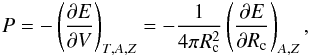 (A.1)where the volume V is identified with the volume Vc of the WS cell by treating the inner crust as a perfect crystal. With use of Leibniz’s rule for differentiation of a definite integral, the derivative of the energy (see Eq. (19)) with respect to the radius Rc of the WS cell is
 ![Mathematical equation: \appendix \setcounter{section}{1} \begin{eqnarray} \frac{\partial{E}}{\partial{ R_{\rm c}}} &=& 4{\pi} R_{\rm c}^{2} \Big[ {\cal H}\left(\rnum_{\rm n},\rnum_{\rm p}\right) + m_{\rm n}\rnum_{\rm n} + m_{\rm p}\rnum_{\rm p} + {\cal E}_{\rm el}\left(\rnum_{\rm e}\right) \nonumber \\[2mm] && \mbox{} + {\cal E}_{\rm coul}\left(\rnum_{\rm p},\rnum_{\rm e}\right) + {\cal E}_{\rm ex} \left(\rnum_{\rm p},\rnum_{\rm e}\right) \Big]_{r\,=\, R_{\rm c}} \nonumber \\[2mm] \label{eq17} && \mbox{} + 4{\pi}\int_{0}^{ R_{\rm c}}\left[\mu_{\rm n}\frac{\partial{\rnum_{\rm n}}}{\partial{ R_{\rm c}}} + \mu_{\rm p}\frac{\partial{\rnum_{\rm p}}}{\partial{ R_{\rm c}}} + \mu_{\rm e}\frac{\partial{\rnum_{\rm e}}}{\partial{ R_{\rm c}}}\right]r^{2}{\rm d}r. \end{eqnarray}](/articles/aa/full_html/2015/12/aa26642-15/aa26642-15-eq297.png) (A.2)For the calculation of the pressure this derivative is to be taken at constant mass and atomic numbers. If the neutron, proton, and electron numbers in the WS cell are fixed, we have
(A.2)For the calculation of the pressure this derivative is to be taken at constant mass and atomic numbers. If the neutron, proton, and electron numbers in the WS cell are fixed, we have 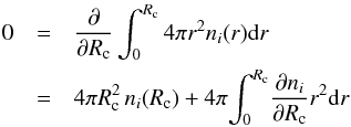 (A.3)for i = n,p,e, which in view of Eq. (A.2) allows writing
 ![Mathematical equation: \appendix \setcounter{section}{1} \begin{eqnarray} \left(\frac{\partial{E}}{\partial{ R_{\rm c}}}\right)_{A,Z} &=& 4{\pi} R_{\rm c}^{2} \Big[ {\cal H}\left(\rnum_{\rm n},\rnum_{\rm p}\right) + m_{\rm n}\rnum_{\rm n} + m_{\rm p}\rnum_{\rm p} + {\cal E}_{\rm el}\left(\rnum_{\rm e}\right) \nonumber \\[2mm] && \mbox{} + {\cal E}_{\rm coul}\left(\rnum_{\rm p},\rnum_{\rm e}\right) + {\cal E}_{\rm ex} \left(\rnum_{\rm p},\rnum_{\rm e}\right) \nonumber \\[2mm] \label{eq19} && \mbox{} -\mu_{\rm n}\rnum_{\rm n}-\mu_{\rm p}\rnum_{\rm p}-\mu_{\rm e}\rnum_{\rm e} \Big]_{r\,=\,R_{\rm c}}. \end{eqnarray}](/articles/aa/full_html/2015/12/aa26642-15/aa26642-15-eq300.png) (A.4)In the inner crust of a neutron star it is assumed that there are no protons in the gas of dripped neutrons and, consequently,
(A.4)In the inner crust of a neutron star it is assumed that there are no protons in the gas of dripped neutrons and, consequently,  . Therefore, at the edge of the cell we have
  ℋ(nn(Rc),0) and
 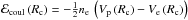 . Charge neutrality implies
  , because
  . Taking into account these constraints, it is easy to show that the nuclear contribution to the pressure is provided by only the interacting neutron gas at the edge of the WS cell. This neutron gas pressure is given by Png = μnnn(Rc) − [ℋ(nn(Rc),0) + mnnn(Rc)]. The variational Eq. (26) taken at r = Rc implies
 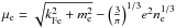 , and therefore the total pressure from the electrons is
 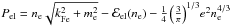 . We see that the free electron pressure is modified by the electronic Coulomb exchange by an amount (that is,
  , where
  is the contribution to the energy density due to electronic Coulomb exchange).
Putting together the previous results, Eq. (A.4) can be written as ![Mathematical equation: \appendix \setcounter{section}{1} \begin{eqnarray} \left(\frac{\partial{E}}{\partial{ R_{\rm c}}}\right)_{A,Z} = -4{\pi} R_{\rm c}^{2}\left[P_{\rm ng} + P_{\rm el}^{\rm free} + P_{\rm el}^{\rm ex}\right] . \label{eq20} \end{eqnarray}](/articles/aa/full_html/2015/12/aa26642-15/aa26642-15-eq313.png) (A.5)Thus, comparing with Eq. (A.1), we see that the pressure of the system takes the form
(A.5)Thus, comparing with Eq. (A.1), we see that the pressure of the system takes the form  , as stated in Sect. 4.
Appendix B: The minimization procedure in the inner crust revisited
As alluded to in Sect. 4, in this appendix we show explicitly that when the minimization of the energy per unit volume with respect to the radius Rc of the WS cell is attained, the Gibbs free energy per particle G/A equals the neutron chemical potential μn. For simplicity we restrict the derivation to the case of the spherical shape.
The optimal size Rc of the WS cell that minimizes the energy per unit volume under the constraints of a given average baryon density nb and charge neutrality is the solution of the equation ![Mathematical equation: \appendix \setcounter{section}{2} \begin{eqnarray} \frac{{\rm d}}{{\rm d} R_{\rm c}}\bigg[\frac{E}{V}\bigg] = \frac{1}{V}\bigg[-\frac{{\rm d}V}{{\rm d} R_{\rm c}} \frac{E}{V} + \frac{\partial E}{\partial R_{\rm c}}\bigg]=0, \label{eq23} \end{eqnarray}](/articles/aa/full_html/2015/12/aa26642-15/aa26642-15-eq316.png) (B.1)which results in the condition
(B.1)which results in the condition  (B.2)The total number of neutrons, protons, and electrons in the WS cell is given by
  (B.3)where xp is the proton fraction. Next we take the derivative of (B.3) with respect to Rc. We note that in the present calculation, where we are looking for the minimum of E/V vs. Rc, the number of neutrons and protons in the WS cell is not to be assumed fixed, and therefore Eq. (A.3) does not apply. From the derivative of (B.3) with respect to Rc, and recalling Leibniz’s rule for differentiation of integrals, one has
 ![Mathematical equation: \appendix \setcounter{section}{2} \begin{eqnarray} \label{eq25} &&4 \pi R_{\rm c}^2 \big[ \nb (1 - x_{\rm p}) - \rnum_{\rm n}( R_{\rm c}) \big] = 4 \pi \int^{ R_{\rm c}}_0 \frac{\partial{\rnum_{\rm n}(r)}}{{\partial R_{\rm c}}} r^2 {\rm d}r, \nonumber \\ &&4 \pi R_{\rm c}^2 \big[ \nb x_{\rm p} - \rnum_{\rm p}( R_{\rm c}) \big] = 4 \pi \int^{ R_{\rm c}}_0 \frac{\partial{\rnum_{\rm p}(r)}}{{\partial R_{\rm c}}} r^2 {\rm d}r, \nonumber \\ &&4 \pi R_{\rm c}^2 \big[ \nb x_{\rm p} - \rnum_{\rm e} \big] = 4 \pi \int^{ R_{\rm c}}_0 \frac{\partial{\rnum_{\rm e}}}{{\partial R_{\rm c}}} r^2 {\rm d}r. \end{eqnarray}](/articles/aa/full_html/2015/12/aa26642-15/aa26642-15-eq320.png) (B.4)The expression for ∂E/∂Rc has been given in Eq. (A.2). Using Eqs. (B.4) in (A.2) and taking into account that np(Rc) = 0 because there are no drip protons in the gas, one obtains
(B.4)The expression for ∂E/∂Rc has been given in Eq. (A.2). Using Eqs. (B.4) in (A.2) and taking into account that np(Rc) = 0 because there are no drip protons in the gas, one obtains ![Mathematical equation: \appendix \setcounter{section}{2} \begin{eqnarray} \frac{\partial{E}}{\partial{ R_{\rm c}}} &=& 4\pi R_{\rm c}^{2}\Big[{\cal H}\left(\rnum_{\rm n},0\right) + m_{\rm n}\rnum_{\rm n} + {\cal E}_{\rm el}\left(\rnum_{\rm e}\right) -\frac{3}{4}\left(\frac{3}{\pi}\right)^{1/3} \! \rnum_{\rm e}^{4/3} \nonumber \\[2mm] \label{eq26} && \mbox{} - \mu_{\rm n}\rnum_{\rm n} + \mu_{\rm n}\nb - \mu_{\rm e}\rnum_{\rm e} - \nb x_{\rm p} (\mu_{\rm n} - \mu_{\rm p} -\mu_{\rm e}) \Big]_{r\,=\, R_{\rm c}}. \nonumber \\[1mm] \end{eqnarray}](/articles/aa/full_html/2015/12/aa26642-15/aa26642-15-eq323.png) (B.5)Recalling that the pressure of the system is
(B.5)Recalling that the pressure of the system is  , the result (B.5) can be recast as
 ![Mathematical equation: \appendix \setcounter{section}{2} \begin{equation} \frac{\partial{E}}{\partial{ R_{\rm c}}} = 4{\pi} R_{\rm c}^{2} \left[- P + \mu_{\rm n} \nb - \nb x_{\rm p} (\mu_{\rm n} - \mu_{\rm p} - \mu_{\rm e}) \right]. \label{eq27} \end{equation}](/articles/aa/full_html/2015/12/aa26642-15/aa26642-15-eq325.png) (B.6)The minimization condition (B.2) implies
(B.6)The minimization condition (B.2) implies ![Mathematical equation: \appendix \setcounter{section}{2} \begin{equation} 4 \pi R_{\rm c}^2 \frac{E}{V} = 4{\pi} R_{\rm c}^{2}\left[- P + \mu_{\rm n} \nb - \nb x_{\rm p} (\mu_{\rm n} - \mu_{\rm p} - \mu_{\rm e}) \right], \label{eq28} \end{equation}](/articles/aa/full_html/2015/12/aa26642-15/aa26642-15-eq326.png) (B.7)and consequently,
(B.7)and consequently,  (B.8)When the system is in β-equilibrium, the chemical potentials fulfill μn − μp − μe = 0, and thus Eq. (B.8) gives
  (B.9)which confirms that at the minimum of the energy per unit volume with respect to the size of the cell, the Gibbs free energy equals the neutron chemical potential times the total number of baryons inside the WS cell.
All Tables
Properties of nuclear matter at saturation predicted by the EoS of this work in comparison with the empirical ranges (Newton et al. 2013; Steiner et al. 2010; Lattimer & Lim 2013; Hebeler et al. 2013; Chen et al. 2010; Tsang et al. 2012; Viñas et al. 2014).
Baryon density of the successive changes of energetically favourable topology in the inner crust.
All Figures
|
Fig. 1 Neutron (N) and proton (Z) numbers of the predicted nuclei in the outer crust of a neutron star using the experimental nuclear masses (Audi et al. 2012; Wolf et al. 2013) when available and the BCPM energy density functional or the FRDM mass formula (Möller et al. 1995) for the unmeasured masses. |
| In the text | |
|
Fig. 2 Pressure in the outer crust against baryon density using the experimental nuclear masses (Audi et al. 2012; Wolf et al. 2013) when available and the BCPM energy density functional or the FRDM mass formula (Möller et al. 1995) for the unmeasured masses. Also shown is the pressure from models BSk21, BPS, Lattimer-Swesty (LS-Ska), and Shen et al. (Shen-TM1) (see text for details). The dashed vertical line indicates the approximate end of the experimentally constrained region. |
| In the text | |
|
Fig. 3 Energy per baryon of different shapes relative to uniform npe matter as a function of baryon density in the inner crust. |
| In the text | |
|
Fig. 4 Energy per baryon of different shapes relative to uniform npe matter as a function of baryon density in the high-density region of the inner crust. |
| In the text | |
|
Fig. 5 The minimum energy per baryon relative to the neutron mass for different shapes as a function of the cell size Rc at an average baryon density nb = 0.077 fm-3. The value of the absolute minimum for each shape is shown in MeV in brackets. |
| In the text | |
|
Fig. 6 Radius Rc of the Wigner-Seitz cell and proton fraction xp = Z/A (given in percentage) in different geometries with respect to the baryon density. |
| In the text | |
|
Fig. 7 Mass number A (left vertical scale) and atomic number Z (right vertical scale) corresponding to spherical nuclei with respect to the baryon density. |
| In the text | |
|
Fig. 8 a) Optimal density profile of neutrons nn and protons np for spherical nuclear droplets at average baryon density nb = 0.0475 fm-3. The associated baryon and proton numbers, proton fraction xp = Z/A in percentage, and radius of the cell are shown. The vertical dashed line marks the location of the end of the WS cell. b) The same for nb = 0.065 fm-3. c) The same for nb = 0.076 fm-3. |
| In the text | |
|
Fig. 9 a) Optimal density profile of neutrons nn and protons np for rod shapes at average baryon density nb = 0.076 fm-3. The associated baryon and proton numbers, proton fraction xp = Z/A in percentage, and radius of the cell are shown. The vertical dashed line marks the location of the end of the WS cell. b) The same for slab shapes. c) The same for tube shapes. d) The same for bubble shapes. We note that the scale on the horizontal axis is the same in Figs. 9c and a, and in Figs. 9d and 8c. |
| In the text | |
|
Fig. 10 Energy per baryon relative to the neutron rest mass as a function of the average baryon density in the inner crust for the BCPM functional and other EoSs. |
| In the text | |
|
Fig. 11 Pressure as a function of the average baryon density in the inner crust for the BCPM functional and other EoSs. The figure starts at nb = 3 × 10⁻⁴ fm-3 where Fig. 2 ended. |
| In the text | |
|
Fig. 12 Adiabatic index from the EoSs of BCPM and DH-SLy4 (Douchin & Haensel 2001). The result calculated in homogeneous npe matter is also shown. |
| In the text | |
|
Fig. 13 Shear modulus from the EoS of BCPM and DH-SLy4 (Douchin & Haensel 2001). |
| In the text | |
|
Fig. 14 Populations vs. nucleon density for the BCPM EoS discussed in the text. The full red dot indicates the value of the nucleon density at which direct Urca processes set in. |
| In the text | |
|
Fig. 15 Pressure vs. nucleon density for the several EoSs discussed in the text, i.e. the BCPM (solid, red), the BSk21 (dot-dashed-dashed, magenta), the Lattimer-Swesty (Ska, dashed, blue), the Shen (dot-dashed, green), and the Douchin-Haensel (SLy4, dot-dot-dashed, black). A detail of the region between nb = 0.05 fm-3 and 0.30 fm-3 is shown in the inset. The incompressibility coefficients at nuclear saturation density for these models are K = 214 MeV (BCPM), 230 MeV (SLy4), 246 MeV (BSk21), 263 MeV (Ska), and 281 MeV (Shen). |
| In the text | |
|
Fig. 16 Gravitational mass, in units of the solar mass M⊙ = 2×1033 g vs. radius (left panel) and central density (right panel) in units of the saturation density n0 = 0.16 fm-3. See text for details. |
| In the text | |
|
Fig. 17 Density profiles for fixed mass configurations, i.e. MG = Mmax (solid blue curve), MG = 1.4 M⊙ (dashed red curve), and MG = 1.0 M⊙ (dot-dashed green curve). Full dots indicate the onset of the crust. In the inset the crust thickness is displayed for each fixed gravitational mass. See text for details. |
| In the text | |
Current usage metrics show cumulative count of Article Views (full-text article views including HTML views, PDF and ePub downloads, according to the available data) and Abstracts Views on Vision4Press platform.
Data correspond to usage on the plateform after 2015. The current usage metrics is available 48-96 hours after online publication and is updated daily on week days.
Initial download of the metrics may take a while.