| Issue |
A&A
Volume 583, November 2015
Rosetta mission results pre-perihelion
|
|
|---|---|---|
| Article Number | A40 | |
| Number of page(s) | 7 | |
| Section | Planets and planetary systems | |
| DOI | https://doi.org/10.1051/0004-6361/201526337 | |
| Published online | 30 October 2015 | |
CONSERT suggests a change in local properties of 67P/Churyumov-Gerasimenko’s nucleus at depth
1 UVSQ (UPSay), UPMC (Sorbonne Univ.), CNRS/INSU, LATMOS-IPSL, 78280 Guyancourt, France
e-mail: This email address is being protected from spambots. You need JavaScript enabled to view it.
2 UPMC (Sorbonne Univ.), UVSQ (UPSay), CNRS/INSU, LATMOS-IPSL, BC 102, 4 place Jussieu, 75005 Paris, France
3 Université de Toulouse, UPS-OMP, CNRS, IRAP, 9 avenue Colonel Roche, BP 44346, 31028 Toulouse Cedex 4, France
4 Technische Universität Dresden, 01069 Dresden, Germany
5 Université Grenoble Alpes, CNRS, IPAG, 38000 Grenoble, France
Received: 16 April 2015
Accepted: 29 June 2015
Abstract
Context. After the successful landing of Philae on the nucleus of 67P/Churyumov-Gerasimenko, the Rosetta mission provided the first opportunity of performing measurements with the CONSERT tomographic radar in November 2014. CONSERT data were acquired during this first science sequence. They unambiguously showed that propagation through the smaller lobe of the nucleus was achieved.
Aims. While the ultimate objective of the CONSERT radar is to perform the tomography of the nucleus, this paper focuses on the local characterization of the shallow subsurface in the area of Philae’s final landing site, specifically determining the possible presence of a permittivity gradient below the nucleus surface.
Methods. A number of electromagnetic simulations were made with a ray-tracing code to parametrically study how the gradient of the dielectric constant in the near-subsurface affects the ability of CONSERT to receive signals.
Results. At the 90 MHz frequency of CONSERT, the dielectric constant is a function of porosity, composition, and temperature. The dielectric constant values considered for the study are based on observations made by the other instruments of the Rosetta mission, which indicate a possible near-surface gradient in physical properties and on laboratory measurements made on analog samples.
Conclusions. The obtained simulated data clearly show that if the dielectric constant were increasing with depth, it would have prevented the reception of signal at the CONSERT location during the first science sequence. We conclude from our simulations that the dielectric constant most probably decreases with depth.
Key words: space vehicles: instruments / comets: individual: 67P/Churyumov-Gerasimenko / planets and satellites: formation / methods: numerical
© ESO, 2015
1. Introduction
The inner structure of cometary nuclei has never been systematically probed before ESA’s Rosetta rendezvous mission. Approaching the internal structure of cometary nuclei is crucial to better understand their formation in the early solar system and their subsequent evolution processes. The successful Rosetta mission with the recent descent and landing of Philae on the nucleus of 67P/Churyumov-Gerasimenko (hereafter 67P) in November 2014 has for the first time provided in situ data that are of the utmost importance in this matter.
The main scientific objective of the Comet Nucleus Sounding Experiment by Radiowave Transmission (CONSERT) radar is to sound the internal structure of the nucleus and provide first-hand information that will improve our understanding of the cometary formation and accretion processes. With receivers and transmitters onboard both Rosetta and Philae, the CONSERT bistatic radar uses radio waves at 90 MHz (with 10 MHz bandwidth) that have the ability to propagate through the nucleus between the main spacecraft and the lander (Kofman et al. 2007). The propagation of the electromagnetic waves is driven by the permittivity value inside the nucleus, more precisely, by the spatial variations of this value. Since we know that at the operating frequency of CONSERT, the permittivity depends on the porosity and on the composition of the nucleus and only to a lesser extent on temperature, data collected by CONSERT will provide information about these parameter values and their spatial variations inside the nucleus.
Here we specifically investigate the possible existence of a local subsurface permittivity gradient over depths ranging from tens to a few hundreds of meters. Even though the primary goal of CONSERT is to perform the tomography of the whole nucleus, the grazing angle configurations (where Rosetta is just below Philae’s horizon and where the propagation mainly takes place in the near surface zone) provide the best configurations from which to study the effect of a potential near-surface permittivity gradient beneath the lander (Ilyushin et al. 2003).
We here present results of simulations performed for a series of permittivity gradient values at grazing angle configurations that show the effect of such a gradient. We also offer a preliminary comparison with experimental data collected in the same Rosetta/Philae configuration.
2. Nucleus model
To produce simulated data for a comparison with experimental data collected by CONSERT, electromagnetic simulations were carried out with simple but realistic nucleus models. These were derived from our previous understanding of cometary nuclei that has been confirmed by the Rosetta mission for 67P.
2.1. 2D Nucleus shape and geometrical configuration
The nucleus shape model used for this work was derived from the images of the comet delivered by the Osiris camera on the Rosetta spacecraft. This is the preliminary DLR-SPG (based upon stereo-photogrammetry) CG SHAP4S shape model by the DLR-PF Rosetta 3D group, Berlin-Adlershof, 21-11-2014 (20141121_DLR_SPG_preliminarySHAP4S-4m-meshed_forCONSERT_fdynframe.obj).
Even if the Philae location is still not known with accuracy, triangulation performed with the delays measured with CONSERT have allowed narrowing down the uncertainty on its location (Kofman et al. 2015) to 20 m × 200 m. The work presented here assumes that Philae is located at the current best estimate of the actual Philae location at Abydos that is shown in Fig. 1 with a black dot on the 3D shape model of the nucleus.
Each colored dot in Fig. 1 represents the intersection of the straight line joining the Rosetta orbiter (≈15 km from the nucleus surface) to Philae with the surface of the 3D nucleus shape model for each sounding performed by CONSERT during the first science sequence (FSS). The green dots correspond to soundings that were performed for an orbiter location below the horizon that allowed the reception of clear signal.
Simulations performed on another location within the acceptable range of possible locations has been verified to not show any significant qualitative changes in the results.
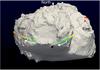 |
Fig. 1 Shape model of the nucleus. The colored dots show the intersection of the straight lines joining the Rosetta orbiter to the lander with the surface of the nucleus shape model. The black dot is the location of Philae. The green dots correspond to the soundings that were performed close to the grazing angle configuration used for the study. The white arrow shows the evolution with time of the sounding locations. |
Because of the nucleus rotation (with a period of about 12.4 h) combined with the motion of the Rosetta spacecraft, the dots corresponding to the soundings performed during the FSS do not belong to a single plane (see Fig. 1). Nevertheless, since we only consider the measurements performed at grazing angles (green dots), we can identify two different planes: one corresponding to the beginning of the FSS, west of the landing site (FSS-W), and another one corresponding to the end of the FSS, east of the landing site (FSS-E). These two planar slices of the 3D shape model are the basis for our 2D simulations; they are shown in Fig. 2. For both FSS-W and FSS-E, we work in Cartesian coordinate systems, with the assumed position of Philae at the origin, and north approximately toward the viewer. The orbiter location in these planes is given by the angle θ measured between the x-axis (indicated in the figure by an arrow) and the vector joining the locations of Philae and the orbiter. During FSS-W, the orbiter angular position θ in the 2D slice changed from −118.1° to −127.5° and from 80.3° and 105.8° during FSS-E.
 |
Fig. 2 2D configuration for FSS-W (top) and FSS-E (bottom). The slice of the comet is represented in color (red for the FSS-W – blue for FSS-E); north is approximately toward the viewer. The black dot shows the lander location. The successive locations of the orbiter during these sequences of the FSS are represented in black, and the dotted lines show the variations of the orbiter apparent angular locations (θ) for each of these sequences. |
2.2. Permittivity values
As already mentioned, the permittivity at the frequency of CONSERT is a function of porosities, compositions, and temperatures, both in the subsurface and inside the nucleus.
Bulk densities of cometary nuclei, as computed from their estimated volume, together with a tentative evaluation of their mass through nongravitational forces, have been estimated to remain in the range of 100 to 800 kg m-3 (e.g., Blum et al. 2006; Levasseur-Regourd et al. 2009). These expected values have now been validated for 67P, whose density is found from Rosetta data to be around 470 ± 45 kg m-3 (Sierks et al. 2015). The bulk porosity of the nucleus is thus quite high, ranging from 70 to 80% (Sierks et al. 2015). In agreement with the bulk density dependence derived from mixing formulae (Campbell & Ulrichs 1969), measurements on porous granular samples confirmed that, as expected, the dielectric constant value ϵ (which is the real part of the relative permittivity) systematically decreases with increasing porosity (Heggy et al. 2012; Brouet et al. 2014) with a typical slope value of about −4.7 × 10⁻² per percent at 90 MHz (Brouet et al. 2015).
Comets, as studied from previous flyby missions and remote spectroscopy, are composed of ices (mainly water ice) and refractory species, which consist of rock-forming elements (e.g., silicates) and of C, H, O, and N carbonaceous compounds (e.g., Cochran et al. 2015). The MIRO and VIRTIS experiments at 67P confirm these assumptions (e.g., Gulkis et al. 2015; Capaccioni et al. 2015). Consequently, the range of the permittivity values for the interior of the nucleus considered for our parametric study are those of porous and dirty water ice taken from Heggy et al. (2012) and Brouet et al. (2015), namely a dielectric constant ϵ ranging between 1.2 to 2.2. The imaginary part of the permittivity is expected to be low enough that it would only influence the amplitude of the received signal, which is not considered for the present study.
However, the external layer (up to a few meters) of the nucleus might have dielectric properties different from its interior. Nuclei typically have very low albedo values ranging from 0.03 to 0.06, indicating the presence of refractory materials (Lamy et al. 2004) in agreement with the fact that only limited patches of the surface are active icy regions. Indeed, VIRTIS, OSIRIS, and COSIMA observations during the second half of 2014 suggest that the nucleus of 67P is covered by an almost ice-free layer or mantle of dust particles (Capaccioni et al. 2015; Schulz et al. 2015; Thomas et al. 2015). For an ice-free and porous dust mantle at 300 K, the dielectric constant ϵ at the frequency of CONSERT is expected to be about two, decreasing from about 2.41 to 1.94 for porosities increasing from 70% to 80% (Brouet et al. 2015). However, the temperature at 67P during CONSERT measurements was significantly lower than 300 K: it was in the range of 180–230 K during daytime in VIRTIS surface measurements (Capaccioni et al. 2015) and in the range of 40–190 K in MIRO very shallow subsurface measurements (Gulkis et al. 2015). Laboratory measurements performed at low temperature on powered LL5 chondrite show a decrease in permittivity of about 25% for temperatures that decrease from 223 to 113 K (Heggy et al. 2001). For porosities increasing from 70% to 80%, an ice-free dust mantle at 110 K would have an ϵ decreasing from about 1.72 to 1.39, while a mantle with a dust-to-ice volumetric ratio equal to 1 would have a lower ϵ decreasing from about 1.65 to 1.33 (Brouet et al. 2015). Therefore, we can consider that a potential outer layer of the nucleus could have a dielectric constant value of about 1.5 ± 0.2.
Given the center frequency and frequency bandwidth of CONSERT, we do not expect to be able to detect any layer that would be thinner than 10 m or be sensitive to changes in permittivity that would occur at distances smaller than 3 m. We therefore considered for our simulations a potential variation with depth of the dielectric constant value that is described by a permittivity change Δϵ ranging from –0.5 to 0.5 that occurs over a thickness Δh from 10 m to 400 m below the surface. To consider a progressive transition between the outer layer and the interior of the nucleus, we chose to model the permittivity gradient by a half-cosine variation over the Δh thickness. While we are fully aware that the wave propagation simulated with such a permittivity model is model dependent, we nevertheless consider that the large-scale features and trends observed allow us to reach a generic conclusion.
3. Electromagnetic modeling
Our aim is to study by simulation the potential effect of the two parameters Δϵ and Δh on the CONSERT data and eventually to possibly constrain their values by the available CONSERT data. Computing the amplitude and delay of the signal received for each orbiter location would require a better knowledge of the lander position and attitude and of the orientation of its two antennas with respect to their close environment, which is not yet available. Consequently, the present work focuses on three main large-scale propagation behaviors that might occur because of refraction or reflection at the surface and/or inside an inhomogeneous nucleus: (i) there is direct visibility between orbiter and lander; (ii) no significant signal is received (occultation); (iii) several delayed replicas of the signal are received due to multipath propagation, disregarding the additional information that the knowledge of the amplitude and propagation delay of the received signals would provide.
3.1. Validation of the electromagnetic model used for the simulation
We performed a preliminary study with the aim to validate the electromagnetic model that was used to simulate the CONSERT data. To broadly study the effect of parameters Δϵ and Δh on the wave propagation through the nucleus, it is necessary to use a fast method for computing the received signal. A method capable of computing solutions for electromagnetic transfer through spatial dimensions much larger than the wavelength is the differential ray-tracing technique based on the Wentzel-Kramers-Brillouin (WKB) approximation. The applicability of this method is theoretically limited to small permittivity variations (Δϵ/ϵ< 10%) over a transition zone Δh that is significantly larger than the wavelength (≈3 m). Nevertheless, since we here only focus on identifying the large-scale propagation features mentioned above (disregarding amplitude and propagation delay values), we anticipated that the ray-tracing method might even be used for permittivity gradients that are too strong to be within the validity domain of the method.
The validity of applying the ray-tracing method for the limited CONSERT data analysis described above is shown by comparison with results obtained from the pseudo-spectral time-domain (PSTD) method. This method directly discretizes the Maxwell equations and simulates a time-domain solution in an iterative manner. The accuracy of this method is only determined by spatial and temporal step sizes and contains no other approximations; it yields accurate results.
For the purpose of this comparative study, the nucleus 2D slice was assumed to be a simple disk either homogeneous or with a permittivity gradient either positive or negative toward the center. While discrepancies could be noticed, as expected, between both electromagnetic models on the amplitudes computed and to a lesser extent on the calculated propagation delays, the receiver angular locations corresponding to each of the three propagation behaviors (visibility, occultation, multipath propagation) were similar for both methods.
We illustrate in Fig. 3 the comparison of the two simulation methods for the case of a dielectric constant value that varies from 1.5 to 2.5 within a layer 50 m thick beneath the nucleus surface. We note that given the dielectric constant variation considered here, the ray-tracing method is outside its validity domain. The propagation delay for each received signal was computed with both methods as a function of the orbiter angular position θ. In addition to the propagation delay, the color code used for the plot at the top of Fig. 3 displays the amplitude of the signals computed by the PSTD method; the signals that are too weak to be reasonably detected are displayed in yellow. While for this strong dielectric constant gradient, the ray-tracing method fails to correctly simulate the very weak signals of the PSTD method, neither method gives a signal or detectable signal for the very same θ values (approximately ranging from –45° and 45°, and for θ< −135° and θ> 45°), and consequently, the same angular extent for the occultation zone.
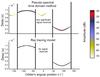 |
Fig. 3 Comparison of results obtained by simulation. The plot on the top of the figure has been obtained by the pseudo-spectral time-domain method while the one at the bottom shows the result of ray tracing simulations. Delays as a function of the orbiter’s angular position are plotted whenever a signal can be detected. The vertical lines highlight the angular positions of the orbiter that limit the area where no signal or only weak signal can be detected. |
Because the two methods give essentially the same results with respect to the geometry of signal propagation, we confidently used the ray-tracing method to identity for each (Δϵ, Δh) value of the orbiter angular positions where no signal can be detected.
3.2. Description of the simulated data products
Relying on its validity for our purpose, the ray-tracing method was intensively used to run a number of simulations for the previously defined nucleus dielectrical models and for the orbiter positions during FSS-E and FSS-W.
Figure 4 shows on the left an example of ray tracing that illustrates the three different behaviors due to refraction that have been mentioned above, namely: direct visibility, occultation, and multipath propagation. The nucleus model considered here has a permittivity value higher at depth than at the surface (Δϵ> 0). This kind of simulation allows one to estimate the number of rays arriving in a narrow (one degree) angular sector around any potential orbiter location, as shown in Fig. 5 right, and eventually to identify which of the three situations we have at a given orbiter location. The refraction phenomenon that is due to the permittivity gradient considered in Fig. 4 clearly leads to angular sectors (for θ values around –120° and 75°); labeled (ii), where no signal could be received by the orbiter. Logically, there are some values of the orbiter angular position θ; labeled (iii) (around –170° and 125°), where many rays would reach the receiver.
Figure 5 was obtained in a similar way, but this time, for a permittivity value lower at depth than at the surface (Δϵ> 0). The scales are the same as those used in Fig. 4 and allow an easy qualitative comparison. The rays here are not bent in the same away toward the interior of the nucleus, and as a consequence, the θ values corresponding to the absent signal are quite limited and even almost absent. This behavior is the basis for the study and analysis presented below.
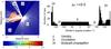 |
Fig. 4 Illustration of the data produced by the ray-tracing method and of the three different propagation behaviors. For this example, the permittivity value is higher at depth than at the surface (Δϵ> 0). Left: trajectories of rays propagating from the location of Philae. Right: numbers of rays arriving in an angular sector of 1 deg around the orbiter location as a function of the orbiter position θ. |
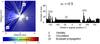 |
Fig. 5 Illustration of the data produced by the ray-tracing method and of the three different propagation behaviors (same as Fig. 4). For this example, the permittivity value is lower at depth than at the surface (Δϵ< 0). |
Sequences close to grazing angle where signal was received (UTC time and orbiter location).
The same analysis was performed systematically for a dielectric constant value of 1.7 at the surface and Δϵ values ranging from –0.5 to 0.5 and Δh values from 0.01 to 0.4 km. The purpose of the resulting parametric study is to quantify the effect of Δϵ and Δh with the aim to eventually use the information obtained from CONSERT to constrain the variation – if any – of permittivity with depth in the nucleus of 67P.
4. Results
4.1. Simulated data
The simulations described above were performed for orbiter angular positions that cover both FSS-E and FSS-W. Figures 6a (for the orbiter angular positions east of the landing site) and 6b (for the orbiter angular positions west of the landing site) summarize the results that were obtained in terms of numbers of rays at the receiver.
The dark blue areas correspond to configurations where no signal can be detected, the blue areas to a number of rays similar to what we obtain when the propagation occurs in vacuum, and the yellow or red areas to a number of rays significantly higher, which correspond to multipath propagation that is due to refraction. The ranges of orbiter angular positions for FSS-E and FSS-W are indicated in the figures. We note that the 2D slices of the nucleus that were used for the simulation are not relevant outside the FSS-E and FSS-W, where no conclusion should be drawn. These simulated data demonstrate that the two parameters Δϵ and Δh do have an impact on the angular extent and location of the occultation zones. The results obtained for the positions of the orbiter east (Fig. 6a) and west (Fig. 6b) of the lander show roughly symmetrical features, whose differences can be explained by the fact that the local radius of curvature of the nucleus surface is different for the eastern and western area of the landing site. Nevertheless, in both cases, a permittivity gradient would have had a noticeable effect on the ability of CONSERT to detect signal.
It is essential to remember that these simulated data were obtained for the half-cosine permittivity gradient model described above and that they are very likely to be model dependent. Nevertheless, the range of h values we used allowed us to investigate the effect of a variety of gradients, from those that change slowly to those that change abruptly, and we are confident that any other model for the permittivity gradient would have induced the same behavior. Consequently, we can safely exclude any increase of permittivity with depth for the small lobe of the nucleus that has been sounded by CONSERT during FSS.
Observations made by the other instruments of the Rosetta mission indicate that the nucleus is covered by a mantle that certainly has dielectric properties different from the ones at depth (Schloerb et al. 2015), which would be consistent with an inhomogeneous nucleus. Nevertheless, it is impossible for the moment to exclude the hypothesis of a homogeneous nucleus below a mantle too thin to have a sensible effect on CONSERT’s measurements. Therefore, we performed a supplementary study for homogeneous nuclei for dielectric constant values ranging from 1.2 to 2.2. The results are shown in Figs. 7a (for the orbiter angular positions east of the landing site) and 7b (for the orbiter angular positions west of the landing site). We see that the areas without signal (the dark ones) are larger for higher dielectric constant values. This effect is more visible in Fig. 7b because the local radius curves at the surface west of the landing site.
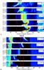 |
Fig. 6 Numbers of rays received as a function of the orbiter location and Δh values for five different values of Δϵ. The location of the orbiter is east of the landing site for a) and west for b). The configurations leading to no signal are shown in dark blue; those corresponding to a high number of rays (multipath scenario) are plotted in yellow and red. The vertical red lines show the angular positions of the orbiter during FSS-E and FSS-W. |
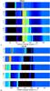 |
Fig. 7 Numbers of rays received as a function of the orbiter location for a homogeneous nucleus. Five different values of ϵ have been considered. The location of the orbiter is east of the landing site for a) and west for b). The configurations leading to no signal are shown in dark blue; those corresponding to a high number of rays (multipath scenario) are plotted in yellow and red. The vertical red lines show the angular positions of the orbiter during FSS-E and FSS-W. |
4.2. Qualitative comparison with CONSERT data and discussion
Even if the orbit configuration resulting from the final landing site location did not allow us to perform any measurement in visibility that could have been used as reference, the measurements that were performed show that signal was clearly received (Kofman et al. 2015) throughout both FSS-W and FSS-E. Given the geometrical configurations during these two sequences of the FSS, only the sounding of the smaller lobe of the cometary nucleus was possible then. Therefore, the study presented here cannot provide any information about the permittivity inside the larger lobe of the nucleus.
As explained previously, we consider neither the amplitude nor the propagation delay of the received signals. Instead, we exclusively used the fact that signals were actually received during FSS-E and FSS-W (see Table 1). Relying on the simulation results displayed in Sect. 4.1, we can thus exclude (Δϵ, Δh) combinations that would result in an occultation situation during FSS-W and/or FSS-E.
Since the dark blue areas of Fig. 6 correspond to configurations where no significant signal can be received, we conclude that for both series of measurements (FSS-E and FSS-W), a value of Δϵ> 0 (permittivity higher at depth than at the surface) would have prevented any signal detection by CONSERT and must therefore be excluded.
A more detailed analysis of the results for FSS-E shows that for Δϵ ≈ −0.4, h values ranging from 125 to 175 m show no dark zones at all for the whole angular extent of FSS-E and are thus most likely to be compatible with the CONSERT data acquired during this measurement sequence. On the other hand, the same analysis for FSS-W would be in favor of a Δϵ = −0.4 with Δh values ranging from 150 m to 250 m. At this stage, it is impossible to conclude more precisely on a potential difference that might be existing in the near subsurface between the two regions east and west of the location of Philae without taking into account additional information such as the measured propagation delays. According to the study, the most consistent values for the dielectric constant are about 1.7 at the surface and 1.3 at depth and would occur over a distance on the order of 150 m.
This decrease in permittivity with depth can be explained by an increased porosity and/or a decrease in the dust-to-ice ratio at depth. Based on the findings that at the comet surface the dust/ice ratio is around 4 (Rotundi et al. 2015), the average porosity is around 70–80% (Sierks et al. 2015), and the temperature below the surface is between 40 K and 190 K (Gulkis et al. 2015), the Δϵ value of –0.4 can be interpreted as a increase in porosity with depth of 15% for a temperature around 110K (Brouet et al. 2015) or as a decrease in the dust-to-ice ratio from 4 to 0.1 at 153 K (Heggy et al. 2012). We note that a significantly higher temperature inside the nucleus would require a much lower variation of the dust-to-ice ratio. At 193 K, for instance, a dust-to-ice ratio of around 0.5 would be sufficient to explain the Δϵ value of –0.4. Seeing that the VIRTIS instrument detected no pure ice on the surface of the comet (Capaccioni et al. 2015), a combination of these effects is likely in order to generate the gradient in dielectric constant we estimated. The change most likely occurs over a thickness of about one hundred meters.
The analysis of the results obtained for a hypothetical homogeneous nucleus (see Fig. 7) shows that the refraction induced by a dielectric constant value ≥1.45 inside the comet would have prevented the propagation of the waves between the lander and the orbiter locations during FSS-W (Fig. 7b). The result for FSS-E (Fig. 7a) is less definite, but we can assume that any ϵ value higher than 1.7 is inconsistent with the signal actually received during the whole FSS-E. Additional simulation runs for ϵ values between 1.2 and 1.45 show that the highest acceptable value for the whole FSS would be 1.35. It therefore seems reasonably safe to conclude that in the hypothesis of a homogeneous nucleus, the dielectric constant value would be lower than 1.35, consistent with a 80% porosity and a dust-to-ice ratio lower than 1.5 (Brouet et al. 2015). This value is consistent with the average value of about 1.27 that has been estimated by Kofman et al. (2015) after a study performed on a homogeneous nucleus and based on the propagation delays measured by CONSERT.
5. Conclusions
During the first science sequence, when the Rosetta orbiter was just below the Philae lander horizon, the electromagnetic waves transmitted by the lander were able to propagate through the small lobe of the nucleus and to eventually reach the orbiter. Our results here are based on this. Assuming that the nucleus is not homogeneous, we obtained an estimate of the dielectric constant gradient below the surface of the comet. Our best estimate, which is consistent with the observations made at the surface and the bulk properties of the nucleus, is that the dielectric constant decreases with depth from about 1.7 at the surface to about 1.3 over a thickness of about one hundred meters. The parametric study performed with our simulations give us confidence that even if the quantitative values are not narrowly constrained, the trend is significant.
Based on laboratory measurements made at low temperature on porous dirty ice samples, we suggest that this variation might be due to a decrease in the dust-to-ice content at depth or to an increase in porosity with depth, consistent with current measurements made by Rosetta.
Future observations made by the instruments of the Rosetta payload when the comet becomes more and more active will provide additional information on the nucleus properties at depth, which we will use to refine our analysis.
Whenever the exact location of Philae and the orientation of the CONSERT antennas with respect to their close environment are available, it will be possible to perform a supplementary study that may better constrain the amplitudes and the internal structure of the nucleus.
Acknowledgments
Rosetta is an ESA Cornerstone Mission. Philae is a DLR/CNES lander. The research on the CONSERT experiment is supported by funding from the Centre National d’Études Spatiales (CNES) and the Deutsches Zentrum für Luft- und Raumfahrt (DLR). CONSERT is a bistatic radar, between the lander and the orbiter, dedicated to the tomography of the deep interior of the comet nucleus. CONSERT was designed and built by a consortium led by IPAG UJF/CNRS (France), in collaboration with LATMOS (France) and MPS Gottingen (Germany). The authors thank Holger Sierks (Max-Planck-Institut für Sonnensystemforschung), Laurent Jorda (Laboratoire d’Astrophysique de Marseille) and Frank Preusker (German Aerospace Center - DLR) for the nucleus shape model used in this paper (20141121_DLR_SPG_preliminarySHAP4S-4m-meshed_forCONSERT_fdynframe.obj).
References
- Blum, J., Schräpler, R., Davidsson, B. J., & Trigo-Rodríguez, J. M. 2006, ApJ, 652, 1768 [NASA ADS] [CrossRef] [Google Scholar]
- Brouet, Y., Levasseur-Regourd, A. C., Encrenaz, P., & Gulkis, S. 2014, Planet. Space Sci., 103, 143 [NASA ADS] [CrossRef] [Google Scholar]
- Brouet, Y., Levasseur-Regourd, A. C., Sabouroux, P., et al. 2015, A&A, 583, A39 [NASA ADS] [CrossRef] [EDP Sciences] [Google Scholar]
- Campbell, M. J., & Ulrichs, J. 1969, J. Geophys. Res., 74, 5867 [NASA ADS] [CrossRef] [Google Scholar]
- Capaccioni, F., Coradini, A., Filacchione, G., et al. 2015, Science, 347, 0628 [NASA ADS] [CrossRef] [Google Scholar]
- Cochran, A. L., Levasseur-Regourd, A. C., Cordiner, M., et al. 2015, Space Sci. Rev., submitted [Google Scholar]
- Gulkis, S., Allen, M., von Allmen, P., et al. 2015, Science, 347, 0709 [Google Scholar]
- Heggy, E., Paillou, P., Ruffié, G., et al. 2001, Icarus, 154, 244 [NASA ADS] [CrossRef] [Google Scholar]
- Heggy, E., Palmer, E. M., Kofman, W., et al. 2012, Icarus, 221, 925 [NASA ADS] [CrossRef] [Google Scholar]
- Ilyushin, Y., Hagfors, T., & Kunitsyn, V. 2003, Radio Science, 38, 8 [NASA ADS] [CrossRef] [Google Scholar]
- Kofman, W., Hérique, A., Goutail, J.-P., et al. 2007, Space Sci. Rev., 128, 413 [NASA ADS] [CrossRef] [Google Scholar]
- Kofman, W., Hérique, A., Barbin, Y., et al. 2015, Science, 349, 6247 [CrossRef] [Google Scholar]
- Lamy, P. L., Toth, I., Fernandez, Y. R., & Weaver, H. A. 2004, in Comets II, eds. M. C. Festou, H. U. Keller, & H. A. Weaver (Univ. Arizona Press), 223 [Google Scholar]
- Levasseur-Regourd, A. C., Hadamcik, E., Desvoivres, E., & Lasue, J. 2009,Planet. Space Sci., 57, 221 [Google Scholar]
- Rotundi, A., Sierks, H., Della Corte, V., et al. 2015, Science, 347, 3905 [Google Scholar]
- Schloerb, F. P., Keihm, S., von Allmen, P., et al. 2015, A&A, 583, A29 [NASA ADS] [CrossRef] [EDP Sciences] [Google Scholar]
- Schulz, R., Hilchenbach, M., Langevin, Y., et al. 2015, Nature, 518, 216 [NASA ADS] [CrossRef] [Google Scholar]
- Sierks, H., Barbieri, C., Lamy, P. L., et al. 2015, Science, 347, 1044 [NASA ADS] [CrossRef] [Google Scholar]
- Thomas, N., Sierks, H., Barbieri, C., et al. 2015, Science, 347, 0440 [CrossRef] [Google Scholar]
All Tables
Sequences close to grazing angle where signal was received (UTC time and orbiter location).
All Figures
|
Fig. 1 Shape model of the nucleus. The colored dots show the intersection of the straight lines joining the Rosetta orbiter to the lander with the surface of the nucleus shape model. The black dot is the location of Philae. The green dots correspond to the soundings that were performed close to the grazing angle configuration used for the study. The white arrow shows the evolution with time of the sounding locations. |
| In the text | |
|
Fig. 2 2D configuration for FSS-W (top) and FSS-E (bottom). The slice of the comet is represented in color (red for the FSS-W – blue for FSS-E); north is approximately toward the viewer. The black dot shows the lander location. The successive locations of the orbiter during these sequences of the FSS are represented in black, and the dotted lines show the variations of the orbiter apparent angular locations (θ) for each of these sequences. |
| In the text | |
|
Fig. 3 Comparison of results obtained by simulation. The plot on the top of the figure has been obtained by the pseudo-spectral time-domain method while the one at the bottom shows the result of ray tracing simulations. Delays as a function of the orbiter’s angular position are plotted whenever a signal can be detected. The vertical lines highlight the angular positions of the orbiter that limit the area where no signal or only weak signal can be detected. |
| In the text | |
|
Fig. 4 Illustration of the data produced by the ray-tracing method and of the three different propagation behaviors. For this example, the permittivity value is higher at depth than at the surface (Δϵ> 0). Left: trajectories of rays propagating from the location of Philae. Right: numbers of rays arriving in an angular sector of 1 deg around the orbiter location as a function of the orbiter position θ. |
| In the text | |
|
Fig. 5 Illustration of the data produced by the ray-tracing method and of the three different propagation behaviors (same as Fig. 4). For this example, the permittivity value is lower at depth than at the surface (Δϵ< 0). |
| In the text | |
|
Fig. 6 Numbers of rays received as a function of the orbiter location and Δh values for five different values of Δϵ. The location of the orbiter is east of the landing site for a) and west for b). The configurations leading to no signal are shown in dark blue; those corresponding to a high number of rays (multipath scenario) are plotted in yellow and red. The vertical red lines show the angular positions of the orbiter during FSS-E and FSS-W. |
| In the text | |
|
Fig. 7 Numbers of rays received as a function of the orbiter location for a homogeneous nucleus. Five different values of ϵ have been considered. The location of the orbiter is east of the landing site for a) and west for b). The configurations leading to no signal are shown in dark blue; those corresponding to a high number of rays (multipath scenario) are plotted in yellow and red. The vertical red lines show the angular positions of the orbiter during FSS-E and FSS-W. |
| In the text | |
Current usage metrics show cumulative count of Article Views (full-text article views including HTML views, PDF and ePub downloads, according to the available data) and Abstracts Views on Vision4Press platform.
Data correspond to usage on the plateform after 2015. The current usage metrics is available 48-96 hours after online publication and is updated daily on week days.
Initial download of the metrics may take a while.