| Issue |
A&A
Volume 583, November 2015
|
|
|---|---|---|
| Article Number | A122 | |
| Number of page(s) | 11 | |
| Section | Catalogs and data | |
| DOI | https://doi.org/10.1051/0004-6361/201425503 | |
| Published online | 04 November 2015 | |
The variability behaviour of CoRoT M-giant stars⋆,⋆⋆
1 Departamento de Física, Universidade Federal do Rio Grande do Norte, RN, 59072-970, Natal, Brazil
e-mail: This email address is being protected from spambots. You need JavaScript enabled to view it.
2 SUPA (Scottish Universities Physics Alliance) Wide-Field Astronomy Unit, Institute for Astronomy, School of Physics and Astronomy, University of Edinburgh, Royal Observatory, Blackford Hill, Edinburgh EH9 3HJ, UK
3 LESIA, UMR 8109 CNRS, Observatoire de Paris, UVSQ, Université Paris-Diderot, 5 place J. Janssen, 92195 Meudon, France
4 Universidade de São Paulo/IAG-USP, rua do Matão, 1226, Cidade Universitária, SP, 05508-900, São Paulo, Brazil
Received: 11 December 2014
Accepted: 8 August 2015
Abstract
Context. For six years the Convection, Rotation, and planetary Transits (CoRoT) space mission has been acquiring photometric data from more than 100 000 point sources towards and directly opposite the inner and outer regions of the Galaxy. The high temporal resolution of the CoRoT data, combined with the wide time span of the observations, enabled the study of short- and long-time variations in unprecedented detail.
Aims. The aim of this work is to study the variability and evolutionary behaviour of M-giant stars using CoRot data.
Methods. From the initial sample of 2534 stars classified as M giants in the CoRoT databases, we selected 1428 targets that exhibit well defined variability, by visual inspection. Then, we defined three catalogues: C1 – stars with Teff< 4200 K and LCs displaying semi-sinusoidal signatures; C2 – rotating variable candidates with Teff> 4200 K; C3 – long-period variable candidates (with LCs showing a variability period up to the total time span of the observations). The variability period and amplitude of C1 stars were computed using Lomb-Scargle and harmonic fit methods. Finally, we used C1 and C3 stars to study the variability behaviour of M-giant stars.
Results. The trends found in the V−I vs. J−K colour–colour diagram are in agreement with standard empirical calibrations for M giants. The sources located towards the inner regions of the Galaxy are distributed throughout the diagram, while the majority of the stars towards the outer regions of the Galaxy are spread between the calibrations of M giants and the predicted position for carbon stars. The stars classified as supergiants follow a different sequence from the one found for giant stars. We also performed a Kolmogorov-Smirnov (KS) test of the period and amplitude of stars towards the inner and outer regions of the Galaxy. We obtained a low probability that the two samples came from the same parent distribution. The observed behaviour of the period-amplitude and period-effective temperature (Teff) diagrams are, in general, in agreement with those found for Kepler sources and ground based photometry, with pulsation being the dominant cause responsible for the observed modulation. We also conclude that short-time variations on M-giant stars do not exist or are very rare, and the few cases we found are possibly related to biases or background stars.
Key words: catalogs / stars: oscillations / stars: evolution
The CoRoT space mission was developed and is operated by the French space agency CNES, with the participation of ESA’s RSSD and Science Programmes, Austria, Belgium, Brazil, Germany, and Spain.
Full Tables 2–4 are only available at the CDS via anonymous ftp to cdsarc.u-strasbg.fr (130.79.128.5) or via http://cdsarc.u-strasbg.fr/viz-bin/qcat?J/A+A/583/A122
© ESO, 2015
1. Introduction
The Convection, Rotation, and planetary Transits (CoRoT; Baglin et al. 2007) and Kepler (Borucki et al. 2010) photometry space missions have enabled us to improve our knowledge of a large variety of stellar phenomena, such as the rotational behaviour of different families of stars (e.g., Affer et al. 2012; De Medeiros et al. 2013; Nielsen et al. 2013; McQuillan et al. 2013; de Freitas et al. 2013), detection and characterisation of a wide variety of extrasolar planets (e.g., Léger et al. 2009; Borucki et al. 2012; Batalha et al. 2013), and their host stars (e.g., Brown et al. 2011; Dressing & Charbonneau 2013; Morton & Swift 2014; Huber et al. 2014), the analysis of stellar interiors using asteroseismology (e.g., Huber et al. 2012; Silva Aguirre et al. 2012; Hekker et al. 2013), characterisation of surface differential rotation (Lanza et al. 2014), and the detection of eclipsing binary systems (e.g., Maceroni et al. 2009; Slawson et al. 2011; Maciel et al. 2011). The aforementioned science cases represent only a few of the major topics among the many aspects of time-domain, high-precision photometry. The data provided by the CoRoT and Kepler space missions represent the most complete dataset for the study of stellar variability available to date (e.g., De Medeiros et al. 2013; Walkowicz & Basri 2013). In general the results from each mission agree with each other, but there is a lack of a comparative study of M-type stars.
One of the fundamental questions in debate in the literature is the evolution and nature of the pulsations in M giants. Our recent understanding of how M giants oscillate was obtained from ground-based surveys such as MACHO, OGLE, and EROS (e.g., Wood & Sebo 1996; Alard et al. 2001; Lebzelter et al. 2002; Kiss & Bedding 2003; Soszynski et al. 2007; Riebel et al. 2010; Wiśniewski et al. 2011; Soszyński et al. 2013), as well as solar neighbourhood observations (Tabur et al. 2010).
Another important question concerns the evolution and nature of the pulsations in the GK-M type giant transition in the red giant branch (RGB). Whether the main physical mechanism of the pulsations of M giants is self-excited (Mira-type) pulsations or stochastic (solar-type) oscillations is still not clear (e.g., Dziembowski et al. 2001; Christensen-Dalsgaard et al. 2001; Bedding et al. 2005).
In this context, Tabur et al. (2010) show that, as we advance through the RGB, the observed low amplitude of stochastically excited solar-type oscillations, which is typical of the GK-type giants, progress to a mixture of Mira-like and solar-like variability, as found in semi-regular (SR) variables, and ending with stable, mono-periodic, Mira-like pulsations. Afterwards, Mosser et al. (2013) studied global oscillation parameters of Kepler red giants, concluding that the main excitation mechanism in M giant SR variables are solar-like oscillations, thus confirming the findings of Dziembowski & Soszyński (2010), but they were unable to disentangle RGB from AGB stars. In this regard, Stello et al. (2014) detected non-radial modes in early M giants, as previously found by Mosser et al. (2013) for less luminous giants. Bányai et al. (2013) performed a detailed study of the variability of M-type giants using Kepler data as well. They affirm that they could distinguish between solar-like oscillations and larger amplitude pulsations. They found a correlation of solar-like oscillations with period that closely follows the well-known vmax amplitude scaling relations (e.g., Mosser et al. 2010, 2013; Huber et al. 2011), but they found a sharp ending to this correlation at log P ~ 1. This feature may be an indication that a different excitation mechanism dominates from this point on. Does this point mark the transition between solar-like and Mira-type pulsations? In their diagram, the stars classified as having a few periodic components (Miras and SRs) then follow a trend with a steeper slope for log P greater than 1. This trend is similar to the one found by Tabur et al. (2010) for bright M-giant stars, which depicts overtone pulsators, with a few stars following the fundamental mode trend (typical of Mira-type stars) as well.
Another point of discussion concerns the observation of rapid variations in brightness on timescales between three minutes to 30 days in long-period variables (LPVs; e.g., Schaefer 1991; Maffei & Tosti 1995; de Laverny et al. 1998). However, these events have not been confirmed in recent studies (e.g., Mais et al. 2004; Woźniak et al. 2004; Lebzelter 2011; Hartig et al. 2014). Indeed, using data from CoRoT and Kepler, Lebzelter (2011) and Hartig et al. (2014) do not confirm such variations, despite photometric precisions of a few mmag. Therefore, the observed short-time variations are very rare or not physical.
In this study we comprehensively analyse the variability of M giants observed by CoRoT, and we compare our results with previous studies of the variability behaviour of M giant stars observed by other authors. The paper is structured as follows. In Sect. 2, we describe our working sample and our catalogue. In Sect. 3, we present our results and compare them with previous works from the literature. We also investigate the difference between CoRoT stars located towards the inner and outer regions of the Galaxy. Finally, in Sect. 4, we present our conclusions and discuss future perspectives.
2. Working sample
The CoRoT satellite was launched in 2006. It collected point-source photometric data towards inner (around RA = 18h50m, Dec = +00) and outer (around RA = 06h50m, Dec = +00) regions of the Galaxy over a period of six years. A total of 162 789 sources were observed, with 5762 classified as M-type stars (Deleuil et al. 2009). These stars constitute approximately 4% of all stars observed by CoRoT and are divided in two main groups: giants (luminosity classes I–III) and dwarfs (luminosity class V). Giants comprise approximately 44% of all M-type stars detected by CoRoT, whereas the percentage of M dwarfs is approximately 56%. A total of 973 M-type stars were observed at least twice, providing a unique sample for studying long-term photometric variations. Table 1 lists the number of M-type stars observed with CoRoT towards the inner (centre) and outer (anticentre) regions of the Galaxy.
CoRoT M-type stars taken from EXO-Dat (Deleuil et al. 2009) distributed by luminosity class.
The latest CoRoT data release N21 provides light curves (LCs) that are corrected for instrumental noise caused by electronic, background, and jitter sources. The effect of the South Atlantic Anomaly (SAA) passage was also included, and hot pixels of the detector are now flagged (Auvergne et al. 2009). When beginning this work, the data were not yet completely corrected and some problems remained in the released data, requiring further treatment before the data was ready for analysis. In particular, the data contained long-term trends produced by CCD temperature variations, jumps (discontinuities) produced by hot pixels, and outliers (Auvergne et al. 2009). The post-processing of the LCs performed in different works follows different methods, according to the objectives of the works (e.g., Renner et al. 2008; Basri et al. 2011; Affer et al. 2012; De Medeiros et al. 2013), and to date, no standard method exists for analysing the processed data. In this work, we follow the general guidelines presented by De Medeiros et al. (2013).
First, we selected all sources classified as M-type giant stars in the CoRoT database. This first pre-selection, which yielded 2534 objects, provided us with a reasonable quantity of actual giants, although the luminosity class specified in the CoRoT database is sometimes incorrect.
We also obtained the Harris V and Sloan-Gunn r′ and i′ photometry from the Exo-Dat database (Deleuil et al. 2009) and JHKs photometry from the Two Micron All Sky Survey (2MASS- Skrutskie et al. 2006) catalogue. The indexes V, r′, and i′ were transformed into Johnson V- and I-band photometry using the relations in Deleuil et al. (2009) with propagation of the respective errors.
Then, we derredened the photometry using the extinction coefficients AV, AI, AJ, and AK that were calculated with the relations from Schlafly & Finkbeiner (2011) and E(B−V) reddening maps taken from Schlafly et al. (2014). We took the uncertainties from the coefficients and reddening maps and propagated them to obtain the final uncertainty of the corrected photometry. The transformed Johnson photometry and the unreddened photometry are listed in Tables 2–4.
Stellar parameters of C1 for the first 10 stars.
Stellar parameters of C2 for the first 10 stars.
Stellar parameters of C3 for the first 10 stars.
2.1. Cross-identification
We performed a systematic cross-check of the 2534 M giants to identify previous studies in the literature. To this end, we used the SIMBAD database2, the General Catalogue of Variable Stars (Samus et al. 2009), the AAVSO International Variable Star Index (VSX v1.1, which now includes 325 346 variable stars – Watson et al. 2014), the New Catalogue of Suspected Variable Stars (Kazarovets et al. 1998), the Northern Sky Variability Survey catalogue (NSVS – Hoffman et al. 2009), and a few catalogues of carbon stars (MacConnell 1988; Stephenson 1989, 1996; Alksnis et al. 2001; Chen & Yang 2012; Zacharias et al. 2013). We also cross-checked with previous studies using CoRoT data (Lebzelter 2011; Sebastian et al. 2012; Guenther et al. 2012; Sarro et al. 2013; De Medeiros et al. 2013). Finally, we also searched in many other databases incorporated in the International Virtual Observatory Alliance3, using the Tool for OPerations on Catalogues And Tables (TOPCAT4 – Taylor 2005). The search achieved a positional accuracy of 2′′ in the sky coordinates.
We found a total of 465 stars in common with other studies. Among these there are 390 semi-sinusoidal variables, 45 LPVs, 14 Orion-type variable stars, eight carbon stars, six Mira-type stars, four binary systems, two pre-main sequence stars, two high proper-motion stars, one δ Scuti star, and one γ Doradus star. Some of these stars have more than one classification. For instance, 15 semi-sinusoidal variables are also classified as LPVs. At the same time, not every star has a known period. The Orion type, γ Doradus, and pre-main sequence stars, as well as stars in binary systems, were eliminated from our sample. The remaining sources were used to compare our period measurements (see Sect. 2.3). The stars in common with the literature that depict their variability types are presented in Col. 2 of Tables 2 and 3).
2.2. Effective temperature estimation
The Teff values of the M giants were calculated using the photometric-effective temperature relation of van Belle et al. (1999),  (1)This procedure was chosen to provide a homogeneous set of Teff estimations. This is a precise tool directly based on interferometric measurements.
The effective temperature was calculated using the unreddened V- and KS-band photometry. We transformed the KS magnitudes to KCIT photometry using the relation of Carpenter (2001) and calculated the Teff values. The KCIT photometry was used because it is the closest band to the one that was used to establish the original calibration (van Belle, priv. comm.).
The uncertainties in the Teff values were estimated by propagating the errors of the corrected magnitudes and the KS transformation uncertainty. Then, we added the photometric uncertainty in quadrature to the estimated errors from Table 8 of van Belle et al. (1999), taking the maximum error of the two V−K bins that were closest to each parameter value. The results are presented in Tables 2–4.
2.3. Variability analysis
A Lomb-Scargle periodogram (Lomb 1976; Scargle 1982) was computed for each LC, except for the LPV candidates (C3 – see Sect. 2.4). We set the low-frequency limit (f0) for each periodogram to f0 = 1 /Ttot, where Ttot is the total time spanned by the LC. The high-frequency limit was fixed to fN = 10 d-1, and the periodogram size was scaled to 104 elements. The highest periodogram peak, which is referred to as frequency f1 or period P1, was refined following De Medeiros et al. (2013), namely, by maximizing the ratio of the variability amplitude to the minimum dispersion given by Dworetsky (1983). Next, the refined frequency f1 was used to calculate a harmonic fit with two harmonics. This fit was used as a model to compute the mean variability amplitude (A) in units of magnitude (mag), and is defined as ![Mathematical equation: \begin{equation} y(t) = \sum_{j \, =\, 1}^{2}\left[a_{j}\sin\left(2\pi f_{1} j t \right) + b_{j}\cos\left(2\pi f_{1} j t \right) \right] + b_0, \label{eq_best_harm} \end{equation}](/articles/aa/full_html/2015/11/aa25503-14/aa25503-14-eq48.png) (2)in the phase diagram of the main period, where f1 is the frequency, aj and bj are the Fourier coefficients, t is the time, and b0 is the background level.
(2)in the phase diagram of the main period, where f1 is the frequency, aj and bj are the Fourier coefficients, t is the time, and b0 is the background level.
For our M giants (typically stars with Teff< 4200 K – see Sect. 2.4), we defined the variability amplitude as half of the difference between the maximum and minimum of Eq. (2) in the phase diagram of the main period, which is similar to the amplitude definitions used by De Medeiros et al. (2013) and Bányai et al. (2013). This fit was then applied to the LC domain and was subtracted from the time series (pre-whitening), thereby yielding a new Lomb-Scargle periodogram. The procedure was iterated N times; in each iteration, the LCs were fitted with a harmonic fit using two harmonics. For each LC, we selected all the independent periods that exhibited a significance level greater than 99%, i.e., a false alarm probability (FAP) less than 0.01. Therefore, a collective set of independent periods for each target was retained to perform an analysis that was similar to that of Tabur et al. (2010) and Bányai et al. (2013), where we retained the first three periods above the FAP, as shown in Table 2. The FAP was computed based on the Eaton et al. (1995) method, which consists of randomising the temporal bins of the original LC and computing the resulting power spectra (see also Affer et al. 2012). We produced 1000 modified LCs for each period by randomising the positions of blocks of adjacent temporal bins, with a block length of 12 h, in accordance with Affer et al. (2012). Regarding our semi-sinusoidal sources with Teff> 4200 K (C2 – see Sect. 2.4), we performed the analysis once and kept only one period and amplitude (see Table 3).
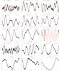 |
Fig. 1 Typical LCs of stars from our catalogue. CoRoT-ID and period of the C1 (row 1–3) and C2 (row 4) catalogues are shown in the headers. For the C3 (LPVs – row 5) sources, only the CoRoT-ID is shown. The red line indicates the harmonic fit models of the C1 stars given by Eq. (2). |
A total of 434 stars were found with previously determined periods (Lebzelter 2011; De Medeiros et al. 2013). For approximately 96% of the targets, the differences between our periods and those periods of the other authors are less than 10%. We attribute the differences to four main reasons: first, the pipeline improvements made by the CoRoT team now result in better data for analysis; second, the combination of all observations provides a wider time window and thus more precise periods; third, detrending of long-term variations may distort a small portion of the LCs; and fourth, the first harmonic may be falsely identified as the main frequency when there are too few cycles, as explained in De Medeiros et al. (2013). The precision of the analysis of the nature of the variability, period, and amplitude increases with the number of cycles (the ratio of total time span to the variability period), as discussed in De Medeiros et al. (2013). According to those authors, the variability periods with more than three cycles for the CoRoT LCs, have a confidence level greater than 80%. The photometric instrumental jumps in the CoRoT data also hinder any analysis of potential long-period variability.
2.4. The CoRoT M stars variable catalogue
Our final sample is composed of all semi-sinusoidal variable stars and long-period variable candidates in the CoRoT database that were classified as M giants (1428 stars). This catalogue is composed of three main groups: A – 1173 semi-sinusoidal variables with Teff ≤ 4200 K; B – 141 semi-sinusoidal variables with Teff> 4200 K; C – 114 LPVs candidates (from which 105 have Teff ≤ 4200 K, 4 have Teff> 4200 K, and five do not have either V- or K-band photometry). The cut-off of Teff< 4200 K was performed to exclude targets that could be misclassified as M-type.
Figure 1 presents LCs with typical C1 (rows 1–3), C2 (row 4), and C3 (last row) signatures. CoRoT-102760221 (right panel of the third row) shows a combination of CoRoT runs that provides a wider time window that was used to search for longer period variations. Tables 2–4 present the properties of the C1, C2, and C3 sub-catalogues, respectively. Columns 1 to 10 depict the CoRoT ID, right ascension declination, time window of the CoRoT run, spectral type, luminosity class, B, V, J, H, and Ks magnitudes. Columns 11 to 13 show the computed periods, variability amplitudes, and Teff values for the stars contained in Tables 2 and 3. The period distribution ranges from ~2 to ~150 days, with a maximum around ~17 days. The variability amplitudes range from ~1 to ~900 mmag, with a maximum of approximately ~10 mmag.
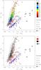 |
Fig. 2 V−I vs. J−K colour–colour diagram of C1 (circles) and C3 (triangles) subsamples. The colours indicate the spectral type (upper panel) and luminosity class (lower panel). The photometric calibrations of Worthey & Lee (2011) are depicted by three dashed-dotted lines corresponding to iso-gravity contours, from left to right, of log g = 3, 2 and 0 dex. The small black dots indicate the location of hydrostatic carbon stars from the models by Aringer et al. (2009). The stars previously classified as carbon stars are depicted by a square symbol. The stars from the samples towards the outer regions of the Galaxy are indicated by open red circles, while the stars from the LRc03 CoRoT Run are identified using blue open circles. The error bars in the bottom right corner of the two diagrams represent the typical uncertainties for the colours (ϵ(V−I) = 0.29 mag and ϵ(J−K) = 0.09 mag). |
The C1 and C3 sources are used to describe the evolutionary and variability behaviour of M giant-type stars in forward sections.
3. Results
We report our results in the following sections, using a final sample of 1314 M-giants (C1 and C3 stars). First, we perform an analysis of the V−I versus J−K colour diagram and compare our results to the models of Aringer et al. (2009) and the empirical calibrations of Worthey & Lee (2011) and to other works from the literature. Then we discuss and interpret our results using the period-amplitude and the period-Teff diagrams. Afterwards, we compare the results of the measured period and amplitude from the stars located towards the inner and outer regions of the Galaxy. Finally, we discuss the lack of short-time variations in M giants, and make a brief mention of the Mira-variable stars and the carbon stars that we have in common with other works.
3.1. The evolutionary behaviour along the colour–colour diagram
Figure 2 shows the colour–colour diagrams of our C1 (full circles) and C3 (Teff< 4200 K – 105 stars) (full triangles) subsamples, where the colours set the spectral type (upper panel) and luminosity class (lower panel). Here we only consider stars with V-, I-, J-, and KS-band photometry. We note that the reddening may not only be caused by interstellar, but also by circumstellar reddening (Lebzelter 2011)
The corrected colours show a reasonable agreement with the empirical calibrations of Worthey & Lee (2011). However, there are two groups of stars that do not follow this trend. One group, with a lower average value of V−I situated between the photometric calibrations and the synthetic photometry from hydrostatic models of C-rich giants from Aringer et al. (2009). Nevertheless, only an abundance analysis would enable us to determine whether these targets are carbon stars. Interestingly, almost all stars from this subgroup belong to the CoRoT anticentre fields. We do not know the reason for this behaviour, but we hypothesise that the samples towards the inner and outer regions of the Galaxy may belong to two different galactic populations. In fact, an increasing trend of the C star/M star ratio with [Fe/H] in the Galaxy is reported in the literature (e.g., Frebel et al. 2006) and in the Large Magellanic Cloud (Blanco et al. 1980; Cioni & Habing 2003). At the same time, a negative trend with [Fe/H] has been reported by a variety of studies (e.g., Boeche et al. 2013; Bergemann et al. 2014), at low values of galactic vertical height (| Z | < 300−400 pc). Therefore, a possible explanation for the imbalance of C stars between the two fields may be related to the negative [Fe/H] trend as a function of the galactic radius. Our results are in close agreement with those presented in Fig. 2 of Lebzelter (2011).
We also observe that most of the supergiant population (Type I) has a lower value of V−I for the same J−K colour when compared to the two groups of giant stars and are located below the predicted region for C-rich stars. For J−K> 1.3, the location of these stars coincide with the models, but theoretical traces from Aringer et al. (2009) do not cover spectral Class I. We note that the large majority of the stars from this group belong to the LRc03 field towards the inner regions of the Galaxy.
The LPVs Candidates (C3 catalogue) are distributed throughout the colour–colour diagram. This is to be expected since the time span of the LPVs range from 24 to 145 days, implying a greater variability period. Eight of 12 stars with V−I> 3.8 have a total time span greater than 100 days (and therefore a greater period). These aspects agree with the period versus Teff trend (Fig. 3, lower panels), since we expect long periods for stars with lower temperatures (and higher V−I colour). This result strongly suggests that long-term trends found for all candidates of LPVs may be real.
3.2. The period variability and amplitude behaviour
To investigate the nature of the stellar photometric variability identified in the present work, we studied the period variability as a function of amplitude and effective temperature for stars of the present sample that exhibit semi–sinusoidal behaviour in their observed LCs. We have therefore used the periods and amplitudes for the sample of 1173 stars described in Sect. 2.4 (the C1 catalogue). To study the multi-mode behaviour, we considered the first three independent frequencies on the period-amplitude diagrams of Fig. 3. In the case of the Teff-period diagrams, we only used the main period.
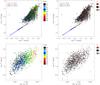 |
Fig. 3 Distribution of variability period as a function of the amplitude and the effective temperature for C1 stars. The colours indicate the spectral type (left panels) and luminosity class (right panels). The large circles in the upper panels mark the main variability period and the small circles mark the secondary periods. In the lower panels, only the main variability period is shown. The red line between the two red crosses roughly depict the trend of the overtone (AB) pulsators taken from Fig. 15 of Tabur et al. (2010). The blue line between the two blue crosses represents the area defined by Bányai et al. (2013), selected from the top panel of Fig. 3 of Huber et al. (2011), where solar-like oscillations are expected to be found. The two black lines indicate the two distinct Amplitude-νmax relations for solar-type oscillators found by Mosser et al. (2013, their Eqs. (8) and (9)). |
The distribution of the multi-modes as a function of the amplitude is displayed in Fig. 3 (upper panels). The circles represent the stronger mode, while the dots depict the other modes of oscillation. The red line between the two red crosses roughly depicts the trend of the overtone (AB) pulsators taken from Fig. 15 of Tabur et al. (2010). The blue line between the two blue crosses represents the area defined by Bányai et al. (2013), selected from the top panel of Fig. 3 of Huber et al. (2011), where solar-like oscillations are expected to be found. The two black lines indicate the two distinct amplitude-νmax relations for solar-type oscillators found by Mosser et al. (2013, their Eqs. (8) and (9)).
The observed period-amplitude behaviour clearly parallels the classic scenario for the pulsation period-amplitude relation that has been well established for M-giant stars with semi-sinusoidal variations using different stellar samples observed from the ground (e.g., Alard et al. 2001; Wray et al. 2004; Tabur et al. 2010).
The scenario presented in Fig. 3 (upper panels) for the stronger pulsation (open circles) follows the trend observed by Tabur et al. (2010) closely (red line in the diagram), which corresponds to stars pulsating in overtones. The other modes of oscillation agree well with the amplitude-νmax relation of Mosser et al. (2013) for ν< 1 μHz, corresponding to log P> 1.06 days. The two distinct relations suggest that there are two different oscillation mechanisms: the stronger one, characteristic of self-excited Mira-like pulsations; the smaller amplitude ones, mimicking the behaviour of solar-type oscillations.
Our finding also agrees with the results of Bányai et al. (2013), who, on the basis of Kepler observations of M-type giant stars (their group 3), found a similar period-amplitude behaviour. Group 3, as defined by those authors, contains stars with LCs that exhibit only a few periodic components (like Miras and SRs) that agree with the signatures of semi-sinusoidal variables. Bányai et al. (2013) also reported a sharp break at log P~ 1 day (corresponding to 1.2 μHz), marking the end of the clear correlation between their Group 2 and their adapted relation from amplitude-νmax relation of Huber et al. (2011). We do not observe a trend in our Fig. 3 (upper panels) in the same region of log P. However, we must note we have very few periods with similar amplitudes in that period region. Despite this, if we only account for the stronger pulsation, we observe, by eye, that there is a slight change in the slope around log P ~ 1 day.
We also analysed the relation period Teff. Figure 3 (lower panels) shows all 1141 giant stars from our C1 sample with semi-sinusoidal variations, where only the primary computed pulsation period is considered. We observe a correlation of the period of the main oscillation with Teff similar to the trend found by Huber et al. (2011) for hotter giants from the Kepler sample, with the oscillation frequency vmax. A careful comparison of our Fig. 3 (bottom left panel) with Fig. 8 of Huber et al. (2011), suggests an agreement between both trends. Indeed, the feature revealed from Fig. 3 (lower panels) seems to correspond to an extension of the upper part of the modified H–R diagram (Fig. 8) of Huber et al. (2011).
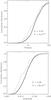 |
Fig. 4 Cumulative distribution function of the period (left panel) and amplitude (right panel) for stars in the inner (solid line) and outer (dashed line) regions of the Galaxy. |
3.3. The inner and outer regions of the Galaxy
To verify whether the behaviour of the variability of sources from the inner and outer regions of the Galaxy are significantly different, we applied the Kuiper test (or invariant KS test – hereafter the KS test) (e.g., Jetsu & Pelt 1996; Paltani 2004) to our C1 subgroup. The C1 is composed of 1124 stars located towards inner regions of the Galaxy, and 91 in the outer regions. According to the KS test, zero probability means that the distributions are dissimilar, whereas unit probability means they are drawn from the same parent distribution.
Figure 4 shows the cumulative distribution function of the amplitude and period of C1 stars. The solid black distribution depicts the stars located in the inner regions, whereas the dashed grey distribution describes the outer region. The obtained p values for the amplitude and period distributions are lower than 10-3. This result shows that there is a very low probability that the two samples belong to the same parent distribution. The difference between the two samples may also be observed in the colour–colour diagram (Fig. 2), where most stars from the outer region sample are in the region commonly associated with carbon stars, while the sample from the inner region of the Galaxy are mostly M giants. Also, the metallicity of our two samples should be different (see Sect. 3.1), and this may play an important role in M Giant evolution, since these distributions are dissimilar in terms of amplitude and period.
We tested the KS test by perturbing our two samples. First, we withdrew a random quantity of stars from our sample (between 5% to 10%) using a uniform Monte Carlo distribution and next, we performed the KS test. This process was iterated 1000 times. The higher 3σ value taken from the median of the amplitude and period distribution was 0.002 and 0.05, respectively. The indicative of dissimilarity is not robust enough for the period distribution.
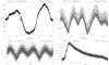 |
Fig. 5 CoRoT 652190748 and CoRoT 104849311 light curves (upper panels). The red line indicates a boxcar smoothed version of the LC. The phase diagrams of their short-time variations are depicted in the lower panels. The CoRoT-ID and period are presented in each panel. |
3.4. Short-time variations of CoRoT M-giant stars
The CoRoT data have at least a 512-s sampling interval and a long coverage period that allow us to study the occurrence of rapid outbursts or very short-time variations in LPVs on very short timescales (from hours to a few days). These variation changes of several tenths of magnitudes should occur once per star per year according to the literature (Woźniak et al. 2004). A recent study, using a sample of 52 CoRoT stars (Lebzelter 2011) and 9 Kepler stars (Hartig et al. 2014), presented no detections of such rapid variations for amplitudes above 0.01 mag. However, only a small number of sources were analysed.
A detailed search by visual inspection on the LCs of all CoRoT M-giant stars making up the present sample did not yield any short-term event. All outburst-like variations that were found may be related to hot pixel events or other instrumental artefacts (check, for instance, the LC panels of CoRoT 105731070, 105832319, and 105965810 of Fig. 1). This agrees with other recent studies, showing that this phenomenon is rare or does not exist (e.g., Woźniak et al. 2004; Lebzelter 2011; Hartig et al. 2014). Taking all results from different instruments and small and large samples into account, we can conclude that the short-time outbursts (<1 day) in long-period variables do not exist or, at least, are very rare events.
Another possible cause of a false outburst event may lie with a background star. In this case, the observed variation will be the superposition of the signal from both stars. Figure 5 shows two CoRoT LPVs where the phase diagrams (lower panels) show a signature of a background binary (left panel) and a RR-Lyrae (right panel) star. To study the short-time variation in the two LCs, a pre-whitened curve was obtained by dividing each LC by a boxcar smoothing function of the curve itself. Then, the period was computed using a similar proceedure, as described in Sect. 2.3.
3.5. Long-period variables
Three LPVs stars of our sample were previously analysed by Lebzelter (2011) using CoRoT data. Some of these stars are also common to the AAVSO International Variable Star Index (Watson et al. 2014) catalogue. In the present LPVs sample (C3) we identify four Mira variable stars, CoRoT 104982243, 105580931, 632685506, and 653546843, with previously computed periods of 329, 205, 195, and 116 days, respectively (Watson et al. 2014).
3.6. Carbon-type stars
Eight carbon-type stars, previously described in the literature (MacConnell 1988; Stephenson 1989, 1996; Alksnis et al. 2001; Chen & Yang 2012; Zacharias et al. 2013; Watson et al. 2014), are identified in our sample. These stars are in the fields towards the outer regions of the Galaxy (LRa01, IRa01, and LRa02 CoRoT runs). The combination of different CoRoT runs allows us to study the long periods of the carbon stars with more accuracy. For instance, CoRoT-ID 102760221 (see Fig. 1 last row, right panel) was analysed by Lebzelter (2011) using the CoRoT Runs IRa01 and LRa01. A period of 116 days is reported by Lebzelter (2011) as the probable main period, once its LC present a minimum and a maximum between 250 and 400 days. Because the CoRoT-ID 102760221 was re-observed during the LRa06 Run, we have combined all the observations (CoRoT Runs IRa01, LRa01, and LRa06) for a check of the period measurements, finding now a period of 349 days that may be related with the fundamental pulsation mode.
On the other hand, in some cases, the total time span is not long enough to provide a reliable period (see Fig. 6, upper panel), while in other cases, we can observe more than one cycle (Fig. 6, lower panel). For instance, the star CoRoT 110663214 displays a period of 68 days. However, the shape of its LC indicates the existence of a larger period. Using the methodology of De Medeiros et al. (2013), we obtain a confidence level of about 70% for this period.
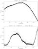 |
Fig. 6 LCs of two previously identified carbon type stars: CoRoT 110838652 and 110663214. |
4. Conclusions
In this work we have performed a study of the semi-sinusoidal variability behaviour of CoRoT M giant stars. This is the largest detailed study of M giants observed by CoRoT, and it provides an opportunity for comparison with previous works based on space missions like CoRoT and Kepler (e.g., Lebzelter 2011; Bányai et al. 2013; Huber et al. 2014; Hartig et al. 2014) and on ground-based observations (e.g., Alard et al. 2001; Wray et al. 2004; Tabur et al. 2010).
We also present a CoRoT variability list for M-giant stars. The C1 sample, which contains 1173 objects, is composed of all stars classified as M giants in the CoRoT database with Teff< 4200 K. These were identified via visual inspection as semi-sinusoidal variables. The effective temperature Teff was estimated from the calibration of van Belle et al. (1999) using V−K colour indices. The main variability period spans from ~2 to ~152 days, with the amplitude ranging from ~1 to ~900 mmag. The C2 sample is comprised of 141 stars that exhibit semi-sinusoidal variations (with Teff> 4200 K), and the C3 sample contains 114 LPV candidates. The last two subsamples may be considered for follow-up observations to study their variability nature.
We cross-checked our data with previously published catalogues and found 444 targets in common. The computed periods are similar (i.e., discrepancy less than 10%) for 96% of these targets, which indicates good agreement between our results and previous results from the literature. The cross-matched sources were used to withdraw misclassification and to identify comparison stars.
The location of the majority of the sample stars in the V−I versus J−K colour–colour diagram shows good agreement with the empirical calibrations of Worthey & Lee (2011). Two groups of stars present different trends. The first one, with a lower average value of V−I for the same J−K is mostly composed of stars from the outer region sample, and is located between the Giant calibrations and the carbon-star models of Aringer et al. (2009). The second group, located in the lowest V−I region of the diagram, appears to be mostly composed of a Type I supergiant population. The large majority of the stars from this group belong to the LRc03 field towards the inner regions of the Galaxy.
We considered the first three periods with significance levels greater than 99% to study their behaviour in a period-amplitude diagram. The distribution exhibits a trend towards increasing amplitude with increasing period, which is compatible with the expected behaviour for stellar pulsation (e.g., Alard et al. 2001; Wray et al. 2004; Tabur et al. 2010). We also observe that the main variability period follows closely the stars identified by Tabur et al. (2010) as overtone pulsators. The less powerful periods follow the trend formulated by Mosser et al. (2013) for solar-like oscillations. A similar analysis was performed using a period versus Teff diagram, which exhibits a trend towards increasing period with decreasing temperature. This trend is compatible with a previous study based on Kepler observations for GK giants (Huber et al. 2011), and our new data confirms that the behaviour of the period–effective temperature relation extends to the cooler M-giant stars.
Regarding the short-time variations on M-giant stars previously reported in the literature, we also concluded that they do not exist or are very rare. The few cases we found are related to biases or background stars.
Acknowledgments
We would like to thank Evelin Banyai for useful discussions. The authors would also like to thank the anonymous referee for valuable comments and suggestions that greatly improved this paper. Research activities of the Observational Stellar Board of the Federal University of Rio Grande do Norte are supported by the continuous grants of the CNPq and FAPERN Brazilian agencies and by the INCT-INEspaço. C.E.F.L. acknowledges a post-doctoral fellowships from the CNPq. C.E.F.L. also thanks the Royal Observatory Edinburgh for hospitality. V.N. acknowledges a CNPq/BJT post-doctoral fellowship 301186/2014-6. I.C.L. acknowledges post-doctoral PNPD/CNPq and post-doctoral PDE/CNPq fellowships. I.C.L. also thanks ESO/Garching for hospitality. M.L.C. acknowledges post-doctorate fellowship of the CAPES brazilian agency. F.P.Ch. and A.D.C. acknowledge PhD fellowships from the CNPq. This research made use of the NASA/IPAC Infrared Science Archive, which is operated by the Jet Propulsion Laboratory, California Institute of Technology, under contract with the National Aeronautics and Space Administration (NASA).
References
- Affer, L., Micela, G., Favata, F., & Flaccomio, E. 2012, MNRAS, 424, 11 [NASA ADS] [CrossRef] [Google Scholar]
- Alard, C., Blommaert, J. A. D. L., Cesarsky, C., et al. 2001, ApJ, 552, 289 [NASA ADS] [CrossRef] [Google Scholar]
- Alksnis, A., Balklavs, A., Dzervitis, U., et al. 2001, Baltic Astron., 10, 1 [Google Scholar]
- Aringer, B., Girardi, L., Nowotny, W., Marigo, P., & Lederer, M. T. 2009, A&A, 503, 913 [NASA ADS] [CrossRef] [EDP Sciences] [Google Scholar]
- Auvergne, M., Bodin, P., Boisnard, L., et al. 2009, A&A, 506, 411 [NASA ADS] [CrossRef] [EDP Sciences] [Google Scholar]
- Baglin, A., Auvergne, M., Barge, P., et al. 2007, in Fifty Years of Romanian Astrophysics, eds. C. Dumitrache, N. A. Popescu, M. D. Suran, & V. Mioc, AIP Conf. Ser., 895, 201 [Google Scholar]
- Bányai, E., Kiss, L. L., Bedding, T. R., et al. 2013, MNRAS, 436, 1576 [NASA ADS] [CrossRef] [Google Scholar]
- Basri, G., Walkowicz, L. M., Batalha, N., et al. 2011, AJ, 141, 20 [NASA ADS] [CrossRef] [Google Scholar]
- Batalha, N. M., Rowe, J. F., Bryson, S. T., et al. 2013, ApJS, 204, 24 [NASA ADS] [CrossRef] [Google Scholar]
- Bedding, T. R., Kiss, L. L., Kjeldsen, H., et al. 2005, MNRAS, 361, 1375 [NASA ADS] [CrossRef] [Google Scholar]
- Bergemann, M., Kudritzki, R.-P., & Davies, B. 2014, ArXiv e-prints [arXiv:1403.3087] [Google Scholar]
- Blanco, V. M., Blanco, B. M., & McCarthy, M. F. 1980, ApJ, 242, 938 [NASA ADS] [CrossRef] [Google Scholar]
- Boeche, C., Chiappini, C., Minchev, I., et al. 2013, A&A, 553, A19 [NASA ADS] [CrossRef] [EDP Sciences] [Google Scholar]
- Borucki, W. J., Koch, D., Basri, G., et al. 2010, Science, 327, 977 [NASA ADS] [CrossRef] [PubMed] [Google Scholar]
- Borucki, W. J., Koch, D. G., Batalha, N., et al. 2012, ApJ, 745, 120 [NASA ADS] [CrossRef] [Google Scholar]
- Brown, T. M., Latham, D. W., Everett, M. E., & Esquerdo, G. A. 2011, AJ, 142, 112 [NASA ADS] [CrossRef] [Google Scholar]
- Carpenter, J. M. 2001, AJ, 121, 2851 [NASA ADS] [CrossRef] [Google Scholar]
- Chen, P. S., & Yang, X. H. 2012, AJ, 144, 104 [NASA ADS] [CrossRef] [Google Scholar]
- Christensen-Dalsgaard, J., Kjeldsen, H., & Mattei, J. A. 2001, ApJ, 562, L141 [NASA ADS] [CrossRef] [Google Scholar]
- Cioni, M.-R. L., & Habing, H. J. 2003, A&A, 402, 133 [NASA ADS] [CrossRef] [EDP Sciences] [Google Scholar]
- de Freitas, D. B., Leão, I. C., Ferreira Lopes, C. E., et al. 2013, ApJ, 773, L18 [NASA ADS] [CrossRef] [Google Scholar]
- de Laverny, P., Mennessier, M. O., Mignard, F., & Mattei, J. A. 1998, A&A, 330, 169 [NASA ADS] [Google Scholar]
- Deleuil, M., Meunier, J. C., Moutou, C., et al. 2009, AJ, 138, 649 [NASA ADS] [CrossRef] [Google Scholar]
- De Medeiros, J. R., Ferreira Lopes, C. E., Leão, I. C., et al. 2013, A&A, 555, A63 [NASA ADS] [CrossRef] [EDP Sciences] [Google Scholar]
- Dressing, C. D., & Charbonneau, D. 2013, ApJ, 767, 95 [NASA ADS] [CrossRef] [Google Scholar]
- Dworetsky, M. M. 1983, MNRAS, 203, 917 [NASA ADS] [Google Scholar]
- Dziembowski, W. A., & Soszyński, I. 2010, A&A, 524, A88 [NASA ADS] [CrossRef] [EDP Sciences] [Google Scholar]
- Dziembowski, W. A., Gough, D. O., Houdek, G., & Sienkiewicz, R. 2001, MNRAS, 328, 601 [NASA ADS] [CrossRef] [Google Scholar]
- Eaton, N. L., Herbst, W., & Hillenbrand, L. A. 1995, AJ, 110, 1735 [NASA ADS] [CrossRef] [Google Scholar]
- Frebel, A., Christlieb, N., Norris, J. E., et al. 2006, ApJ, 652, 1585 [NASA ADS] [CrossRef] [Google Scholar]
- Guenther, E. W., Gandolfi, D., Sebastian, D., et al. 2012, A&A, 543, A125 [NASA ADS] [CrossRef] [EDP Sciences] [Google Scholar]
- Hartig, E., Cash, J., Hinkle, K. H., et al. 2014, AJ, 148, 123 [NASA ADS] [CrossRef] [Google Scholar]
- Hekker, S., Elsworth, Y., Mosser, B., et al. 2013, A&A, 556, A59 [NASA ADS] [CrossRef] [EDP Sciences] [Google Scholar]
- Hoffman, D. I., Harrison, T. E., & McNamara, B. J. 2009, AJ, 138, 466 [NASA ADS] [CrossRef] [Google Scholar]
- Huber, D., Bedding, T. R., Stello, D., et al. 2011, ApJ, 743, 143 [NASA ADS] [CrossRef] [Google Scholar]
- Huber, D., Ireland, M. J., Bedding, T. R., et al. 2012, ApJ, 760, 32 [NASA ADS] [CrossRef] [Google Scholar]
- Huber, D., Silva Aguirre, V., Matthews, J. M., et al. 2014, ApJS, 211, 2 [NASA ADS] [CrossRef] [Google Scholar]
- Jetsu, L., & Pelt, J. 1996, A&AS, 118, 587 [NASA ADS] [CrossRef] [EDP Sciences] [Google Scholar]
- Kazarovets, E. V., Samus, N. N., & Durlevich, O. V. 1998, IBVS, 4655, 1 [NASA ADS] [Google Scholar]
- Kiss, L. L., & Bedding, T. R. 2003, MNRAS, 343, L79 [NASA ADS] [CrossRef] [Google Scholar]
- Lanza, A. F., Das Chagas, M. L., & De Medeiros, J. R. 2014, A&A, 564, A50 [NASA ADS] [CrossRef] [EDP Sciences] [Google Scholar]
- Lebzelter, T. 2011, A&A, 530, A35 [NASA ADS] [CrossRef] [EDP Sciences] [Google Scholar]
- Lebzelter, T., Schultheis, M., & Melchior, A. L. 2002, A&A, 393, 573 [NASA ADS] [CrossRef] [EDP Sciences] [Google Scholar]
- Léger, A., Rouan, D., Schneider, J., et al. 2009, A&A, 506, 287 [NASA ADS] [CrossRef] [EDP Sciences] [MathSciNet] [Google Scholar]
- Lomb, N. R. 1976, Ap&SS, 39, 447 [NASA ADS] [CrossRef] [Google Scholar]
- MacConnell, D. J. 1988, AJ, 96, 354 [NASA ADS] [CrossRef] [Google Scholar]
- Maceroni, C., Montalbán, J., Michel, E., et al. 2009, A&A, 508, 1375 [NASA ADS] [CrossRef] [EDP Sciences] [Google Scholar]
- Maciel, S. C., Osorio, Y. F. M., & De Medeiros, J. R. 2011, New A, 16, 68 [Google Scholar]
- Maffei, P., & Tosti, G. 1995, AJ, 109, 2652 [NASA ADS] [CrossRef] [Google Scholar]
- Mais, D. E., Stencel, R. E., & Richards, D. 2004, J. Am. Assoc. Variable Star Observers (JAAVSO), 33, 48 [NASA ADS] [Google Scholar]
- McQuillan, A., Aigrain, S., & Mazeh, T. 2013, MNRAS, 432, 1203 [NASA ADS] [CrossRef] [MathSciNet] [Google Scholar]
- Morton, T. D., & Swift, J. 2014, ApJ, 791, 10 [NASA ADS] [CrossRef] [Google Scholar]
- Mosser, B., Belkacem, K., Goupil, M.-J., et al. 2010, A&A, 517, A22 [NASA ADS] [CrossRef] [EDP Sciences] [Google Scholar]
- Mosser, B., Dziembowski, W. A., Belkacem, K., et al. 2013, A&A, 559, A137 [NASA ADS] [CrossRef] [EDP Sciences] [Google Scholar]
- Nielsen, M. B., Gizon, L., Schunker, H., & Karoff, C. 2013, A&A, 557, L10 [NASA ADS] [CrossRef] [EDP Sciences] [Google Scholar]
- Paltani, S. 2004, A&A, 420, 789 [NASA ADS] [CrossRef] [EDP Sciences] [Google Scholar]
- Renner, S., Rauer, H., Erikson, A., et al. 2008, A&A, 492, 617 [NASA ADS] [CrossRef] [EDP Sciences] [Google Scholar]
- Riebel, D., Meixner, M., Fraser, O., et al. 2010, ApJ, 723, 1195 [NASA ADS] [CrossRef] [Google Scholar]
- Samus, N. N., Durlevich, O. V., et al. 2009, VizieR Online Data Catalog B/gcvs [Google Scholar]
- Sarro, L. M., Debosscher, J., Neiner, C., et al. 2013, A&A, 550, A120 [NASA ADS] [CrossRef] [EDP Sciences] [Google Scholar]
- Scargle, J. D. 1982, ApJ, 263, 835 [NASA ADS] [CrossRef] [Google Scholar]
- Schaefer, B. E. 1991, ApJ, 366, L39 [NASA ADS] [CrossRef] [Google Scholar]
- Schlafly, E. F., & Finkbeiner, D. P. 2011, ApJ, 737, 103 [NASA ADS] [CrossRef] [Google Scholar]
- Schlafly, E. F., Green, G., Finkbeiner, D. P., et al. 2014, ApJ, 789, 15 [NASA ADS] [CrossRef] [Google Scholar]
- Sebastian, D., Guenther, E. W., Schaffenroth, V., et al. 2012, A&A, 541, A34 [NASA ADS] [CrossRef] [EDP Sciences] [Google Scholar]
- Silva Aguirre, V., Casagrande, L., Basu, S., et al. 2012, ApJ, 757, 99 [NASA ADS] [CrossRef] [Google Scholar]
- Skrutskie, M. F., Cutri, R. M., Stiening, R., et al. 2006, AJ, 131, 1163 [NASA ADS] [CrossRef] [Google Scholar]
- Slawson, R. W., Prša, A., Welsh, W. F., et al. 2011, AJ, 142, 160 [NASA ADS] [CrossRef] [Google Scholar]
- Soszynski, I., Dziembowski, W. A., Udalski, A., et al. 2007, Acta Astron., 57, 201 [NASA ADS] [Google Scholar]
- Soszyński, I., Wood, P. R., & Udalski, A. 2013, ApJ, 779, 167 [NASA ADS] [CrossRef] [Google Scholar]
- Stello, D., Compton, D. L., Bedding, T. R., et al. 2014, ApJ, 788, L10 [NASA ADS] [CrossRef] [Google Scholar]
- Stephenson, C. B. 1989, Publications of the Warner & Swasey Observatory, 3, 53 [Google Scholar]
- Stephenson, C. B. 1996, VizieR Online Data Catalog: III/156 [Google Scholar]
- Tabur, V., Bedding, T. R., Kiss, L. L., et al. 2010, MNRAS, 409, 777 [NASA ADS] [CrossRef] [Google Scholar]
- Taylor, M. B. 2005, in Astronomical Data Analysis Software and Systems XIV, eds. P. Shopbell, M. Britton, & R. Ebert, ASP Conf. Ser., 347, 29 [Google Scholar]
- van Belle, G. T., Lane, B. F., Thompson, R. R., et al. 1999, AJ, 117, 521 [NASA ADS] [CrossRef] [Google Scholar]
- Walkowicz, L. M., & Basri, G. S. 2013, MNRAS, 436, 1883 [NASA ADS] [CrossRef] [Google Scholar]
- Watson, C., Henden, A. A., & Price, A. 2014, VizieR Online Data Catalog B/vsx [Google Scholar]
- Wiśniewski, M., Marquette, J. B., Beaulieu, J. P., et al. 2011, A&A, 530, A8 [NASA ADS] [CrossRef] [EDP Sciences] [Google Scholar]
- Wood, P. R., & Sebo, K. M. 1996, MNRAS, 282, 958 [NASA ADS] [CrossRef] [Google Scholar]
- Worthey, G., & Lee, H.-C. 2011, ApJS, 193, 1 [NASA ADS] [CrossRef] [EDP Sciences] [Google Scholar]
- Woźniak, P. R., McGowan, K. E., & Vestrand, W. T. 2004, ApJ, 610, 1038 [NASA ADS] [CrossRef] [Google Scholar]
- Wray, J. J., Eyer, L., & Paczyński, B. 2004, MNRAS, 349, 1059 [NASA ADS] [CrossRef] [Google Scholar]
- Zacharias, N., Finch, C. T., Girard, T. M., et al. 2013, AJ, 145, 44 [NASA ADS] [CrossRef] [EDP Sciences] [Google Scholar]
All Tables
CoRoT M-type stars taken from EXO-Dat (Deleuil et al. 2009) distributed by luminosity class.
All Figures
|
Fig. 1 Typical LCs of stars from our catalogue. CoRoT-ID and period of the C1 (row 1–3) and C2 (row 4) catalogues are shown in the headers. For the C3 (LPVs – row 5) sources, only the CoRoT-ID is shown. The red line indicates the harmonic fit models of the C1 stars given by Eq. (2). |
| In the text | |
|
Fig. 2 V−I vs. J−K colour–colour diagram of C1 (circles) and C3 (triangles) subsamples. The colours indicate the spectral type (upper panel) and luminosity class (lower panel). The photometric calibrations of Worthey & Lee (2011) are depicted by three dashed-dotted lines corresponding to iso-gravity contours, from left to right, of log g = 3, 2 and 0 dex. The small black dots indicate the location of hydrostatic carbon stars from the models by Aringer et al. (2009). The stars previously classified as carbon stars are depicted by a square symbol. The stars from the samples towards the outer regions of the Galaxy are indicated by open red circles, while the stars from the LRc03 CoRoT Run are identified using blue open circles. The error bars in the bottom right corner of the two diagrams represent the typical uncertainties for the colours (ϵ(V−I) = 0.29 mag and ϵ(J−K) = 0.09 mag). |
| In the text | |
|
Fig. 3 Distribution of variability period as a function of the amplitude and the effective temperature for C1 stars. The colours indicate the spectral type (left panels) and luminosity class (right panels). The large circles in the upper panels mark the main variability period and the small circles mark the secondary periods. In the lower panels, only the main variability period is shown. The red line between the two red crosses roughly depict the trend of the overtone (AB) pulsators taken from Fig. 15 of Tabur et al. (2010). The blue line between the two blue crosses represents the area defined by Bányai et al. (2013), selected from the top panel of Fig. 3 of Huber et al. (2011), where solar-like oscillations are expected to be found. The two black lines indicate the two distinct Amplitude-νmax relations for solar-type oscillators found by Mosser et al. (2013, their Eqs. (8) and (9)). |
| In the text | |
|
Fig. 4 Cumulative distribution function of the period (left panel) and amplitude (right panel) for stars in the inner (solid line) and outer (dashed line) regions of the Galaxy. |
| In the text | |
|
Fig. 5 CoRoT 652190748 and CoRoT 104849311 light curves (upper panels). The red line indicates a boxcar smoothed version of the LC. The phase diagrams of their short-time variations are depicted in the lower panels. The CoRoT-ID and period are presented in each panel. |
| In the text | |
|
Fig. 6 LCs of two previously identified carbon type stars: CoRoT 110838652 and 110663214. |
| In the text | |
Current usage metrics show cumulative count of Article Views (full-text article views including HTML views, PDF and ePub downloads, according to the available data) and Abstracts Views on Vision4Press platform.
Data correspond to usage on the plateform after 2015. The current usage metrics is available 48-96 hours after online publication and is updated daily on week days.
Initial download of the metrics may take a while.