© ESO, 2015

1. Introduction

The X-ray source XB 1916-053 is a low-mass X-ray binary (LMXB) showing dips and type-I X-ray bursts in its light curves. Using OSO 8 data, Becker et al. (1977) observed type-I X-ray bursts, implying that the compact source in XB 1916-053 is a neutron star. Assuming that the peak luminosity of the X-ray bursts in XB 1916-053 is at the Eddington limit, Smale et al. (1988) derived a distance to the source of 8.4 kpc or 10.8 kpc, respectively, depending on whether the accreting matter has cosmic abundances or is extremely hydrogen-deficient. Yoshida (1993) inferred a distance to the source of 9.3 kpc studying the photospheric radius expansion of the X-ray bursts in XB 1916-053 (see also Barret et al. 1996). XB 1916-053 was the first LMXB in which periodic absorption dips were detected (Walter et al. 1982; White & Swank 1982). These dips represent a decrease in the count rate in the light curve caused by periodic absorption of the X-ray emission produced in the inner region of the system. The photoelectric absorption occurs in a bulge at the outer radius of the accretion disc where the matter streaming from a companion star impacts.

Accurate analysis of data sets from many X-ray satellites in the last 30 years have found different values for the X-ray period: Walter et al. (1982) found a period close to 2985 s, using Einstein data; White & Swank (1982) estimated a period of 3003.6 ± 1.8 s for the strongest dips, while Smale et al. (1989), analysing Ginga data, derived a period of 3005.0 ± 6.6 s. Church et al. (1997), analysing ASCA data, found an orbital period of 3005 ± 10 s. The X-ray light curve of XB 1916-053 also shows secondary dips occurring approximately half a cycle away from the primary dips with a certain variability in phase (see Grindlay 1989). No eclipses were found; this constrains the orbital inclination of the system between 60° and 80°.

The optical counterpart of XB1916-053 was discovered by Grindlay et al. (1987), a star with a V magnitude of 21 already noted by Walter et al. (1982). Using thermonuclear flash models of X-ray bursts, Swank et al. (1984) argued that the companion star is not hydrogen exhausted and suggested a companion star mass of 0.1 M_⊙. Furthermore, Paczynski & Sienkiewicz (1981) showed that X-ray binary systems with orbital periods shorter than 81 min cannot contain hydrogen-rich secondary stars.

A modulation in the optical light curve with a period of 3027.4 ± 0.4 s was discovered by Grindlay et al. (1988). The 1% discrepancy between the optical and X-ray period of XB 1916-053 was explained by Grindlay et al. (1988) invoking the presence of a third body with a period of 2.5 d and a retrograde orbit that influences the matter streaming from the companion star. The same authors also suggested the alternative scenario in which the disc bulge precesses around the disc with a prograde period equivalent to the beat period between the optical and X-ray period. White (1989) suggested the possibility that a precessing elliptical disc exists in XB 1916-053, and that the variation in the projected area of this disc causes optical modulation. Callanan et al. (1995) showed the stability of the optical period over seven years. Chou et al. (2001), analysing Rossi X-ray Timing Explorer (RXTE) data taken in 1996, found several periodicities including one at 3026.23 ± 3.23 s, which was similar to the optical modulation at 3027 s. The centroid of these peaks in the periodogram associated with the 3000 s period implies that there is a modulation with a fundamental period close to 3.9 d, as already noticed by Grindlay (1992) also in the optical band. The period of 3.9 d is interpreted as the beat period between the optical and X-ray periods. Furthermore, Chou et al. (2001), folding the RXTE light curves at the 3.9 d period, found changes in the dip shape following this modulation. Those authors also indicated that the dip-phase change, with a sinusoidal period of 6.5 ± 1.1 d from Ginga 1990 September observations (Yoshida 1993; Yoshida et al. 1995), may be associated with the subharmonic of the 3.9 d period. Retter et al. (2002) detected a further independent X-ray period at 2979 s in the RXTE light curves of XB 1916-053, which was mistakenly identified by Chou et al. (2001) with a 3.9 d sideband of the 3000 s period. Retter et al. (2002) suggested that the period at 2979 s could be explained as a negative super-hump assuming the 3000 s period is the orbital period with a corresponding beat period of 4.8 d. The same authors suggested that the 3.9 and 4.8 d periods could be the apsidal and nodal precession of the accretion disc, respectively.

Finally, the source also showed a long-term 198.6 ± 1.72 d periodicity in X-rays (Priedhorsky & Terrell 1984), which has not been confirmed by further observations (see Retter et al. 2002). To date the spin period of the neutron star in XB 1916-053 is not known. Galloway et al. (2001), analysing a Type-I X-ray burst, discovered a highly coherent oscillation drifting from 269.4 Hz up to 272 Hz. Interpreting the asymptotic frequency of the oscillation in terms of a decoupled surface burning layer, the neutron star could have a spin period around 3.7 ms.

Hu et al. (2008) inferred that Ṗ_orb/P_orb = (1.62 ± 0.34) × 10^-7 yr^-1 by analysing archival X-ray data from 1978 to 2002 and adopting a quadratic ephemeris to fit the dip arrival times. In this work, we update the previously determined ephemeris using data from 1978 to 2014. We show that the quadratic ephemeris does not fit the dip arrival times and find that a sinusoidal component is necessary to fit the delays. We suggest the presence of a third body that influences the orbit of the X-ray binary system XB 1916-053.

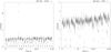Fig. 1 Chandra/LEG light curves of XB 1916-053 during the two observations performed in 2013, i.e. obsid. 15271 (left) and 15657 (right). The bin time is 64 s. A type-I X-ray burst that occurred during the obsid. 15271.

2. Observations and data reduction

We used all the available X-ray archival data of XB 1916-053 to study the long-term change of its orbital period. The last ephemeris of the source was reported by Hu et al. (2008) who used archival data from 1978 to 2002. We analysed more than 37 years of observational data from 1978 to 2014. The data have been obtained from the HEASARC (NASA’s High Energy Astrophysics Science Archive Research Center) website and have been reduced using the standard procedures. In particular, we reanalysed the data used by Hu et al. (2008), collected from 1998 to 2002, and added new data spanning up to 2014 (see Table 1). We obtained 27 points from all the analysed observations. The data collected by RXTE, Ginga, EXOSAT, Einstein, and OSO-8 were downloaded from HEASARC in light-curve format. We used the standard-1 RXTE/PCA background-subtracted light curves, which include all the energy channels and have a time resolution of 0.125 s. All the pointing observations were used except for P70034-02-01-01, P70034-02-01-00, and P93447-01-01-00 due to the absence of dips in the corresponding light curves. The EXOSAT/ME light curves cover the energy range between 1 and 8 keV and have a time bin of 16 s. The Ginga/LAC light curves cover the 2–17 keV energy band. We only used the data from the top layer and the light curves binned at 16 s. We downloaded the ROSAT/PSPC events, and extracted the corresponding light curve using the FTOOLS xselect. The Medium Energy Concentrator Spectrometer (MECS) onboard the BeppoSAX satellite observed XB 1916-053 two times, in 1997 Apr. 27–28 and 2001 Oct. 01–02. Using xselect, we extracted the source light curves from a circular region centred on the source and with a radius of 4′, no energy filter was applied to the data. The BeppoSAX/MECS light curves were obtained using a bin time of 2 s. ASCA observed XB 1916-053 in 1993 May 02–03; we used the events collected by the GIS3 working in medium bit rate to extract the corresponding light curve. The OSO-8 light curve was obtained using the combined observation of the B and C detectors of the GSFC Cosmic X-ray Spectroscopy experiment (GCXSE). The light curve covers the 2–60 keV energy range. The Einstein light curve was obtained from events collected by the Image Proportional Counter (IPC) in the 0.2–3.5 keV energy range.

We applied barycentre corrections to the whole data set adopting the source position of XB 1916-053 shown by Iaria et al. (2006). For the RXTE/PCA light curves we used the ftools faxbary. The barycentre corrections for the ASCA and ROSAT data were obtained using the ftool timeconv and the tool bct+abc, respectively. All the other data sets were corrected using the ftool earth2sun. Finally, we excluded the time intervals containing X-ray bursts from each analysed light curve.

The Chandra satellite observed XB 1916-053 three times. The first time was on 2004 Aug. 07 from 2:34:45 to 16:14:53 UT (obsid 4584). The observation had a total integration time of 50 ks and was performed in timed graded mode. The spectroscopic analysis of this data set was discussed by Iaria et al. (2006). We reprocessed the data and applied the barycentre corrections to the event-2 file using the Chandra Interactive Analysis of Observations (CIAO) tool axbary. In addition, we extracted the summed first-order medium energy grating (MEG) and high energy grating (HEG) light curves filtered in the 0.5–10 keV energy range using the CIAO tool dmextract. The last two Chandra observations of XB 1916-053 (obsid 15271 and 15657) were performed between 2013 June 15 13:56 and June 18 5:13 UT and have exposure times of 60 and 30 ks, respectively. We reprocessed the data and applied the barycentre corrections to the event-2 file using axbary. Moreover, we extracted the first-order low energy grating (LEG) light curve in the 0.5–5 keV energy range using dmextract. We show the Chandra/LEG light curve in Fig. 1. Very intense dipping activity is present during the two observations. A type-I burst occurred during the obsid. 15271.

The X-ray Multi-Mirror Mission-Newton (XMM-Newton) observed XB 1916-053 on 2002 Sep. 25 from 3:55 to 8:31 UT and the European Photon Imaging Camera (EPIC-pn) collected data, in timing mode, over ~17 ks of exposure. An extensive study of this observation was performed by Boirin et al. (2004). We reprocessed the data, extracted the 0.5–10 keV light curve, and applied barycentre corrections to the times of the EPIC-pn events with the Science Analysis Software (SAS) tool barycen.

Suzaku observed XB 1916-053 twice, the first time on 2006 Nov. 8 (obsid. 401095010) and the second time from 2014 Oct. 14 to 22 (obsid. 409032010 and 409032020). The first observation has already been analysed by Zhang et al. (2014), while a study of the second observation has not been published yet. For both observations, we extracted the X-ray Imaging Spectrometer 0 (XIS0) events from a circular region centred on the source and with a radius of 130′′. We applied the barycentre corrections to the events with the Suzaku tool aebarycen. We do not show the light curve of the first Suzaku observation since it was already shown by Zhang et al. (2014, Fig. 1 in their paper), however, we show in Fig. 2 the XIS0 light curve of the observation performed in 2014 Oct. The light curve indicates that a bursting activity is present in the first 200 ks of the observation and the persistent count rate decreases from 20 to 10 counts s^-1. In the second part of the observation, the persistent count rate is quite constant at 7 counts s^-1 and an intense dipping activity is present. For the aim of this work, we selected and used the events from 250 ks to the end of the observation.

Swift/XRT data were obtained as target of opportunity observations performed on 2014 Jul. 15 from 07:55:53 to 22:27:58 UT (ObsID 00033336001) for a total on-source exposure of ~6.3 ks and on 2014 Jul. 21 from 07:32:00 to 16:11:5 UT (ObsID 00033336002) for a total on-source exposure of ~9.0 ks. The count rate in the first observation reaches 15 counts s^-1, with a mean at about 10 counts s^-1, due to the dips seen down to 2 counts s^-1; the second observation shows no dips and has a mean count rate of 7 counts s^-1. Since the data from ObsID 00033336002 do not show dips we only used the first observation in our analysis. The XRT data were processed with standard procedures (xrtpipeline v0.13.1), and with standard filtering and screening criteria with FTOOLS (v6.16). Source events (selected in grades 0–2) were accumulated within a circular region with a radius of 20 pixels (1 pixel ~2.36′′). For our timing analysis, we also converted the event arrival times to the solar system barycentre with barycorr.

Fig. 2 Suzaku/XIS0 light curve of XB 1916-053 during the long observation on 2014 Oct.

We selected a public data set of INTErnational Gamma-Ray Astrophysics Laboratory (INTEGRAL Winkler et al. 2003) observations performed in staring mode on XB 1916-053. Then, we analysed the data collected by the X-ray telescope JEM-X2 (Lund et al. 2003). A total amount of 87 pointings (the total observation elapsed time is ~310 ks) covered the INTEGRAL revolutions 131, 133, and 134, which were carried out on 2003 November 9–20. We performed the JEM-X2 data analysis using standard procedures within the Offline Science Analysis software (OSA10.0) distributed by the ISDC (Courvoisier et al. 2003). We extracted the light curves with a 16 s bin-size in the energy range 3–10 keV, and after that we applied the barycentre corrections to the events using the tool barycent.

3. Data analysis

We analysed 27 light curves and folded the barycentric-corrected light curves using a trial time of reference and orbital period, T_fold and P₀, respectively. For each light curve, the value of T_fold is defined as the average value between the corresponding start and stop time. We fitted the dips with a simple model consisting of a step-and-ramp function, where the count rates before, during, and after the dip are constant and the intensity changes linearly during the dip transitions. This model involves seven parameters: the count rate before, during, and after the dip, called C₁, C₂, and C₃, respectively; the phases of the start and stop time of the ingress (φ₁ and φ₂), and, finally, the phases of the start and stop time of the egress (φ₃ and φ₄). The phase corresponding to the dip arrival time φ_dip is estimated as φ_dip = (φ₄ + φ₁) / 2. The corresponding dip arrival time is given by t_dip = T_fold + φ_dipP₀. To be more conservative, we scaled the error associated with φ_dip by the factor $\sqrt{{\mathit{\chi }}_{\mathrm{red}}^{\mathrm{2}}}$ to take a value of ${\mathit{\chi }}_{\mathrm{red}}^{\mathrm{2}}$ of the best-fit model larger than 1 into account. To obtain the delays with respect to a constant period reference, we used the values of the period P₀ = 3000.6511 s and reference epoch T₀ = 50 123.00873 MJD reported in Hu et al. (2008). We show the values of T_fold in Table 1. The best-fit parameters of the step-and-ramp function and the corresponding ${\mathit{\chi }}_{\mathrm{red}}^{\mathrm{2}}$ are shown in Table 2. The inferred delays, in units of seconds, of the dip arrival times with respect to a constant orbital period are reported in Table 3. For each point we computed the corresponding cycle and the dip arrival time in days with respect to the adopted T₀. We show the delays vs. time in Fig. 3 (left panel).

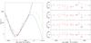Fig. 3 Left panel: dips’s arrival time delays versus time. The magenta, blue, black , and green curves are the best-fit curves obtained using the linear+quadratic (LQ), linear+sinusoidal (LS), linear+quadratic+sinusoidal (LQS), and linear+sinusoidal function taking into account a possible eccentricity (LSe), respectively. Right panel: observed minus calculated delays in units of seconds. The residuals, from the top to the bottom, correspond to the LQC, LS, LQS, and LSe function, respectively.

Initially we fitted the delays with a quadratic function

$\mathit{y}\mathrm{\left(}\mathit{t}\mathrm{\right)}\mathrm{=}\mathit{a}\mathrm{+}\mathit{bt}\mathrm{+}\mathit{c}{\mathit{t}}^{\mathrm{2}}\mathit{,}$where t is the time in days with respect to T₀, a = ΔT₀ is the correction to T₀ in units of seconds, b = ΔP/P₀ in units of s d^-1 with ΔP the correction to the orbital period, and finally, c = 1 / 2Ṗ/P₀ in units of s d^-2, with Ṗ, that is the orbital period derivative. The quadratic form does not fit the data, we obtained χ²(d.o.f.) of 194.6(24). Here, and in the following, we scaled the uncertainties in the parameters by a factor $\sqrt{{\mathit{\chi }}_{\mathrm{red}}^{\mathrm{2}}}$ to take a value of ${\mathit{\chi }}_{\mathrm{red}}^{\mathrm{2}}$ of the best-fit model larger than 1 into account. The best-fit parameters are shown in the second column of Table 4. The corresponding quadratic ephemeris (hereafter LQ ephemeris) is $\begin{array}{ccc}{\mathit{T}}_{\mathrm{dip}}\mathrm{\left(}\mathit{N}\mathrm{\right)}& \mathrm{=}& \mathrm{MJD}\mathrm{\left(}\mathrm{TDB}\mathrm{\right)}\mathrm{50}\hspace{0.17em}\mathrm{123.0096}\mathrm{\left(}\mathrm{3}\mathrm{\right)}\mathrm{+}\frac{\mathrm{3000.65094}\mathrm{\left(}\mathrm{14}\mathrm{\right)}}{\mathrm{86}\hspace{0.17em}\mathrm{400}}\mathit{N}\\ & & \mathrm{+}\mathrm{2.37}\mathrm{\left(}\mathrm{12}\mathrm{\right)}\mathrm{\times }{\mathrm{10}}^{-13}{\mathit{N}}^{\mathrm{2}}\mathit{,}\end{array}$(1)where N is the number of cycles, 50 123.0096(3) MJD is the new Epoch of reference, the revised orbital period is P = 3000.65094(14) s, and the orbital period derivative obtained from the quadratic term is Ṗ = 1.36(7) × 10^-11 s/s. The obtained quadratic ephemeris is compatible with that reported by Hu et al. (2008). We show the best-fit curve in Fig. 3 (left panel) and the corresponding residuals in units of seconds in Fig. 3 (right panel, upper plot).

As we obtained a large value of the χ², we fitted the delays vs. time adding a cubic term to the previous parabolic function, i.e.

$\mathit{y}\mathrm{\left(}\mathit{t}\mathrm{\right)}\mathrm{=}\mathit{a}\mathrm{+}\mathit{bt}\mathrm{+}\mathit{c}{\mathit{t}}^{\mathrm{2}}\mathrm{+}\mathrm{d}{\mathit{t}}^{\mathrm{3}}\mathit{,}$where a, b and c are above defined whilst the cubic term, d, is defined as $\begin{array}{c}{}_{\mathrm{¨}}\\ \mathit{P}\end{array}\mathit{/}\mathrm{\left(}\mathrm{6}{\mathit{P}}_{\mathrm{0}}\mathrm{\right)}\mathit{,}$ and $\begin{array}{c}{\mathrm{¨}}_{}\\ \mathit{P}\end{array}$ indicates the temporal derivative of the orbital period derivative. Fitting with a cubic function, we obtained a χ²(d.o.f.) of 92.4(23) with a Δχ² of 101.2 and an F-test probability of chance improvement of 4.2 × 10^-5 with respect to the quadratic form. The best-fit values are shown in the third column of Table 4. The corresponding ephemeris (hereafter LQC ephemeris) is 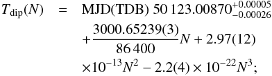$\begin{array}{ccc}{\mathit{T}}_{\mathrm{dip}}\mathrm{\left(}\mathit{N}\mathrm{\right)}& \mathrm{=}& \mathrm{MJD}\mathrm{\left(}\mathrm{TDB}\mathrm{\right)}\mathrm{50}\hspace{0.17em}\mathrm{123.0087}{\mathrm{0}}_{-0.00026}^{\mathrm{+}\mathrm{0.00005}}\\ & & \mathrm{+}\frac{\mathrm{3000.65239}\mathrm{\left(}\mathrm{3}\mathrm{\right)}}{\mathrm{86}\hspace{0.17em}\mathrm{400}}\mathit{N}\mathrm{+}\mathrm{2.97}\mathrm{\left(}\mathrm{12}\mathrm{\right)}\\ & & \mathrm{\times }{\mathrm{10}}^{-13}{\mathit{N}}^{\mathrm{2}}\mathrm{-}\mathrm{2.2}\mathrm{\left(}\mathrm{4}\mathrm{\right)}\mathrm{\times }{\mathrm{10}}^{-22}{\mathit{N}}^{\mathrm{3}}\mathrm{;}\end{array}$(2)in this case we find an orbital period derivative of 1.71(7) × 10^-11 s/s and its derivative is $\begin{array}{c}{}_{\mathrm{¨}}\\ \mathit{P}\end{array}\mathrm{=}\mathrm{-}\mathrm{3.8}\mathrm{\left(}\mathrm{0.7}\mathrm{\right)}\mathrm{\times }{\mathrm{10}}^{-20}$ s/s².

We also fitted the delays using a linear plus a sinusoidal function having the following terms $\begin{array}{ccc}\mathit{y}\mathrm{\left(}\mathit{t}\mathrm{\right)}\mathrm{=}\mathit{a}\mathrm{+}\mathit{bt}\mathrm{+}\mathit{A}\sin \left[\frac{\mathrm{2}\mathit{\pi }}{{\mathit{P}}_{\mathrm{mod}}}\mathrm{(}\mathit{t}\mathrm{-}{\mathit{t}}_{\mathit{\phi }}\mathrm{)}\right]\mathit{,}& & \end{array}$(3)where a and b are defined as above, A is the amplitude of the sinusoidal function in seconds, P_mod is the period of the sine function in days, and, finally, t_φ is the time in days referred to T₀ at which the sinusoidal function is null. We obtained a value of χ²(d.o.f.) of 63.7(22) with a Δχ² of 131 with respect to the quadratic form. The best-fit parameters are shown in the fourth column of Table 4. The best-fit function is indicated with a blue curve in Fig. 3 (left panel) and the corresponding residuals are shown in Fig. 3 (right panel, the second plot from the top). The residuals are flatter than those obtained in the previous case. Using the sinusoidal function, the dip time obtained from the OSO-8 observation is distant ~200 s from the expected value. The corresponding ephemeris (hereafter LS ephemeris) is $\begin{array}{ccc}{\mathit{T}}_{\mathrm{dip}}\mathrm{\left(}\mathit{N}\mathrm{\right)}& \mathrm{=}& \mathrm{MJD}\mathrm{\left(}\mathrm{TDB}\mathrm{\right)}\mathrm{50}\hspace{0.17em}\mathrm{123.01549}\mathrm{\left(}\mathrm{18}\mathrm{\right)}\\ & & \mathrm{+}\frac{\mathrm{3000.6496}\mathrm{\left(}\mathrm{8}\mathrm{\right)}}{\mathrm{86}\hspace{0.17em}\mathrm{400}}\mathit{N}\mathrm{+}\mathit{A}\sin \left[\frac{\mathrm{2}\mathit{\pi }}{{\mathit{N}}_{\mathrm{mod}}}\mathit{N}\mathrm{-}\mathit{\phi }\right]\mathit{,}\end{array}$(4)where N_mod = P_mod/P₀ = 587 659.53 ± 97 351.67 and φ = 2πt_φ/P_mod = with P_mod = 55.9 ± 9.3 yr. This functional form significantly improves the fit, even though it does not take the possible presence of an orbital period derivative into account.

We added a quadratic term to take the possible presence of an orbital period derivative and fitted the delays into account, using the function $\begin{array}{ccc}\mathit{y}\mathrm{\left(}\mathit{t}\mathrm{\right)}\mathrm{=}\mathit{a}\mathrm{+}\mathit{bt}\mathrm{+}\mathit{c}{\mathit{t}}^{\mathrm{2}}\mathrm{+}\mathit{A}\sin \left[\frac{\mathrm{2}\mathit{\pi }}{{\mathit{P}}_{\mathrm{mod}}}\mathrm{(}\mathit{t}\mathrm{-}{\mathit{t}}_{\mathit{\phi }}\mathrm{)}\right]\mathit{.}& & \end{array}$(5)We obtained a value of χ²(d.o.f.) of 39.4(21) and a F-test probability of chance improvement with respect to the LS ephemeris of 1.7 × 10^-3. The best-fit parameters are shown in the fifth column of Table 4. The best-fit function is indicated with a black curve in Fig. 3 (left panel) and the corresponding residuals are shown in Fig. 3 (right panel, the third plot from the top). The corresponding linear+quadratic+sinusoidal ephemeris (hereafter LQS ephemeris) is $\begin{array}{ccc}{\mathit{T}}_{\mathrm{dip}}\mathrm{\left(}\mathit{N}\mathrm{\right)}& \mathrm{=}& \mathrm{MJD}\mathrm{\left(}\mathrm{TDB}\mathrm{\right)}\mathrm{50}\hspace{0.17em}\mathrm{123.0089}\mathrm{\left(}\mathrm{3}\mathrm{\right)}\mathrm{+}\frac{\mathrm{3000.65126}\mathrm{\left(}\mathrm{10}\mathrm{\right)}}{\mathrm{86}\hspace{0.17em}\mathrm{400}}\mathit{N}\\ & & \mathrm{+}\mathrm{2.50}\mathrm{\left(}\mathrm{12}\mathrm{\right)}\mathrm{\times }{\mathrm{10}}^{-13}{\mathit{N}}^{\mathrm{2}}\mathrm{+}\mathit{A}\sin \left[\frac{\mathrm{2}\mathit{\pi }}{{\mathit{N}}_{\mathrm{mod}}}\mathit{N}\mathrm{-}\mathit{\phi }\right]\mathit{,}\end{array}$(6)with N_mod = 267 837.87 ± 21 652.90 and φ = 0.92 ± 0.16. The corresponding orbital period derivative is Ṗ = 1.44(7) × 10^-11 s/s and the period of the modulation is P_mod = 25.5 ± 2.1 yr.

Our analysis of the delays suggests that a quadratic or a quadratic plus a cubic term do not fit the delays. A better fit is obtained using a sinusoidal function with a period close to 20 000 d and, finally, adopting a sinusoidal plus a quadratic term, we obtain the best fit of the delays. In this latter case, the sinusoidal function has a period of 9300 d, about half of that obtained using only the sinusoidal function. Moreover, the orbital period derivative Ṗ = 1.44(7) × 10^-11 s/s (compatible with Ṗ = 1.5(3) × 10^-11 s/s obtained by Hu et al. 2008) is extremely high to be explained by a conservative mass transfer and loss of angular momentum from the binary system for gravitational radiation (see next section). This awkward result can be bypassed if the quadratic term is merely an approximation of a further sinusoidal function with a larger orbital period with respect to 9300 d.

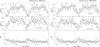Fig. 4 Folded RXTE/ASM light curve of XB 1916-053 in the 3–5 and 5–12.2 keV energy range (top and middle panels). The corresponding hardness ratios (HRs) are plotted in the bottom panels. The left and right plots show the folded RXTE/ASM light curve using the ephemeris discussed by Hu et al. (2008) and LQ ephemeris (Eq. (1)) shown in the Sect. 3, respectively. Each phase-bin is about 50 s.

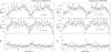Fig. 5 Left and right plots: folded RXTE/ASM light curve using LQC ephemeris (Eq. (2)) and LS ephemeris (Eq. (4)), respectively. Each phase-bin is about 50 s.

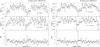Fig. 6 Left and right plots: folded RXTE/ASM light curve using LQS ephemeris (Eq. (6)) and LSe ephemeris (Eq. (8)) with Pmod = 18 600 d, respectively. Each phase-bin is about 50 s.

Under this assumption, the best fit obtained using the LQS ephemeris could be explained using a different scenario, where the quadratic term mimics the fundamental harmonic of a series expansion whilst the sinusoidal term is the first harmonic. This seems also suggested by the best fit obtained using the LS function (Eq. (3)), since we obtain a modulation period, which is almost twice that obtained using the LQS function (Eq. (5)).

If we assume that XB 1916-053 is part of a hierarchical triple system then the measured delays are also affected by the influence of a third body. If the orbits of the third body and of the X-ray binary system around the common centre of mass are slightly elliptical then the delay Δ_DS(t) associated with the Doppler shift can be expressed as $\begin{array}{ccc}{\mathrm{\Delta }}_{\mathrm{DS}}\mathrm{\left(}\mathit{t}\mathrm{\right)}& \mathrm{=}& \mathit{A}\{\sin \mathrm{(}{\mathit{m}}_{\mathit{t}}\mathrm{+}\mathit{\varpi }\mathrm{)}\mathrm{+}\frac{\mathit{e}}{\mathrm{2}}\left[\sin \mathrm{(}\mathrm{2}{\mathit{m}}_{\mathit{t}}\mathrm{+}\mathit{\varpi }\mathrm{)}\mathrm{-}\mathrm{3}\sin \mathrm{\left(}\mathit{\varpi }\mathrm{\right)}\right]\\ & & \mathrm{+}\frac{{\mathit{e}}^{\mathrm{2}}}{\mathrm{4}}\mathrm{\left[}\mathrm{2}\sin \mathrm{\right(}\mathrm{3}{\mathit{m}}_{\mathit{t}}\mathrm{+}\mathit{\varpi }\mathrm{)}\mathrm{-}\sin \mathrm{(}{\mathit{m}}_{\mathit{t}}\mathrm{+}\mathit{\varpi }\mathrm{\left)}\cos \mathrm{\right(}\mathrm{2}{\mathit{m}}_{\mathit{t}}\mathrm{+}\mathrm{1}\mathrm{)}\\ & & \mathrm{-}\mathrm{2}\sin \mathrm{\left(}{\mathit{m}}_{\mathit{t}}\mathrm{\right)}\cos \mathrm{\left(}\mathit{\varpi }\mathrm{\right)}\mathrm{]}\}\mathit{,}\end{array}$(7)where

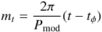${\mathit{m}}_{\mathit{t}}\mathrm{=}\frac{\mathrm{2}\mathit{\pi }}{{\mathit{P}}_{\mathrm{mod}}}\mathrm{(}\mathit{t}\mathrm{-}{\mathit{t}}_{\mathit{\phi }}\mathrm{)}$is the mean anomaly; e is the eccentricity of the orbit; P_mod is the orbital period of both the X-ray binary system and the third body around the common centre of mass; ϖ denotes the periastron angle; t_φ is the passage time at the periastron; and A = asini/c is the projected semi-major axis of the orbit, described by the centre of mass of the X-ray binary system around the centre of mass of the triple system. We neglect third and higher order terms in Eq. (7). Limiting Eq. (7) to the first-order terms, it becomes the expression shown by van der Klis & Bonnet-Bidaud (1984). Then, we fitted the delays using

$\mathit{y}\mathrm{\left(}\mathit{t}\mathrm{\right)}\mathrm{=}\mathit{a}\mathrm{+}\mathit{bt}\mathrm{+}{\mathrm{\Delta }}_{\mathrm{DS}}\mathrm{\left(}\mathit{t}\mathrm{\right)}\mathit{.}$Because the 27 available points do not cover a whole period, we arbitrarily fixed the value of P_mod at 18 600, 17 100, and 20 100 d, which are the best, lower, and upper value of the period obtained from the LQS ephemeris multiplied by a factor of two. The best-fit parameters are shown in Table 4 (Cols. 6–8). The χ²(d.o.f.) are similar for the three adopted periods and the F-test probability of chance improvement with respect to LS function is 4.1 × 10^-2, 1.7 × 10^-2, and 0.9 × 10^-2 for a P_mod value of 17 100, 18 600, and 20 100 d, respectively. In the following, we discuss the case of P_mod = 18 600 d. The best-fit function is indicated with a green curve in Fig. 3 (left panel). The corresponding residuals are shown in Fig. 3 (right panel, lower plot). The corresponding ephemeris (hereafter LSe ephemeris) is $\begin{array}{ccc}{\mathit{T}}_{\mathrm{dip}}\mathrm{\left(}\mathit{N}\mathrm{\right)}& \mathrm{=}& \mathrm{MJD}\mathrm{\left(}\mathrm{TDB}\mathrm{\right)}\mathrm{50}\hspace{0.17em}\mathrm{123.010}\mathrm{\left(}\mathrm{3}\mathrm{\right)}\mathrm{+}\frac{\mathrm{3000.6512}\mathrm{\left(}\mathrm{6}\mathrm{\right)}}{\mathrm{86}\hspace{0.17em}\mathrm{400}}\mathit{N}\\ & & \mathrm{+}{\mathrm{\Delta }}_{\mathrm{DS}}\mathrm{\left(}\mathit{N}\mathrm{\right)}\mathit{.}\end{array}$(8)To verify the robustness of our results, we produced the folded light curves in the 3–5 and 5–12.2 keV energy bands of XB 1916-053 obtained from the All Sky Monitor (ASM) on board RXTE using the ephemerides shown above. We inferred those ephemerides using only pointing observations from which we obtained 27 points spanning from 1978 to 2014, whilst the RXTE/ASM light curves cover from 1996 Sep. 01 to 2011 Oct. 31. We applied the barycentre corrections to the RXTE/ASM events. As a first step, we folded the RXTE/ASM light curves of XB 1916-053 using the LQ ephemeris reported by Hu et al. (2008) and by us (Eq. (1)), adopting 60 phase-bins per period corresponding to ~50 s per bin. The folded light curves and the corresponding hardness ratios (HRs) are shown in Fig. 4. None of the HR show an evident increase at phase zero as we would expect if the ephemerides well define the dip arrival times. This implies that those ephemerides do not correctly predict the dip arrival times contained in the RXTE/ASM light curve. Adopting the LQC ephemeris (Eq. (2)), the maximum value of HR (that is 2.8) is reached at phase 0.1 (see Fig. 5, left panels). Also in this case, the LQC ephemeris does not predict the dip arrival times in the ASM light curves of XB 1916-053. Using the LS ephemeris (Eq. (4)) to fold the light curves, we obtained that the maximum value of HR is reached at phase zero and is close to 3.4 (see Fig. 5, right panels). In contrast, with the LQS ephemeris (Eq. (6)) the maximum value of the HR falls in two phase-bins close to phase zero (see Fig. 6, left panels) and the maximum value of HR is 3.2, which is smaller than the value obtained with the LS ephemeris. Finally, we folded the RXTE/ASM light curves using the LSe ephemeris (Eq. (8)). We show the folded light curves and the corresponding HR in Fig. 6 (right panel). In this last case the maximum value of the HR falls in only one phase bin at phase zero and the maximum value of the HR is about 4.5.

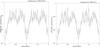Fig. 7 Folded RXTE/ASM light curve of XB 1916-053 selecting the events from SSC1 and SSC2. No energy filter is applied. Each phase-bin correspond to 75 s. Left panel: folded light curve using the LQS ephemeris (Eq. (6)). Right panel: folded light curve using the LSe ephemeris (Eq. (8)).

We also folded the RXTE/ASM light curve (not filtered in energy) using the LQS and LSe ephemerides once we selected the events from the Scanning Shadow Cameras (SSCs) 1 and 2. Adopting 40 phase-bins per period (that is each bin is 75 s), the folded light curves are very similar (see Fig. 7), indicating that the two ephemerides are statistically equivalent. The dip is clearly observed at phase zero, the ASM count rate is reduced during the dip of 60% with respect to the persistent emission. Finally, the goodness of the two ephemerides allows us to observe the presence of a secondary dip at phase 0.55, which is typically observed in several dipping sources (see Grindlay 1989, for XB 1916-053).

4. Discussion

From the study of the 27 dip arrival times obtained from the pointed observations of XB 1916-053 and of the RXTE/ASM light curves, we find that the quadratic and cubic ephemerides do not correctly predict the dip arrival times on a long time span; whilst to well fit the delays, we need to use a function that contains at least linear and sinusoidal terms (LS ephemeris, see Eq. (4)). The addition of a quadratic term to the LS ephemeris (Eq. (6)) gives a probability of chance improvement obtained with a F-test of 1.7 × 10^-3 with respect to the LS ephemeris. Finally, using the ephemeris shown in Eq. (8), the probability of chance improvement, also with respect to the LS ephemeris, is 1.7 × 10^-2. The LQS and LSe ephemerides paint two different physical scenarios for XB 1916-053. In the first case the orbital period derivative of the X-ray binary system is Ṗ = 1.44(7) × 10^-11 s/s and the observed delays associated with the dip arrival times are affected by a relatively low-amplitude (~130 s) sinusoidal modulation with a period close to 26 yr. In the second case the orbital period derivative is fixed to zero and the modulation of the delays is solely sinusoidal with an amplitude of ~550 s and an orbital period close to 51 yr. We explain in the following the sinusoidal modulation for both the scenarios, assuming the presence of a third body forming a hierarchical triple system with XB 1916-053, which alters the observed dip arrival times.

We start by discussing the plausible values of the companion star mass M₂. We know that the companion star is a degenerate star and its radius R₂ has to be equal to its Roche lobe radius R_L2 since the binary system is in the Roche lobe overflow (RLOF) regime. Rearranging the Eq. (3.3.15) in Shapiro & Teukolsky (1983), the mass-radius relation for a degenerate star can be written as

$\frac{{\mathit{R}}_{\mathrm{2}}}{{\mathit{R}}_{\mathrm{\odot }}}\mathrm{=}\mathrm{0.04}{\left(\frac{\mathit{Z}}{\mathit{A}}\right)}^{\mathrm{5}\mathit{/}\mathrm{3}}{\left(\frac{{\mathit{M}}_{\mathrm{2}}}{{\mathit{M}}_{\mathrm{\odot }}}\right)}^{\mathrm{-}\mathrm{1}\mathit{/}\mathrm{3}}\mathrm{=}\mathrm{0.0126}\mathrm{(}\mathrm{1}\mathrm{+}\mathit{X}{\mathrm{)}}^{\mathrm{5}\mathit{/}\mathrm{3}}{\mathit{m}}_{\mathrm{2}}^{\mathrm{-}\mathrm{1}\mathit{/}\mathrm{3}}\mathit{,}$where Z and A are the atomic number and the atomic weight of the matter composing the star, and where we assumed that the matter is only composed of hydrogen and helium. The factor Z/A is the average of Z/A for matter composed of hydrogen and helium, X is the fraction of hydrogen in the star and, finally, m₂ is the companion star mass in units of solar mass. This equation has to be corrected for the thermal bloating factor f, which is the ratio of the companion star radius to the radius of a star with the same mass and composition, that is completely degenerate and supported only by the Fermi pressure of the electrons; then the factor f is >1. The Roche lobe radius of the companion star can be written as

${\mathit{R}}_{\mathit{L}\mathrm{2}}\mathrm{=}\mathrm{0.46224}\mathit{a}{\left(\frac{{\mathit{m}}_{\mathrm{2}}}{{\mathit{m}}_{\mathrm{1}}\mathrm{+}{\mathit{m}}_{\mathrm{2}}}\right)}^{\mathrm{1}\mathit{/}\mathrm{3}}\mathit{,}$where a is the orbital separation of the binary system and m₁ is the neutron star (NS) mass in unit of solar mass. We can write a in terms of the orbital period P, m₁, and m₂, using Kepler’s third law. Combining the last two equations and Kepler’s third law, we obtain $\begin{array}{ccc}{\mathit{m}}_{\mathrm{2}}\mathrm{=}\mathrm{0.0151}\mathrm{(}\mathrm{1}\mathrm{+}\mathit{X}{\mathrm{)}}^{\mathrm{5}\mathit{/}\mathrm{2}}{\mathit{f}}^{\mathrm{3}\mathit{/}\mathrm{2}}\mathit{.}& & \end{array}$(9)Nelemans et al. (2006), analysing the optical spectrum with the European Southern Observatory Very Large Telescope, detected a He-dominated accretion disc spectrum and suggested direct evidence for a helium donor. The authors found a good match with an LTE model consisting of pure helium plus overabundant nitrogen. For this reason, we assume X = 0 in the rest of the discussion.

The bolometric X-ray flux of XB 1916-053 was estimated by several authors. Galloway et al. (2008), analysing a RXTE/PCA observation of XB 1916-053, determined a persistent flux in the 2.5–25 keV of (3.82 ± 0.04) × 10^-10 erg s^-1 cm^-2. The authors corrected the flux for a bolometric factor c_bol = 1.37 ± 0.09 to estimate the bolometric flux in the 0.1–200 keV energy range, obtaining a bolometric flux of (5.2 ± 0.3) × 10^-10 erg s^-1 cm^-2. Recently, Zhang et al. (2014), analysing a Suzaku observation of XB 1916-053, found a value of F_bol in the 0.1–200 keV energy range between 5.5 × 10^-10 and 6.1 × 10^-10 erg s^-1 cm^-2. Finally, analysing the persistent emission of the source during a BeppoSAX observation, Church et al. (1998) estimated a value of F_bol in the 0.5–200 keV energy range of 6.2 × 10^-10 erg s^-1 cm^-2. Since the RXTE/ASM light curve of XB 1916-053 shows that the count rate of the source is almost constant over more than ten years, we adopt a conservative value for the bolometric flux of (5.5 ± 0.5) × 10^-10 erg s^-1 cm^-2.

The distance d to the source was estimated by Galloway et al. (2008) measuring the peak flux during the photospheric radius expansion (PRE) in type-I X-ray bursts. Equation (8) in Galloway et al. (2008) can be rewritten $\begin{array}{ccc}\mathit{d}& \mathrm{=}& \mathrm{8.32}{\left(\frac{{\mathit{F}}_{\mathrm{pk}\mathit{,}\mathrm{PRE}}}{\mathrm{3}\mathrm{\times }{\mathrm{10}}^{-8}\mathrm{erg}{\mathrm{s}}^{-1}\hspace{0.17em}\mathrm{c}{\mathrm{m}}^{-2}}\right)}^{\mathrm{-}\mathrm{1}\mathit{/}\mathrm{2}}{\mathit{m}}_{\mathrm{1}}^{\mathrm{1}\mathit{/}\mathrm{2}}{\left(\mathrm{1}\mathrm{-}\mathrm{0.296}\frac{{\mathit{m}}_{\mathrm{1}}}{{\mathit{r}}_{\mathrm{PRE}}}\right)}^{\mathrm{1}\mathit{/}\mathrm{4}}\\ & & \mathrm{\times }\mathrm{(}\mathrm{1}\mathrm{+}\mathit{X}{\mathrm{)}}^{\mathrm{-}\mathrm{1}\mathit{/}\mathrm{2}}\mathrm{kpc}\mathit{,}\end{array}$(10)where r_PRE is the photospheric radius of the neutron star in units of 10 km and F_pk,PRE is the flux at the peak of the type-I X-ray burst during the PRE. The authors measured F_pk,PRE = (2.9 ± 0.4) × 10^-8ergs^-1cm^-2 and r_PRE ≃ 1.1 for XB 1916-053 and concluded that the distance to the source is d = 8.9 ± 1.3 kpc (adopting X = 0) for a NS mass of 1.4 M_⊙. The X-ray luminosity can be expressed as L_x = 4πd²F_bol, where we roughly assume that the emitted flux is isotropic. We obtain L_x ≃ 5.2 × 10³⁶ erg s^-1 for a NS mass of 1.4 M_⊙, whilst we find L_x ≃ 6.6 × 10³⁶ erg s^-1 for a massive NS of 2.2 M_⊙.

Rappaport et al. (1987) predicted the X-ray luminosity for highly compact binary systems under the reasonable hypothesis that the main mechanism to lose angular momentum is gravitational radiation. Combining the Eqs. (8) and (13) in their work, we obtain $\begin{array}{ccc}{\mathit{L}}_{\mathrm{x}}\mathrm{\simeq }\frac{\mathrm{5.2}\mathrm{\times }{\mathrm{10}}^{\mathrm{42}}}{\mathrm{1}\mathrm{-}\mathrm{1.5}\mathit{\alpha }\mathrm{(}\mathrm{1}\mathrm{-}\mathit{\beta }\mathrm{)}}{\mathit{m}}_{\mathrm{1}}^{\mathrm{5}\mathit{/}\mathrm{3}}{\mathit{P}}_{\mathrm{m}}^{\mathrm{-}\mathrm{14}\mathit{/}\mathrm{3}}\mathrm{(}\mathrm{1}\mathrm{+}\mathit{X}{\mathrm{)}}^{\mathrm{5}}\mathit{\beta \eta }{\mathit{f}}^{\mathrm{3}}{\mathrm{ergs}}^{-1}\mathit{,}& & \end{array}$(11)where P_m is the orbital period in units of minutes, β is the fraction of matter yielded by the companion star and accreted onto the NS, η is the efficiency for converting gravitational potential energy into X-ray emission, and α is the specific angular momentum carried away by the mass lost from the system, in units of 2πa²/P_orb, where a is the orbital separation (see Rappaport et al. 1982). In Eq. (11) we assume that the NS radius is 10 km. Using the orbital period value of 3000.65 s, assuming η = 1 and a conservative mass transfer scenario (β = 1), we find that L_X ≃ 1.1 × 10³⁵f³ erg s^-1 and L_X ≃ 2.3 × 10³⁵f³ erg s^-1 for a NS mass of 1.4 M_⊙ and 2.2 M_⊙, respectively. Comparing the observed luminosity and the predicted luminosity, we estimate that f = 3.6 ± 0.4 and f = 3.0 ± 0.3 for a NS mass of 1.4 M_⊙ and 2.2 M_⊙, respectively. Substituting the obtained values of f in Eq. (9), we obtain that the companion star mass is M₂ = 0.10 ± 0.02 M_⊙ and M₂ = 0.078 ± 0.012 M_⊙ for a NS mass of 1.4 M_⊙ and 2.2 M_⊙, respectively. The mass ratio q = M₂/M₁ of XB 1916-053 is between 0.036 ± 0.009 and 0.071 ± 0.009.

Hu et al. (2008) inferred the mass ratio of XB 1916-053 from the negative super-hump period and found q ≃ 0.045, which is compatible with our estimated range of values of q. Chou et al. (2001) estimated a value of q ≃ 0.022 using the period of the apsidal precession of the accretion disc of P_prec = 3.9087(8) d. The value of q obtained by Chou et al. (2001) is outside the range that we find.

To estimate the orbital period derivative we use the Eq. (11) shown in Rappaport et al. (1987) that we rewrite as $\begin{array}{ccc}\mathit{Ṗ}\mathrm{\simeq }\frac{\mathrm{1.54}\mathrm{\times }{\mathrm{10}}^{-9}}{\mathrm{1}\mathrm{-}\mathrm{1.5}\mathit{\alpha }\mathrm{(}\mathrm{1}\mathrm{-}\mathit{\beta }\mathrm{)}}{\mathit{m}}_{\mathrm{1}}^{\mathrm{2}\mathit{/}\mathrm{3}}{\mathit{P}}_{\mathrm{m}}^{\mathrm{-}\mathrm{8}\mathit{/}\mathrm{3}}\mathrm{(}\mathrm{1}\mathrm{+}\mathit{X}{\mathrm{)}}^{\mathrm{5}\mathit{/}\mathrm{2}}{\mathit{f}}^{\mathrm{3}\mathit{/}\mathrm{2}}{\mathrm{ss}}^{-1}\mathit{.}& & \end{array}$(12)Using the value of Ṗ ~ 1.44 × 10^-11 s s^-1 (LQS ephemeris) and the orbital period value of 3000.65 s, we find that the thermal bloating factor f is 40 and 32 for a NS mass of 1.4 and 2.2 M_⊙. These values of f are not physically plausible and suggest that, in a conservative mass transfer scenario, the value of the orbital period derivative cannot be that obtained from the LQS ephemeris.

On the other hand, adopting an orbital period of 3000.65 s and a factor f of 3.6 and 3.0 for a NS mass of 1.4 and 2.2 M_⊙ we find Ṗ = (3.9 ± 0.2) × 10^-13 s s^-1 and Ṗ = (3.98 ± 0.15) × 10^-13 s s^-1 for a NS mass of 1.4 M_⊙ and 2.2 M_⊙, respectively. The orbital period derivative normalised to the orbital period is Ṗ/P ≃ 4.2 × 10^-9 yr^-1 and weakly depends on the NS mass. We conclude that the conservative mass transfer scenario with a thermal bloating factor of the companion star between three and four allows us to explain the discrepancy between the predicted and observed X-ray luminosity, but it does not solve the discrepancy between the predicted and measured orbital period derivative obtained from the LQS ephemeris. For this reason, we investigate the non-conservative mass transfer scenario.

Combining the Eqs. (11) and (12), we obtain $\begin{array}{ccc}\frac{{\mathit{L}}_{\mathrm{x}}}{\mathit{Ṗ}}\mathrm{\simeq }\mathrm{3.38}\mathrm{\times }{\mathrm{10}}^{\mathrm{51}}{\mathit{m}}_{\mathrm{1}}{\mathit{P}}_{\mathrm{m}}^{-2}\mathit{\beta }{\mathit{f}}^{\mathrm{3}\mathit{/}\mathrm{2}}\mathit{\eta }{\mathrm{ergs}}^{-1}\mathit{.}& & \end{array}$(13)Adopting L_x ≃ 5.2 × 10³⁶ erg s^-1, Ṗ = 1.44 × 10^-11 s s^-1, P = 3000.65 s and fixing η = 1, we find that βf^{3 / 2} = 0.191 for a NS mass of 1.4 M_⊙. Since f> 1, we expect that more than 81% of the mass yielded by the companion star leaves the system. Furthermore, since the measured values of L_x and Ṗ are positive, the term 1–1.5α(1 − β) in Eqs. (11) and (12) should be positive. Solving for α while taking β< 0.191, we obtain that α< 0.823. Because α is in unit of 2πa²/P_orb, we find that the matter should leave the binary system from a distance from the neutron star of ; the point of ejection in unit of orbital separation is . In the rest of the discussion, we assume that the matter is ejected at the inner Lagrangian point x_L1 of the binary system. We rewrite the Eq. (11) as function of f using the condition βf^{3 / 2} = 0.191. We find $\begin{array}{ccc}{\mathit{L}}_{\mathrm{x}}& \mathrm{\simeq }& \frac{\mathrm{5.2}\mathrm{\times }{\mathrm{10}}^{\mathrm{42}}}{\mathrm{1}\mathrm{-}\mathrm{1.5}\overline{{\mathit{x}}_{\mathit{L}\mathrm{1}}}\mathrm{2}\mathrm{(}\mathrm{1}\mathrm{-}\mathrm{0.191}{\mathit{f}}^{\mathrm{-}\mathrm{3}\mathit{/}\mathrm{2}}\mathrm{)}}{\mathit{m}}_{\mathrm{1}}^{\mathrm{5}\mathit{/}\mathrm{3}}{\mathit{P}}_{\mathrm{m}}^{\mathrm{-}\mathrm{14}\mathit{/}\mathrm{3}}\\ & & \mathrm{\times }\hspace{0.17em}\hspace{0.17em}\mathrm{0.191}{\mathit{f}}^{\mathrm{3}\mathit{/}\mathrm{2}}{\mathrm{ergs}}^{-1}\mathit{,}\end{array}$(14)where $\overline{{\mathit{x}}_{\mathit{L}\mathrm{1}}}$ is the position of the inner Lagrangian point in units of orbital separation. Using Eq. (9) and a NS mass of 1.4 M_⊙, $\overline{{\mathit{x}}_{\mathit{L}\mathrm{1}}}$ can be written as a cubic function of f for values of the thermal bloating factor between 1 and 10. We find

$\overline{{\mathit{x}}_{\mathit{L}\mathrm{1}}}\mathrm{=}\mathrm{0.915}\mathrm{-}\mathrm{6.87}\mathrm{\times }{\mathrm{10}}^{-2}\mathit{f}\mathrm{+}\mathrm{6.61}\mathrm{\times }{\mathrm{10}}^{-3}{\mathit{f}}^{\mathrm{2}}\mathrm{-}\mathrm{2.88}\mathrm{\times }{\mathrm{10}}^{-4}{\mathit{f}}^{\mathrm{3}}\mathit{,}$with an accuracy of 2 × 10^-3. Combining the last equation and Eq. (14), we infer the luminosity as function of f. We show L_x in unit of 10³⁶ erg s^-1 versus f for a NS mass of 1.4 M_⊙ (purple colour) in Fig. 8. Since the observed luminosity for a NS mass of 1.4 M_⊙ is larger than the predicted one for each value of f, also taking the corresponding error into account, we conclude that this specific non-conservative mass transfer scenario fails for a NS mass of 1.4 M_⊙.

Fig. 8 X-ray luminosity of XB 1916-053 in units of 1036 erg s-1 versus the thermal bloating factor f of the companion star. The four curves correspond to different values of the NS mass: purple, green, light blue, and gold colours correspond to a NS mass of 1.4, 2, 2.1, and 2.2 M⊙, respectively. The peaks in the curves are at f ≃ 1.5.

We repeat the same procedure for NS masses of 2, 2.1 and 2.2 M_⊙, finding that the predicted and observed luminosities are only compatible in the case in which the NS mass is ≥2.2 M_⊙. In this case ,we find that βf^{3 / 2} = 0.154, α< 0.784 and

$\overline{{\mathit{x}}_{\mathit{L}\mathrm{1}}}\mathrm{=}\mathrm{0.927}\mathrm{-}\mathrm{6.02}\mathrm{\times }{\mathrm{10}}^{-2}\mathit{f}\mathrm{+}\mathrm{5.66}\mathrm{\times }{\mathrm{10}}^{-3}{\mathit{f}}^{\mathrm{2}}\mathrm{-}\mathrm{2.88}\mathrm{\times }{\mathrm{10}}^{-4}{\mathit{f}}^{\mathrm{3}}\mathit{,}$with an accuracy of 2 × 10^-3. The luminosity for a NS mass of 2.2 M_⊙ (gold colour) is shown in Fig. 8. Furthermore, we plot the orbital period derivative as function of f for a NS mass of 2.1 M_⊙ (brown colour) and 2.2 M_⊙ (purple colour) in Fig. 9. We note that only for a NS mass of 2.2 M_⊙ the predicted and measured Ṗ are compatible for f ≃ 1.5. We conclude that this non-conservative mass transfer scenario predicts the observed values of luminosity and orbital period derivative only for NS masses larger than 2.2 M_⊙. For a NS mass of 2.2 M_⊙, the companion star has a mass of 0.028 M_⊙ and β is close to 0.084, which is more than 90% of the matter, yielded from the companion star, that leaves the binary system.

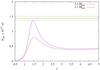Fig. 9 Orbital period derivative of XB 1916-053 in units of 10-11 s s-1 versus the thermal bloating factor f of the companion star. The brown and purple curves are obtained using a NS mass of 2.1 and 2.2 M⊙. The red and green lines indicate the best-fit value and the values at 68% confidence level of the orbital period derivative obtained from the LQS ephemeris. The purple curve is compatible at 1σ with the measured orbital period derivative for f ≃ 1.5.

In this scenario, we suggest that XB 1916-053 could be considered as a possible progenitor of the ultra-compact “Black Widow” pulsars with very low-mass companions. Benvenuto et al. (2012) proposed that a binary system with an initial orbital period of 0.8 d, composed of a 1.4 M_⊙ NS and a companion star mass of 2 M_⊙, evolves in ~6.5 Gyr forming a binary system that well fits the known orbital parameters of the black widow millisecond pulsar PSR J1719-1438. We note that the same evolutive path fits the orbital parameters of XB 1916-053 at ~5 Gyr from the initial time. At 5 Gyr, the predicted orbital period is 0.035 d, the predicted companion star mass is 0.03 M_⊙, the NS mass is slightly larger than 2.2 M_⊙ (Benvenuto, priv. comm.) and the companion star is helium dominated. These values are very similar to those of XB 1916-053 shown in this work for a non-conservative mass transfer scenario, although a discrepancy between our estimation of $\dot{{\mathit{M}}_{\mathrm{2}}}\mathrm{~}\mathrm{4.1}\mathrm{\times }{\mathrm{10}}^{-9}$M_⊙ yr^-1 and the value suggested by Benvenuto et al. (2012) at 5 Gyr (~10^-10M_⊙ yr^-1) is present. Furthermore, we note that as the spin period of PSR J1719-1438 is 5.7 ms (see Bailes et al. 2011, and references therein) the spin period of the NS in XB 1916-053 could also be extremely short. Indeed, Galloway et al. (2001) interpreted the asymptotic frequency of the coherent burst oscillations in terms of a decoupled surface burning layer and suggested that the NS could have a spin period around 3.7 ms.

Nevertheless, we note that our solution for a non-conservative mass transfer scenario is not supported by a robust physical mechanism to explain the large quantity of matter ejected from the inner Lagrangian point. To date, only two physical mechanisms are known to be able to eject the transferred matter partially (or totally) . The first mechanism predicts that when a super-Eddington mass transfer occurs, the X-ray luminosity has to be at the Eddington limit. Then, the radiation pressure from the compact object pushes away part of the transferred matter from the binary system. This mechanism was recently invoked to explain the large orbital period derivative measured in the accretion disc corona (ADC) source X1822-371 by Burderi et al. (2010), Iaria et al. (2013), and Iaria et al. (2015). However, this mechanism cannot be applied in the case of XB 1916-053 because type-I X-ray bursts are observed in the light curve of the source (see e.g. Fig. 2), whilst the stable burning sets in at high accretion rate values that are comparable to the Eddington limit (see Bildsten 2000, and references therein). Consequently, the mass transfer rate cannot be super-Eddington and this mechanism cannot justify a non-conservative mass transfer scenario. The second mechanism supposes that the X-ray binary system is a transient source and during the X-ray quiescence it is ejecting the transferred matter from the inner Lagrangian point due to the radiation pressure of the magneto-dipole rotator emission. This mechanism, which we call radio ejection after Burderi et al. (2001), was proposed by Di Salvo et al. (2008) to explain the large orbital period derivative measured in SAX J1808.4–3658. However, this mechanism also fails to explain our results because XB 1916-053 is a persistent X-ray source.

Finally, we discuss the sinusoidal modulation observed in the LQS and LSe ephemerides. If we assume a conservative mass transfer scenario, the predicted orbital period derivative is close to 4 × 10^-13 s s^-1 independent of the NS mass. Then we added a quadratic term to the LSe ephemeris to take the predicted value into account. We fitted again the delays using the relation

$\mathit{y}\mathrm{\left(}\mathit{t}\mathrm{\right)}\mathrm{=}\mathit{a}\mathrm{+}\mathit{bt}\mathrm{+}\mathit{c}{\mathit{t}}^{\mathrm{2}}\mathrm{+}{\mathrm{\Delta }}_{\mathrm{DS}}\mathrm{\left(}\mathit{t}\mathrm{\right)}\mathit{,}$where the term c is fixed to 5 × 10^-7 s/d². The fit parameters are reported in Table 5. We note that the addition of the quadratic term does not significantly change the best-fit parameters.

An explanation of the sinusoidal modulation obtained from the LSe ephemeris could be the presence of a third body gravitationally bound to the X-ray binary system. Assuming the existence of a third body of mass M₃, the binary system XB 1916-053 orbits around the new centre of mass (CM) of the triple system. The distance of XB 1916-053 from the new CM is given by a_x = a_binsini = Ac, where i is the inclination angle of the orbit with respect to the line of sight, A is the amplitude of the sinusoidal function obtained from the ephemeris of Eq. (8), and c is the light speed. We obtained a_x = (1.60 ± 0.13) × 10¹³ cm for P_mod = 18 600 d. We can write the mass function of the triple system as

$\frac{{\mathit{M}}_{\mathrm{3}}\sin \mathit{i}}{\mathrm{(}{\mathit{M}}_{\mathrm{3}}\mathrm{+}{\mathit{M}}_{\mathrm{bin}}{\mathrm{)}}^{\mathrm{2}\mathit{/}\mathrm{3}}}\mathrm{=}{\left(\frac{\mathrm{4}{\mathit{\pi }}^{\mathrm{2}}}{\mathit{G}}\right)}^{\mathrm{1}\mathit{/}\mathrm{3}}\frac{{\mathit{a}}_{\mathrm{x}}}{{\mathit{P}}_{\mathrm{mod}}^{\mathrm{2}\mathit{/}\mathrm{3}}}\mathit{,}$where M₃ is the third body mass, M_bin the binary system mass, and finally, P_mod is the orbital period of XB 1916-053 around the CM of the triple system. Substituting the values of M_bin, P_mod, a_x, and assuming an inclination angle for the source of 70°, we find that m₃ is ~0.10 M_⊙ and ~0.14 M_⊙ for a NS mass of 1.4 M_⊙ and 2.2 M_⊙, respectively. We used also P_mod of 17 100 and 20 100 d finding that the values of m₃ are substantially independent of the value of P_mod.

For a non-conservative mass transfer scenario, we discuss the sinusoidal modulation obtained from the LQS ephemeris assuming a NS mass of 2.2 M_⊙. In this case we find that a_x = (3.9 ± 0.5) × 10¹² cm and m₃ ~ 0.055M_⊙ for an inclination angle of 70°.

5. Conclusions

We have systematically analysed all the historically reported X-ray light curves of XB 1916-053, which span 37 years. We find that the previously suggested quadratic ephemeris for this source no longer fits the dip arrival times.

We studied the conservative mass transfer scenario of the system, finding that the thermal bloating factor of the degenerate companion star is 3.6 and 3 for a NS mass of 1.4 and 2.2 M_⊙. In this scenario, the predicted and observed luminosity are compatible (~5–7 × 10³⁶ erg s^-1), although the orbital period derivative is a factor of 40 smaller than the value of 1.44 × 10^-11 s s^-1 obtained fitting the delays with a quadratic plus a sinusoidal function (LQS ephemeris). If the conservative mass transfer scenario is correct, we conclude that the modulation of the delays associated with the dip arrivals time are solely due to a sinusoidal modulation caused by a third body orbiting around the binary system. In this case we estimate the third body mass is 0.10 and 0.14 M_⊙ for NS masses of 1.4 and 2.2 M_⊙, respectively. The orbital period of the third body around XB 1916-053 is close to 55 yr and the orbit shows an eccentricity e = 0.28 ± 0.15.

In a non-conservative mass transfer scenario where the mass is ejected away from the inner Lagrangian point, we find that the observed luminosity and the orbital period derivative obtained from the LQS ephemeris are possible only from a NS mass ≥2.2 M_⊙. In this case we obtain that the thermal bloating factor of the degenerate companion star is f ≃ 1.5, the companion star mass is 0.028 M_⊙, and the fraction of matter yielded by the companion star and accreting onto the NS is β = 0.084. In this scenario, the sinusoidal modulation of the delays can be explained by the presence of a third body orbiting around XB 1916-053 with an period of 26 yr. We find that the third body mass is 0.055 M_⊙. Finally, if the non-conservative mass transfer scenario is valid, we suggest that XB 1916-053 and the ultra-compact black widow system PSR J1719-1438 could be two different stages of the same evolutive path discussed by Benvenuto et al. (2012). If it is true, then the age of XB 1916-053 is close to 5 Gyr, whilst PSR J1719-1438 is ~6.5 Gyr old.

Online material

Acknowledgments

This research has made use of data and/or software provided by the High Energy Astrophysics Science Archive Research Center (HEASARC), which is a service of the Astrophysics Science Division at NASA/GSFC and the High Energy Astrophysics Division of the Smithsonian Astrophysical Observatory. We thank the Swift team duty scientists and science planners. The High-Energy Astrophysics Group of Palermo acknowledges support from the Fondo Finalizzato alla Ricerca (FFR) 2012/13, project No. 2012-ATE-0390, founded by the University of Palermo. This work was partially supported by the Regione Autonoma della Sardegna through POR-FSE Sardegna 2007–2013, L.R. 7/2007, Progetti di Ricerca di Base e Orientata, Project N. CRP-60529, and by the INAF/PRIN 2012-6. We also acknowledge financial contribution from the agreement ASI-INAF I/037/12/0. P.R. acknowledges contract ASI-INAF I/004/11/0. A.R. gratefully acknowledges Sardinia Regional Government for the financial support (P.O.R. Sardegna F.S.E. Operational Programme of the Autonomous Region of Sardinia, European Social Fund 2007–2013 – Axis IV Human Resources, Objective l.3, Line of Activity l.3.1.).

References

All Tables

All Figures

	Fig. 1 Chandra/LEG light curves of XB 1916-053 during the two observations performed in 2013, i.e. obsid. 15271 (left) and 15657 (right). The bin time is 64 s. A type-I X-ray burst that occurred during the obsid. 15271.
In the text

	Fig. 2 Suzaku/XIS0 light curve of XB 1916-053 during the long observation on 2014 Oct.
In the text

Fig. 3 Left panel: dips’s arrival time delays versus time. The magenta, blue, black , and green curves are the best-fit curves obtained using the linear+quadratic (LQ), linear+sinusoidal (LS), linear+quadratic+sinusoidal (LQS), and linear+sinusoidal function taking into account a possible eccentricity (LSe), respectively. Right panel: observed minus calculated delays in units of seconds. The residuals, from the top to the bottom, correspond to the LQC, LS, LQS, and LSe function, respectively.

In the text

	Fig. 4 Folded RXTE/ASM light curve of XB 1916-053 in the 3–5 and 5–12.2 keV energy range (top and middle panels). The corresponding hardness ratios (HRs) are plotted in the bottom panels. The left and right plots show the folded RXTE/ASM light curve using the ephemeris discussed by Hu et al. (2008) and LQ ephemeris (Eq. (1)) shown in the Sect. 3, respectively. Each phase-bin is about 50 s.
In the text

	Fig. 5 Left and right plots: folded RXTE/ASM light curve using LQC ephemeris (Eq. (2)) and LS ephemeris (Eq. (4)), respectively. Each phase-bin is about 50 s.
In the text

	Fig. 6 Left and right plots: folded RXTE/ASM light curve using LQS ephemeris (Eq. (6)) and LSe ephemeris (Eq. (8)) with Pmod = 18 600 d, respectively. Each phase-bin is about 50 s.
In the text

	Fig. 7 Folded RXTE/ASM light curve of XB 1916-053 selecting the events from SSC1 and SSC2. No energy filter is applied. Each phase-bin correspond to 75 s. Left panel: folded light curve using the LQS ephemeris (Eq. (6)). Right panel: folded light curve using the LSe ephemeris (Eq. (8)).
In the text

	Fig. 8 X-ray luminosity of XB 1916-053 in units of 1036 erg s-1 versus the thermal bloating factor f of the companion star. The four curves correspond to different values of the NS mass: purple, green, light blue, and gold colours correspond to a NS mass of 1.4, 2, 2.1, and 2.2 M⊙, respectively. The peaks in the curves are at f ≃ 1.5.
In the text

Fig. 9 Orbital period derivative of XB 1916-053 in units of 10-11 s s-1 versus the thermal bloating factor f of the companion star. The brown and purple curves are obtained using a NS mass of 2.1 and 2.2 M⊙. The red and green lines indicate the best-fit value and the values at 68% confidence level of the orbital period derivative obtained from the LQS ephemeris. The purple curve is compatible at 1σ with the measured orbital period derivative for f ≃ 1.5.

In the text

References

- Bailes, M., Bates, S. D., Bhalerao, V., et al. 2011, Science, 333, 1717 [NASA ADS] [CrossRef] [Google Scholar]
- Barret, D., Grindlay, J. E., Strickman, M., & Vedrenne, G. 1996, A&AS, 120, C269 [NASA ADS] [Google Scholar]
- Becker, R. H., Smith, B. W., Swank, J. H., et al. 1977, ApJ, 216, L101 [NASA ADS] [CrossRef] [Google Scholar]
- Benvenuto, O. G., De Vito, M. A., & Horvath, J. E. 2012, ApJ, 753, L33 [NASA ADS] [CrossRef] [Google Scholar]
- Bildsten, L. 2000, in AIP Conf. Ser. 522, eds. S. S. Holt, & W. W. Zhang, 359 [Google Scholar]
- Boirin, L., Parmar, A. N., Barret, D., Paltani, S., & Grindlay, J. E. 2004, A&A, 418, 1061 [NASA ADS] [CrossRef] [EDP Sciences] [Google Scholar]
- Burderi, L., Possenti, A., D’Antona, F., et al. 2001, ApJ, 560, L71 [NASA ADS] [CrossRef] [Google Scholar]
- Burderi, L., Di Salvo, T., Riggio, A., et al. 2010, A&A, 515, A44 [NASA ADS] [CrossRef] [EDP Sciences] [Google Scholar]
- Callanan, P. J., Grindlay, J. E., & Cool, A. M. 1995, PASJ, 47, 153 [NASA ADS] [Google Scholar]
- Chou, Y., Grindlay, J. E., & Bloser, P. F. 2001, ApJ, 549, 1135 [NASA ADS] [CrossRef] [Google Scholar]
- Church, M. J., Dotani, T., BaŁuciŃska-Church, M., et al. 1997, ApJ, 491, 388 [NASA ADS] [CrossRef] [Google Scholar]
- Church, M. J., Parmar, A. N., Balucinska-Church, M., et al. 1998, A&A, 338, 556 [NASA ADS] [Google Scholar]
- Courvoisier, T. J.-L., Walter, R., Beckmann, V., et al. 2003, A&A, 411, L53 [NASA ADS] [CrossRef] [EDP Sciences] [Google Scholar]
- Di Salvo, T., Burderi, L., Riggio, A., Papitto, A., & Menna, M. T. 2008, MNRAS, 389, 1851 [NASA ADS] [CrossRef] [Google Scholar]
- Galloway, D. K., Chakrabarty, D., Muno, M. P., & Savov, P. 2001, ApJ, 549, L85 [NASA ADS] [CrossRef] [Google Scholar]
- Galloway, D. K., Muno, M. P., Hartman, J. M., Psaltis, D., & Chakrabarty, D. 2008, ApJS, 179, 360 [NASA ADS] [CrossRef] [Google Scholar]
- Grindlay, J. E. 1989, in Two Topics in X-Ray Astronomy, Vol. 1: X Ray Binaries. Vol. 2: AGN and the X Ray Background, eds. J. Hunt, & B. Battrick, ESA Spec. Publ., 296, 121 [Google Scholar]
- Grindlay, J. E. 1992, in Frontiers Science Series, eds. Y. Tanaka, & K. Koyama (Tokyo: Universal Academy Press), 69 [Google Scholar]
- Grindlay, J. E., Cohn, H., & Schmidtke, P. 1987, IAU Circ, 4393, 1 [NASA ADS] [Google Scholar]
- Grindlay, J. E., Bailyn, C. D., Cohn, H., et al. 1988, ApJ, 334, L25 [NASA ADS] [CrossRef] [Google Scholar]
- Hu, C.-P., Chou, Y., & Chung, Y.-Y. 2008, ApJ, 680, 1405 [NASA ADS] [CrossRef] [Google Scholar]
- Iaria, R., Di Salvo, T., Lavagetto, G., Robba, N. R., & Burderi, L. 2006, ApJ, 647, 1341 [NASA ADS] [CrossRef] [Google Scholar]
- Iaria, R., Di Salvo, T., D’Aì, A., et al. 2013, A&A, 549, A33 [NASA ADS] [CrossRef] [EDP Sciences] [Google Scholar]
- Iaria, R., Di Salvo, T., Matranga, M., et al. 2015, A&A, 577, A63 [NASA ADS] [CrossRef] [EDP Sciences] [Google Scholar]
- Lund, N., Budtz-Jørgensen, C., Westergaard, N. J., et al. 2003, A&A, 411, L231 [NASA ADS] [CrossRef] [EDP Sciences] [Google Scholar]
- Nelemans, G., Jonker, P. G., & Steeghs, D. 2006, MNRAS, 370, 255 [NASA ADS] [CrossRef] [Google Scholar]
- Paczynski, B., & Sienkiewicz, R. 1981, ApJ, 248, L27 [NASA ADS] [CrossRef] [Google Scholar]
- Priedhorsky, W. C., & Terrell, J. 1984, ApJ, 280, 661 [NASA ADS] [CrossRef] [Google Scholar]
- Rappaport, S., Joss, P. C., & Webbink, R. F. 1982, ApJ, 254, 616 [NASA ADS] [CrossRef] [Google Scholar]
- Rappaport, S., Ma, C. P., Joss, P. C., & Nelson, L. A. 1987, ApJ, 322, 842 [NASA ADS] [CrossRef] [Google Scholar]
- Retter, A., Chou, Y., Bedding, T. R., & Naylor, T. 2002, MNRAS, 330, L37 [NASA ADS] [CrossRef] [Google Scholar]
- Shapiro, S. L., & Teukolsky, S. A. 1983, Black Holes, White Dwarfs, and Neutron Stars: the Physics of Compact Objects (John Wiley VCH) [Google Scholar]
- Smale, A. P., Mason, K. O., White, N. E., & Gottwald, M. 1988, MNRAS, 232, 647 [NASA ADS] [CrossRef] [Google Scholar]
- Smale, A. P., Mason, K. O., Williams, O. R., & Watson, M. G. 1989, PASJ, 41, 607 [NASA ADS] [Google Scholar]
- Swank, J. H., Taam, R. E., & White, N. E. 1984, ApJ, 277, 274 [NASA ADS] [CrossRef] [Google Scholar]
- van der Klis, M., & Bonnet-Bidaud, J. M. 1984, A&A, 135, 155 [NASA ADS] [Google Scholar]
- Walter, F. M., Mason, K. O., Clarke, J. T., et al. 1982, ApJ, 253, L67 [NASA ADS] [CrossRef] [Google Scholar]
- White, N. E. 1989, A&ARv, 1, 85 [NASA ADS] [Google Scholar]
- White, N. E., & Swank, J. H. 1982, ApJ, 253, L61 [NASA ADS] [CrossRef] [Google Scholar]
- Winkler, C., Courvoisier, T. J.-L., Di Cocco, G., et al. 2003, A&A, 411, L1 [NASA ADS] [CrossRef] [EDP Sciences] [Google Scholar]
- Yoshida, K. 1993, Ph.D. Thesis, Tokyo University [Google Scholar]
- Yoshida, K., Inoue, H., Mitsuda, K., Dotani, T., & Makino, F. 1995, PASJ, 47, 141 [NASA ADS] [Google Scholar]
- Zhang, Z., Makishima, K., Sakurai, S., Sasano, M., & Ono, K. 2014, PASJ, 66, 120 [NASA ADS] [Google Scholar]
All Tables
Best-fit parameters of the delays assuming the presence of the third body in eccentric orbit and taking a quadratic term c = 5 × 10⁻⁷ s/d2 into account.