| Issue |
A&A
Volume 686, June 2024
|
|
|---|---|---|
| Article Number | A216 | |
| Number of page(s) | 7 | |
| Section | Stellar structure and evolution | |
| DOI | https://doi.org/10.1051/0004-6361/202449299 | |
| Published online | 13 June 2024 | |
The puzzling orbital residuals of XTE J1710–281: Is a Jovian planet orbiting the binary system?
1
Dipartimento di Fisica e Chimica – Emilio Segrè, Università di Palermo, Via Archirafi 36, 90123 Palermo, Italy
e-mail: This email address is being protected from spambots. You need JavaScript enabled to view it.
2
INAF/IASF Palermo, Via Ugo La Malfa 153, 90146 Palermo, Italy
3
Department of Physics, University of Trento, Via Sommarive 14, 38122 Povo, TN, Italy
4
Dipartimento di Fisica, Università degli Studi di Cagliari, SP Monserrato-Sestu, KM 0.7, Monserrato 09042, Italy
5
INFN, Sezione di Cagliari, Cittadella Universitaria, 09042 Monserrato, CA, Italy
Received:
22
January
2024
Accepted:
12
April
2024
Abstract
Aims. XTE J1710−281 is a transient eclipsing binary system with a period close to 3.28 h that hosts a neutron star. The average eclipse duration is 420 s, and eclipse arrival times reported in the literature span from 1999 to 2017. A previous analysis of the eclipse arrival times using the eclipse timing technique revealed a complex pattern of delays, indicating the presence of three orbital glitches. These glitches correspond to sudden variations in the orbital period and allow for the identification of four distinct epochs, during which the orbital period derivative was estimated to be −1.8 × 10⁻¹² s s−1, 0.07 × 10⁻¹² s s−1, −1.8 × 10⁻¹² s s−1, and 0.09 × 10⁻¹² s s−1, respectively.
Methods. We reanalyzed the 78 eclipse arrival times spanning 18 years utilizing the eclipse timing technique to derive the corresponding delays as a function of time.
Results. We find that the observed delays align well with a fitting model that employs an eccentric sine function characterized by an amplitude of 6.1 ± 0.5 s, an eccentricity of 0.38 ± 0.17, and a period of 17.1 ± 1.5 years. Additionally, we identified the orbital period to be 3.28106345(13) h, with a reference epoch of T0 = 54112.83200(2) MJD. We obtained an upper limit to the orbital period derivative of 3.6 × 10⁻¹³ s s−1.
Conclusions. From the average value of the eclipse duration, we estimate that the companion star has a mass of 0.22 M⊙ for a neutron star mass of 1.4 M⊙ and that the inclination of the source is 78.1−1.2+1.5°. The companion star is in thermal equilibrium. The orbital period derivative is consistent with a conservative mass transfer scenario, where the angular momentum loss due to magnetic braking dominates over gravitational radiation angular momentum loss if the former is present. The eccentric modulation can be explained by a third body with a mass of 2.7 Jovian masses, orbiting with a revolution period close to 17 years and an eccentricity of 0.38.
Key words: eclipses / ephemerides / binaries: eclipsing / stars: neutron / stars: individual: XTE J1710–281
© The Authors 2024
 Open Access article, published by EDP Sciences, under the terms of the Creative Commons Attribution License (https://creativecommons.org/licenses/by/4.0), which permits unrestricted use, distribution, and reproduction in any medium, provided the original work is properly cited.
This article is published in open access under the Subscribe to Open model. This email address is being protected from spambots. You need JavaScript enabled to view it. to support open access publication.
1. Introduction
XTE J1710−281, discovered in 1998 by the Rossi X-ray Timing Explorer (RXTE), is a transient low-mass X-ray binary (LMXB) likely associated with the ROSAT source 1RXS J171012.3−280754 (Markwardt et al. 1998). It exhibits high variability, and numerous Type-I bursts have been documented (Markwardt et al. 2001; Galloway et al. 2008), indicating that the compact object is a neutron star (NS). Galloway et al. (2008) estimated, based on the Type-I bursts, that the distance to the source is 12 kpc, assuming accreting matter with cosmic abundances, or 16 kpc, for accreting matter with helium only.
XTE J1710−281 has an orbital period of 3.28 h (Markwardt et al. 2001) as inferred from analysis of the total eclipses observed in its light curve, which also shows regular dipping phenomena, potentially attributed to occultation from the outer regions of the accretion disk. The presence of dips and total eclipses suggests that the system has an inclination angle between 75° and 80° (Frank et al. 1987). The dips in XTE J1710−281 have been studied by Younes et al. (2009); analyzing XMM-Newton data of the source, they observed that the hydrogen column density is ∼4 × 1021 cm−2 during the persistent emission, from 4 × 1021 cm−2 to 8 × 1023 cm−2 during shallow dips, and ∼1.4 × 1023 cm−2 during deep dips. Analyzing Chandra and Suzaku data, Raman et al. (2018) observed a broad emission line at 0.72 keV, associated with partially ionized iron, and an absorption line in the Fe-K region of the spectrum at 6.6 keV, interpreted as a blend of Fe XIX to Fe XXV transitions.
An accurate study of the eclipses of XTE J1710−281 was performed by Jain & Paul (2011) and Jain et al. (2022), who derived 78 mid-eclipse arrival times by analyzing RXTE, Chandra, Suzaku, XMM-Newton, and AstroSat observations of the source spanning 18 years. The authors estimated the duration of the eclipse to be 420 s on average and, by studying the delays with respect to the orbital cycles, they detected three orbital glitches that current theoretical models cannot explain.
X-ray binaries undergo evolutionary processes driven by various physical mechanisms. One major factor influencing their evolution is mass transfer. This process leads to the redistribution of angular momentum, which impacts the orbital dynamics (van den Heuvel 1994). Moreover, a non-conservative mass transfer can occur as a consequence of different processes, such as radiative evaporation of the secondary star or the expulsion of matter in the form of accretion disk winds, outflows, or jets (Ruderman et al. 1989; Brookshaw & Tavani 1993; Ponti et al. 2012). These mechanisms alter the overall mass content and momentum distribution within the system.
Furthermore, angular momentum lost in the system occurs via two mechanisms: gravitational wave (GR) radiation and magnetic braking (MB) of the tidally locked companion star (CS; Rappaport et al. 1983; Applegate 1992; Applegate & Shaham 1994; Verbunt 1993). These processes directly impact the orbital parameters, contributing to the dynamic evolution of X-ray binaries over time. Consequently, the orbital separation in X-ray binaries can either increase or decrease.
In this study we exploit the mid-eclipse arrival times obtained from Jain & Paul (2011) and Jain et al. (2022) and propose a different interpretation of the orbital residuals of XTE J1710−281. We suggest that the eclipse arrival times are affected by the presence of a third body orbiting the binary system with a mass of 2.7 Jupiter masses and an orbital eccentricity of 0.38.
2. Data analysis
We used the 78 mid-eclipse arrivals times shown by Jain & Paul (2011) and Jain et al. (2022). We started by assuming a reference orbital period of P0 = 3.2810632 h and a reference time of T0 = 54112.83194 modified Julian date (MJD), which corresponds to the mid-eclipse time observed by the RXTE observatory during observation ID 91018-01-02-00 (see Table 1 in Jain & Paul 2011). We inferred the delays corresponding to each eclipse time by taking the fractional part of (Tecl − T0)/P0 and multiplying it by the value of P0 expressed in seconds. We show the eclipse times and the corresponding delays in the top panel of Fig. 1a.
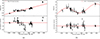 |
Fig. 1. Mid-eclipse time delays for different orbital solutions in units of seconds. (a) Time delays relative to the reference time T0 = 54112.83194 MJD and the orbital period P0 = 3.2810632 h, with best-fit linear function (top panel) and O−C values in units of σ (bottom panel). (b) Time delays based on the reference time T0 = 54112.831977 MJD and the orbital period P0 = 3.28106339 h, with best-fit curve as per Eq. (1) and O−C values in σ units (bottom panel). |
To correct the values of P0 and T0, we fitted the delays with a linear function y = m (t − Ts)+q. The term m = ΔP/P gives the correction to P0, q = ΔT0 is the correction to the reference time T0 and, finally, Ts is fixed to 54112.83194 MJD and corresponds to a temporal shift applied to the eclipse times.
From the fit we obtained a χ2(d.o.f.) of 1298(76), m = 0.0052(3) s days−1 and q = 3.2(5) s. The errors are reported at a 68% (1σ) confidence level. We show the linear best-fit in the top panel of Fig. 1a. The observed minus calculated (O−C) values in units of σ displayed in the bottom panel of Fig. 1a show that the correction is not sufficient to describe the temporal evolution of the source as the delays deviate from the best-fit model up to 10σ. However, a sinusoidal modulation seems to be present in the residuals.
We implemented the corrections from the linear fit by obtaining P0 = 3.281063396(11) h and T0 = 54112.831977(6) MJD and recalculated the delays corresponding to the mid-eclipse times accordingly. We plot the delays versus time in the top panel of Fig. 1b. To fit the delays, we adopted a linear plus sinusoidal function (hereafter LS function) defined as
![Mathematical equation: $$ \begin{aligned} { y} = q + m \;(t-T_{\rm s})+A \sin \left[2\pi \frac{[(t-T_{\rm s})-t_0]}{P_{\rm m}}\right], \end{aligned} $$](/articles/aa/full_html/2024/06/aa49299-24/aa49299-24-eq2.gif) (1)
(1)
where the sinusoidal term takes into account the modulation observed in the O−C values (bottom panel of Fig. 1a). By fitting the data, we found a χ2(d.o.f.) of 253(73) that translates to an F-test probability of chance improvement of 7.4 × 10⁻²⁶ compared to the linear model. The associated errors of the best-fit parameters were scaled by the factor  to take into account a value of the
  of the best-fit model larger than one. We found the following best-fit values: q = 0.16(59) s, m = 0.00129(34) s days−1, A = 6.2(7) s, Pm = 5851(576) days (i.e., 16.0 ± 1.6 years) and t0 = 2285(257) days. By correcting P0 and T0 with the best-fit values of m and q, we obtain T0 = 54112.831979(7) MJD and P0 = 3.28106345(13) h. We show the best-fit function in red in the top panel of Fig. 1b and the corresponding O−C values in units of sigma in the bottom panel. We report the best-fit values of the parameters in the second column of Table 1.
Best-fit parameters.
The ephemeris of the source obtained using the LS function is
![Mathematical equation: $$ \begin{aligned} T_{\rm ecl} =&\mathrm{MJD(TDB)}\; 54112.831979(7) + \frac{3.28106345(13)}{24}N\\&+\frac{6.2(7)}{86400}\sin \left[2\pi \frac{(t-54112.83194)-2285(257)}{5851(576)}\right], \end{aligned} $$](/articles/aa/full_html/2024/06/aa49299-24/aa49299-24-eq5.gif)
where N indicates the orbital cycle and t is expressed in MJD.
We recalculated the delays using the best-fit LS values of T0 and P0. We then fitted the delays with the LS function, ensuring that the parameters q and m had best-fit values compatible with zero. The other fit parameters yield the same best-fit values as reported in the second column of Table 1. In light of the significantly high χ2/d.o.f. value, attributable to residuals that still exhibit clear deviations from the LS model, we considered the possible scenario in which the sinusoidal modulation may be associated with the presence of a third body orbiting around the binary system with eccentricity non-null in a hierarchical triple system.
The determination of the orbital eccentricity was achieved through the application of a numerical solution to Kepler’s equation. The utilized technique involved modeling the delay modulation with an elliptical orbit. The eccentricity, e, was extracted by employing an iterative approach to solve Kepler’s equation. The iterative solution, known as the Newton-Raphson method, facilitated the computation of the eccentric anomaly E = M − e sin E (where M is the mean anomaly), providing a quantitative measure of e. M is defined as π[(t − T0 − Ts)−Tp]/Pm, where Tp is the periastron passage time and Pm the period of the delay modulation.
We call the function adopted to fit the delays “LSe”, which includes a constant term, q, a linear term, m, and an eccentric sinusoidal term. We fitted the data, obtaining a χ2(d.o.f.) of 171.8(71) and a value of the parameter m of 3.3(49)×10−2 s days−1 that is compatible with zero as we expect. To avoid issues related to parameter degeneracy, we fixed the value of m to zero, assessing later its influence on the χ2 value.
By fitting the delays with the LSe model we found a χ2(d.o.f.) of 173(72) and Δχ2 of 80 with respect to the best-fit obtained using the LS function; the F-test probability of chance improvement is 1.85 × 10⁻⁷, corresponding to a significance of 5.2σ, suggests that a non-null eccentricity is required with high statistical significance. The associated errors of the best-fit parameters were scaled by the factor  to take into account a value of
  of the best-fit model larger than one. We obtained q = 1.9(1.4) s, A = 6.1(5) s, Pm = 6249(564) days corresponding to 17.1 ± 1.5 years, Tp = −1261(322) days, e = 0.38(17) and ω = 2.5(4) rad, where ω is the argument of periastron. The delays, the best-fit function, and the corresponding O−C values in units of σ are shown in Fig. 2a (top and bottom panel, respectively). The best-fit values of the parameters are shown in the third column of Table 1. Setting the parameter m equal to zero has little influence on the fit; the F-test probability of chance improvement, leaving the parameter free to vary, is on the order of 0.5.
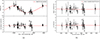 |
Fig. 2. Mid-eclipse time delays for different orbital solutions in units of seconds. (a) Time delays obtained by adopting T0 = 54112.831979 MJD for the reference time and P0 = 3.28106345 as the orbital period (top panel). The best-fit curve (red) is described in the text. O−C values are in units of σ (bottom panel). (b) Time delays obtained by subtracting the eccentric sinusoidal modulation (top panel). The best-fit curve is described by Eq. (2). Corresponding O−C values are in seconds (bottom panel). |
We also explored the correlation of the eccentricity with other parameters but with the parameter m fixed to zero. This correlation is illustrated in Fig. 3, where contour plots for 68% (green), 90% (magenta), and 99% (red) confidence levels are shown across all six panels. Notably, the strongest correlation is observed between eccentricity and parameter q, as well as between the amplitude A of the sinusoidal function and eccentricity e, where e varies within the range of 0.25−0.55. The inclusion of eclipse arrival times distributed over a broader temporal baseline will serve to minimize these correlations, enhancing the reliability of our findings.
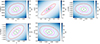 |
Fig. 3. Correlation of eccentricity (e) with other parameters of the LSe function. The correlations are modest, with the most notable observed between parameters q and e. The eccentricity is constrained to be within 0.3 and 0.5 at a 90% confidence level. Contours in green, magenta, and red represent the 68%, 90%, and 99% confidence levels. |
To obtain a constraint on the derivative of the orbital period, Ṗ, we subtracted the best-fit eccentric sinusoidal function from the delays. We then fitted the modified delays using the quadratic function
 (2)
(2)
where c = Ṗ/(2P0) in s days−2. We show the data and the best-fit function in the top panel of Fig. 2b. We obtained the following best-fit values: q = −0.07 ± 0.33 s, m = ( − 0.4 ± 2.0)×10−4 s days−1 and c = (2 ± 9)×10−8 s days−2. Adopting the best-fit value of c we found that Ṗ =(0.7 ± 2.9) × 10−13 s s−1. We show the O−C residuals with respect to this model in the bottom panel of Fig. 2b.
3. Discussion
3.1. The jittered behavior in the eclipse arrival times
In our analysis, we investigated the total eclipse arrival times derived by Jain & Paul (2011) and Jain et al. (2022), who utilized a step-and-ramp function to model the eclipse shape in the light curves of XTE J1710−281. However, it is worth noting that the eclipse shape may vary from one eclipse to another, leading to changes in its ingress/egress and duration times, or solely its ingress/egress time. The ingress, egress, and eclipse durations show a jittered behavior on the order of 15 s in EXO 0748−676 (Wolff et al. 2002), close to 5 s in MXB 1659−298 (Iaria et al. 2018) and up to 10 s in AX J1745.6−2901 (Ponti et al. 2017). We show in the bottom panel of Fig. 2b that the jittered behavior is close to 5 s for XTE J1710−281.
Wolff et al. (2007) proposed that the magnetic activity of the CS can generate extended coronal loops above the CS’s photosphere, accounting for the observed jitters. Furthermore, Ponti et al. (2017) present a different scenario for AX J1745.6−2901, where jitters were observed in the ingress and egress, while the eclipse duration remained relatively constant. They hypothesized that matter ejected from the accretion disk can interact with the CS’s atmosphere, causing displacement and hence delays in the ingress and egress times.
Both scenarios suggest that the presence of magnetic activity and/or the atmosphere of the CS may slightly alter the estimates of the eclipse arrival times. This can increase the reduced chi-square, which may be larger than 1, as obtained for our best-fit model.
3.2. Constraints on the companion star mass
XTE J1710−281 shows total eclipse and dips; therefore, its inclination angle must be between 75° and 80° (see Younes et al. 2009, and references therein). Moreover, the duration of the eclipse ΔTecl is on average about 420 s (Jain & Paul 2011). Using these observational results, we can provide an estimate of the mass ratio q = M2/M1, where M1 and M2 are the masses of the NS and the CS.
Knowing that the eclipse duration is ΔTecl = 420 s, we can estimate the size of the occulted region x (see Fig. 5 in Iaria et al. 2018) by using the expression
 (3)
(3)
where P and a are the orbital period and the orbital separation of the system. The value of x depends on a, which is unknown. The angle, θ, complementary to the inclination angle i of the binary system, can be estimated using the following relationship:
![Mathematical equation: $$ \begin{aligned} \tan \theta = \left[\frac{R_2^2-x^2}{a^2-(R_2^2-x^2)}\right]^{1/2}, \end{aligned} $$](/articles/aa/full_html/2024/06/aa49299-24/aa49299-24-eq10.gif) (4)
(4)
where R2 is the CS radius. In light of the system accreting via the inner Lagrangian point, the CS fills its lobe, resulting in the radius of the CS coinciding with the Roche lobe radius of the CS, which is given by Eggleton (1983)
 (5)
(5)
By substituting Eqs. (3) and (5) into Eq. (4), the angle, θ, depends only on P, which is the known orbital period, on ΔTecl, which is 420 s, and on q, our unknown variable. We show the dependence of the inclination angle on q in Fig. 4.
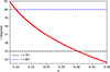 |
Fig. 4. Variation in the inclination angle with the mass ratio, q (red curve), as described by Eq. (4). |
Knowing that the inclination angle of the system ranges between 75° and 80°, we deduce that the mass ratio q falls within the range of 0.1−0.3. Assuming a NS mass of 1.4 M⊙, the CS mass ranges between 0.14 M⊙ and 0.43 M⊙ for an inclination angle of 80° and 75°, respectively.
We can estimate the CS mass with further precision using the mass–radius relationship for stars in thermal equilibrium derived from the study of cataclysmic variables in Knigge et al. (2011). Below, we adopt the mass–radius relationship for binary systems with an orbital period greater than 3.18 h (the orbital period of XTE J1710−281 is close to 3.28 h). The relationship is
 (6)
(6)
where Mconv has a value of 0.20 ± 0.02 M⊙ and represents the mass of the convective region of the CS. This region fills its Roche lobe, RL2, so we can assume that R2 = RL2. Since we estimated that q is between 0.1 and 0.3, we can use the expression for the Roche lobe radius proposed by Paczyński (1971). Combining the expression for the Roche lobe radius with Kepler’s third law, we find that
 (7)
(7)
where m2 is the CS mass in units of solar masses, and Ph is the orbital period in hours. Combining Eqs. (6) and (7), we find M2 = 0.22 ± 0.07 M⊙.
Assuming a NS mass of 1.4 M⊙, we infer that q = 0.16 ± 0.05 corresponds to an inclination angle of  . For a NS mass of 2 M⊙ we obtain q = 0.11 ± 0.03 corresponding to an inclination angle of
  . Using Kepler’s third law, we estimate that the orbital separation of XTE J1710−281 is a = 9.1 × 1010 cm for an inclination angle of 78°, M1 = 1.4 M⊙, and M2 = 0.22 M⊙.
3.3. Self-consistence test for the thermal equilibrium of the CS
We can use the bolometric X-ray luminosity of the source to estimate whether the CS is in thermal equilibrium. To do this, we imposed that the Kelvin-Helmholtz timescale, τKH (corresponding to the characteristic time that a star takes to reach thermal equilibrium), is equal to or less than the mass transfer timescale, τṀ. The Kelvin-Helmholtz timescale is given by the expression
 (8)
(8)
(Verbunt 1993). Adopting the mass-luminosity relation for M-type stars proposed by Neece (1984) and given by the expression L2/L⊙ = 0.231(M2/M⊙)2.61, along with the mass–radius relation from Eq. (6), we obtain  year. The mass-transfer timescale is given by
 (9)
(9)
where Ṁ2 is the mass transfer rate, G is the gravitational constant, LX is the X-ray bolometric luminosity and RNS is the NS radius. In the last equality of Eq. (9), we imposed that the mass transfer rate is equal to the mass accretion rate in the scenario of conservative mass transfer. This point is further discussed later on. We find that  s for a NS radius of 10 km and a NS mass of 1.4 M⊙.
By imposing that τKH ≤ τṀ, we obtain m2 ≥ (1.28 × 10−38 LX)1/2.3. The unabsorbed luminosity in the 0.2−10 keV energy band of XTE J1710−281, during the persistent emission, was estimated to be LX ≃ 2.4 × 1036 erg s−1 for a distance to the source of 16 kpc (Younes et al. 2009). For this luminosity value, we determine that the CS is in thermal equilibrium when m2 ≥ 0.22, which is the CS mass determined by our calculations.
3.4. The orbital period derivative of XTE J1710–281
Drawing upon theoretical frameworks, the mass-transfer rate Ṁ2 within the context of long-term orbital evolution can be expressed as
 (10)
(10)
where ṁ−8 is the mass transfer rate in units of 10−8 M⊙ yr−1, n is the mass–radius index of the CS, Ṗ−10 is the orbital period derivative in units of 10−10 s s−1 and P5h is the orbital period in units of 5 h (see Burderi et al. 2010, and references therein).
Assuming a conservative mass-transfer Ṁ1 = Ṁ2 and considering a source luminosity of 2 × 1036 erg s−1, in the hypothesis that the observed luminosity is a good tracer of the mass accretion rate ṁ, we find ṁ = 1.7 × 10⁻¹⁰ M⊙ yr−1 for a NS mass of 1.4 M⊙ and a NS radius of 10 km. Consequently, the mass transfer rate is Ṁ2 = −1.7 × 10⁻¹⁰ M⊙ yr−1. Using n = 0.69 (adopted in Eq. (6)), m2 = 0.22 and an orbital period of 3.28 h, we find Ṗ = −1.5 × 10⁻¹³ s s−1. This value is consistent within 1σ with what we obtained from our analysis, that is, Ṗ = (0.7 ± 2.9) × 10−13 s s−1; therefore, we should expect that the binary system is undergoing a contraction of the orbit.
The orbital period change due to the loss of angular momentum can be associated with the emission of GRs and MB. Below, we explore both cases assuming a conservative mass-transfer scenario. The orbital period changes due to GRs is given by the relationship
![Mathematical equation: $$ \begin{aligned} \dot{P}_{\rm grav} =&-1.4\times 10^{-12} m_1 m_2 m_T^{-1/3} P_{\rm 2h}^{-5/3}\nonumber \\&\times [(n-1/3) \times (n+5/3-2q)]\;\; \mathrm{s\,s^{-1}}, \end{aligned} $$](/articles/aa/full_html/2024/06/aa49299-24/aa49299-24-eq21.gif) (11)
(11)
where m1 is the NS mass in units of M⊙, mT is m1 + m2 in units of M⊙, P2h is the orbital period in units of two hours, and q is the mass ratio of the binary system (see di Salvo et al. 2008, and references therein). Using the values of m1, m2, P, and n shown above, we estimate Ṗgrav ≃ −2.8 × 10⁻¹⁴ s s−1.
The estimated mass of the CS is less than 0.3 M⊙. Rappaport et al. (1983) proposed that the MB mechanism might not be active, attributing this to the star being fully convective. The lack of a radiative zone implies losing its magnetic field dipolar structure. If this mechanism is inhibited, the only contribution to the orbital period derivative is related to Ṗgrav. However, both Chen (2017) and Tailo et al. (2018) indicated that the MB mechanism could remain active even in stars with masses below 0.3 M⊙. In such a scenario, we expect the contribution of MB to the orbital period variation to be significant.
The contribution to the orbital period variation related to MB is given by the relation
 (12)
(12)
where  (see Eqs. (2) and (3) in Burderi et al. 2010, and references therein). The gyration radius k is in units of 0.277, and since the CS has a mass of 0.22 M⊙, we adopt a value k = 0.45 as reported by Wadhwa et al. (2024). The parameter f can range between 0.78 and 1.73 because it is model dependent (see the discussion in Burderi et al. 2010), and we estimate TMB for the limit values of f finding that TMB ranges between 5.8 and 29. The corresponding orbital period derivative associated with the MB, ṖMB, is therefore between −8.2 × 10⁻¹³ s s−1 and −1.6 × 10⁻¹³ s s−1. The contribution of the angular momentum loss via GR and MB to the orbital period derivative yields Ṗ between −8.5 × 10⁻¹³ s s−1 and −1.9 × 10⁻¹³ s s−1, still compatible with what is obtained from our analysis adopting TMB = 5.8.
3.5. The hierarchical triple system scenario
From the delays fitting, we obtain that the statistically most significant solution involves a sinusoidal modulation with an eccentricity e of 0.38 ± 0.17 and a modulation period of 17.1 ± 1.5 years. The delay modulation could be caused by a third body orbiting around XTE J1710−281, where the modulation period corresponds to the revolution period of the third body around the binary system. We can estimate the mass of the third body under the assumption that its orbit is co-planar with that of the binary system. We estimate the separation between the center of mass (CM) of the binary system and that of the triple hierarchical system to be ax sin i = Ac, where c represents the speed of light, and A is the amplitude of the modulation; ax sin i = 1.8 × 1011 cm in our case. The mass M3 of the third body is given by
 (13)
(13)
where Mbin is the mass of the binary system, G the gravitational constant and Pm the periodic modulation inferred from the delays fit. For an inclination angle of 78° (we assume that the third body orbit lies on the binary system orbital plane), M1 = 1.4 M⊙ and M2 = 0.22 M⊙, we infer that M3 ≃ 2.7 MJ, where MJ indicates the Jupiter mass. The separation between the third body and the CM of the hierarchical triple system is a3 = ax sin i Mbin/M3 ≃ 1.1 × 1014 cm, corresponding to 7.5 AU, approximately equivalent to a distance similar to that between the Sun and halfway between Jupiter and Saturn. Finally, at the periastron passage, the separation between the CM and the third body is d = ax sin i (1 − e) Mbin/M3 = 7.1 × 1013 cm, a distance significantly exceeding the orbital separation of the binary system, represented by a = 9.1 × 1010 cm.
The existence of third celestial bodies in orbit around binary systems, particularly those containing a compact object, is being increasingly confirmed by recent discoveries. Notable among these findings is the proposed detection of a third body with a mass of approximately 45 MJ (0.043 M⊙) by Iaria et al. (2015, 2021) orbiting the dipping source XB 1916−053. Concurrently, Iaria et al. (2018) have revealed a 22 MJ mass third body orbiting the eclipsing source MXB 1659−298. The precedent for such detections was arguably set by Sigurdsson (1993), who proposed the existence of a sub-Jovian mass planet in orbit around the binary system of the millisecond radio pulsar PSR 1620−26 within the globular cluster M 4. Subsequent Hubble Space Telescope observations allowed this model to be refined, positing the third body as a planet with a mass of 2.5 ± 1.0 MJ in orbit around a binary system of a millisecond pulsar and a white dwarf companion (Sigurdsson et al. 2003).
Bailes et al. (2011) discovered a Jupiter-sized chthonian body composed primarily of carbon and oxygen in a close orbit around the millisecond pulsar PSR J1719−1438, at a distance of 0.004 AU. Such observations are in line with the seminal discovery of planets orbiting PSR 1257+12 Wolszczan & Frail (1992), which has spawned a multitude of hypotheses regarding planetary formation in the vicinity of pulsars.
Podsiadlowski (1993) discussed that planetary bodies associated with NSs are supposed to form during one of three distinct periods: (i) within a protoplanetary disk during the initial star formation (first-generation); (ii) from a fallback disk composed of debris of the supernova explosion (second-generation); (iii) or within an accretion disk that forms from matter transferred to the NS from the CS (third-generation). Planets from the first generation, if they exist, are presumed either to have been destroyed or to have had their trajectories severely altered in the wake of a supernova event. The existence of planets orbiting millisecond pulsars challenges the hypothesis of second-generation formation, as the spin acceleration implies a proximal CS, within an orbital distance of roughly 1 AU, and this would likely perturb planets orbits. This is corroborated by the instance of PSR B1257+12, which is a fully recycled pulsar, implying its companion is a low-mass star and had experienced Roche lobe overflow during its main-sequence life stage, necessitating an orbital proximity not exceeding 1 AU.
Therefore, the prevailing hypothesis for the formation of planets orbiting isolated millisecond pulsars supports the idea of third-generation formation, where planets form from the residual matter of the CS. However, this evolutionary channel clashes with the findings of this study, where we have an X-ray binary system undergoing mass transfer from a main-sequence CS. Similarly, this evolutionary path cannot easily explain the three-body system of the millisecond pulsar PSR 1620−26, where the main CS is a white dwarf. Therefore, one possibility is that these planets are solitary planets that were gravitationally captured by the binary system (Podsiadlowski et al. 1991), which is very unlikely for Galactic field systems. Alternatively, it is possible that these planets emerge from a circumbinary disk, formed from material expelled by the CS during a period of non-conservative mass transfer of the LMXB (Tavani & Brookshaw 1992).
3.6. Limitations of the Applegate mechanism in explaining orbital period modulation in XTE J1710–281
Given that the CS is a low-mass star (0.22 M⊙), we expect its magnetic activity to be intense. However, XTE J1710−281 exhibits persistent emission with mass transfer via Roche lobe overflow, so the luminosity from the outer regions of the accretion disk may overshadow that of the CS in the visible band, hindering a detailed study of the CS Ratti et al. (2010). Consequently, the magnetic properties of the CS in XTE J1710−281 are currently unknown.
Nevertheless, an alternative explanation of the modulation of approximately 17 years observed in the orbital delays could be given by a gravitational coupling of the orbit with variations in the shape of the magnetically active CS. These variations are believed to result from the torque exerted by the magnetic activity associated with a subsurface magnetic field in the CS, interacting with its convective envelope. The convective envelope initiates a periodic exchange of angular momentum between the inner and outer regions of the CS, leading to alterations in its gravitational quadrupole moment (Applegate 1992; Applegate & Shaham 1994).
In this instance, the deduced periodicity of 6249 days and amplitude of 6.1 s translates to an orbital period variation of ΔP/P ≃ 2.2 × 10⁻⁵. Under the reasonable assumption that the CS fills its Roche lobe, and consequently, its radius coincides with the Roche-lobe radius, we can calculate the angular momentum transfer required to induce the observed orbital period change to be approximately ΔJ ≃ 4.8 × 1044 g cm2 s−1.
The non-synchronicity of the companion, expressed by the ratio ΔΩ/Ω, is 6.7 × 10⁻⁵, where Ω is the orbital angular velocity of the binary system and ΔΩ represents the variation in the orbital angular velocity required to induce the change in the orbital period, ΔP. The value of ΔΩ/Ω is obtained assuming that a thin shell of mass, Ms is 10% of the CS mass, where the shell represents the limited mass in the outer part of the star that governs the quadrupole moment. For Ms mass larger than 10%, the angular momentum transfer mechanism ceases to function (Applegate 1992).
The variable part of the CS luminosity necessary to fuel the variations in the gravitational quadrupole is ΔL = 2.9 × 10⁻⁵ L⊙. To estimate the required fraction of the CS luminosity to achieve the observed modulation in the delays, we deduce the CS luminosity using the relationship L/L⊙ = 0.231 (M2/M⊙)2.61, applicable to low-mass stars. We find that L ≃ 4.4 × 10⁻³ L⊙ and ΔL ≃ 0.007. To achieve these brightness variations, we would need a shell mass of 0.7% of the CS mass, while the available budget should be around 10% of the CS’s luminosity. This result appears odd with the model, so we conclude that this is unlikely to be the correct explanation.
4. Conclusions
We used the mid-eclipse times reported by Jain & Paul (2011) and Jain et al. (2022) to offer a different interpretation of the orbital residuals of XTE J1710−281. By fitting the delays, we find a periodic modulation of close to 17 years described by an eccentric sinusoidal modulation with an eccentricity of about 0.38 and an amplitude of 6.1 s.
The likely scenario describing the sinusoidal modulation involves a third body orbiting the binary system with a revolution period of 17 years and an orbital eccentricity of 0.38. From these parameters, we deduce that the mass of the third body is 2.7 MJ. The presence of a third body around a binary system has also been discussed for the eclipsing LMXB MXB 1659−298 (Iaria et al. 2018); this third body has a mass exceeding 21 MJ. Moreover, the presence of a third body has also been considered by Iaria et al. (2015) for the ultra-compact LMXB XB 1916−053; in this case, the mass of the third body would exceed 45 MJ.
It is important to emphasize that the presence of a third orbiting body does not contract or expand the orbital period of a binary system. Indeed, the motion of the third body influences the position of the CM of the binary system, thereby affecting the arrival times of eclipses. The derivative of the orbital period obtained in this work is not affected at zero order by the presence of the third body; it reflects the expected evolution of an LMXB system given by the mass transfer and the loss of angular momentum via MB and gravitational radiation in the case of a conservative mass transfer.
Our interpretation of the results, statistically equivalent to that obtained by Jain et al. (2022), rules out the presence of discontinuities in the derivative of the orbital period, for which, to date, there is no theoretical model for their interpretation. Instead, our result aligns with the evolution of a binary system in which the CS of 0.22 M⊙ is in thermal equilibrium, and conservative mass transfer tends to contract the binary system.
Acknowledgments
The authors acknowledge financial support from PRIN-INAF 2019 with the project “Probing the geometry of accretion: from theory to observations” (PI: Belloni). W.L. conducted this research during, and with the support of, the Italian national inter-university PhD program in Space Science and Technology.
References
- Applegate, J. H. 1992, ApJ, 385, 621 [Google Scholar]
- Applegate, J. H., & Shaham, J. 1994, ApJ, 436, 312 [NASA ADS] [CrossRef] [Google Scholar]
- Bailes, M., Bates, S. D., Bhalerao, V., et al. 2011, Science, 333, 1717 [NASA ADS] [CrossRef] [Google Scholar]
- Brookshaw, L., & Tavani, M. 1993, ApJ, 410, 719 [NASA ADS] [CrossRef] [Google Scholar]
- Burderi, L., Di Salvo, T., Riggio, A., et al. 2010, A&A, 515, A44 [NASA ADS] [CrossRef] [EDP Sciences] [Google Scholar]
- Chen, W.-C. 2017, MNRAS, 464, 4673 [NASA ADS] [CrossRef] [Google Scholar]
- di Salvo, T., Burderi, L., Riggio, A., Papitto, A., & Menna, M. T. 2008, MNRAS, 389, 1851 [NASA ADS] [CrossRef] [Google Scholar]
- Eggleton, P. P. 1983, ApJ, 268, 368 [Google Scholar]
- Frank, J., King, A. R., & Lasota, J. P. 1987, A&A, 178, 137 [NASA ADS] [Google Scholar]
- Galloway, D. K., Muno, M. P., Hartman, J. M., Psaltis, D., & Chakrabarty, D. 2008, ApJS, 179, 360 [NASA ADS] [CrossRef] [Google Scholar]
- Iaria, R., Di Salvo, T., Gambino, A. F., et al. 2015, A&A, 582, A32 [NASA ADS] [CrossRef] [EDP Sciences] [Google Scholar]
- Iaria, R., Gambino, A. F., Di Salvo, T., et al. 2018, MNRAS, 473, 3490 [CrossRef] [Google Scholar]
- Iaria, R., Sanna, A., Di Salvo, T., et al. 2021, A&A, 646, A120 [NASA ADS] [CrossRef] [EDP Sciences] [Google Scholar]
- Jain, C., & Paul, B. 2011, MNRAS, 413, 2 [CrossRef] [Google Scholar]
- Jain, C., Sharma, R., & Paul, B. 2022, MNRAS, 517, 2131 [NASA ADS] [CrossRef] [Google Scholar]
- Knigge, C., Baraffe, I., & Patterson, J. 2011, ApJS, 194, 28 [Google Scholar]
- Markwardt, C. B., Marshall, F. E., Swank, J., & Takeshima, T. 1998, IAU Circ., 6998, 2 [NASA ADS] [Google Scholar]
- Markwardt, C. B., Swank, J. H., & Strohmayer, T. E. 2001, Am. Astron. Soc. Meet. Abstr., 199, 27.04 [NASA ADS] [Google Scholar]
- Neece, G. D. 1984, ApJ, 277, 738 [NASA ADS] [CrossRef] [Google Scholar]
- Paczyński, B. 1971, ARA&A, 9, 183 [Google Scholar]
- Podsiadlowski, P. 1993, in Planets Around Pulsars, eds. J. A. Phillips, S. E. Thorsett, & S. R. Kulkarni, ASP Conf. Ser., 36, 149 [Google Scholar]
- Podsiadlowski, P., Pringle, J. E., & Rees, M. J. 1991, Nature, 352, 783 [CrossRef] [Google Scholar]
- Ponti, G., Fender, R. P., Begelman, M. C., et al. 2012, MNRAS, 422, L11 [NASA ADS] [CrossRef] [Google Scholar]
- Ponti, G., De, K., Muñoz-Darias, T., Stella, L., & Nandra, K. 2017, MNRAS, 464, 840 [NASA ADS] [CrossRef] [Google Scholar]
- Raman, G., Maitra, C., & Paul, B. 2018, MNRAS, 477, 5358 [CrossRef] [Google Scholar]
- Rappaport, S., Verbunt, F., & Joss, P. C. 1983, ApJ, 275, 713 [Google Scholar]
- Ratti, E. M., Bassa, C. G., Torres, M. A. P., et al. 2010, MNRAS, 408, 1866 [NASA ADS] [CrossRef] [Google Scholar]
- Ruderman, M., Shaham, J., Tavani, M., & Eichler, D. 1989, ApJ, 343, 292 [NASA ADS] [CrossRef] [Google Scholar]
- Sigurdsson, S. 1993, ApJ, 415, L43 [NASA ADS] [CrossRef] [Google Scholar]
- Sigurdsson, S., Richer, H. B., Hansen, B. M., Stairs, I. H., & Thorsett, S. E. 2003, Science, 301, 193 [NASA ADS] [CrossRef] [Google Scholar]
- Tailo, M., D’Antona, F., Burderi, L., et al. 2018, MNRAS, 479, 817 [NASA ADS] [Google Scholar]
- Tavani, M., & Brookshaw, L. 1992, Nature, 356, 320 [NASA ADS] [CrossRef] [Google Scholar]
- van den Heuvel, E. P. J. 1994, Saas-Fee Advanced Course 22: Interacting Binaries, 263 [CrossRef] [Google Scholar]
- Verbunt, F. 1993, ARA&A, 31, 93 [NASA ADS] [CrossRef] [Google Scholar]
- Wadhwa, S. S., Landin, N. R., Kostić, P., et al. 2024, MNRAS, 527, 1 [Google Scholar]
- Wolff, M. T., Hertz, P., Wood, K. S., Ray, P. S., & Bandyopadhyay, R. M. 2002, ApJ, 575, 384 [NASA ADS] [CrossRef] [Google Scholar]
- Wolff, M. T., Wood, K. S., & Ray, P. S. 2007, ApJ, 668, L151 [CrossRef] [Google Scholar]
- Wolszczan, A., & Frail, D. A. 1992, Nature, 355, 145 [CrossRef] [Google Scholar]
- Younes, G., Boirin, L., & Sabra, B. 2009, A&A, 502, 905 [NASA ADS] [CrossRef] [EDP Sciences] [Google Scholar]
All Tables
All Figures
|
Fig. 1. Mid-eclipse time delays for different orbital solutions in units of seconds. (a) Time delays relative to the reference time T0 = 54112.83194 MJD and the orbital period P0 = 3.2810632 h, with best-fit linear function (top panel) and O−C values in units of σ (bottom panel). (b) Time delays based on the reference time T0 = 54112.831977 MJD and the orbital period P0 = 3.28106339 h, with best-fit curve as per Eq. (1) and O−C values in σ units (bottom panel). |
| In the text | |
|
Fig. 2. Mid-eclipse time delays for different orbital solutions in units of seconds. (a) Time delays obtained by adopting T0 = 54112.831979 MJD for the reference time and P0 = 3.28106345 as the orbital period (top panel). The best-fit curve (red) is described in the text. O−C values are in units of σ (bottom panel). (b) Time delays obtained by subtracting the eccentric sinusoidal modulation (top panel). The best-fit curve is described by Eq. (2). Corresponding O−C values are in seconds (bottom panel). |
| In the text | |
|
Fig. 3. Correlation of eccentricity (e) with other parameters of the LSe function. The correlations are modest, with the most notable observed between parameters q and e. The eccentricity is constrained to be within 0.3 and 0.5 at a 90% confidence level. Contours in green, magenta, and red represent the 68%, 90%, and 99% confidence levels. |
| In the text | |
|
Fig. 4. Variation in the inclination angle with the mass ratio, q (red curve), as described by Eq. (4). |
| In the text | |
Current usage metrics show cumulative count of Article Views (full-text article views including HTML views, PDF and ePub downloads, according to the available data) and Abstracts Views on Vision4Press platform.
Data correspond to usage on the plateform after 2015. The current usage metrics is available 48-96 hours after online publication and is updated daily on week days.
Initial download of the metrics may take a while.