© ESO, 2015

1. Introduction

Following the detection of 51 Peg b by Mayor & Queloz (1995) using velocimetry, almost 2000 exoplanets¹ are known as of today (March 10, 2015) and many more candidates are awaiting confirmation (Rowe et al. 2015). Among them, only a few were detected with direct imaging.

The first image of a planetary mass object orbiting a star, 2M1207 b, was obtained by Chauvin et al. (2004) with NaCo at the Very Large Telescope (VLT) and this result has inspired several other discoveries in the last decade (Marois et al. 2008; Lagrange et al. 2009; Rameau et al. 2013). In the first case, the mass ratio was highly favorable as the central star is a brown dwarf (BD). The detection was enabled by the use of an adaptive optics (AO) system in the L′ band and no specific device to attenuate the star, such as a coronagraph, was needed. Later, larger mass ratios became feasible with the improvement of high contrast imaging techniques. For now, the planet with the largest mass ratio with respect to its host star, and for which we have an image, is HD 95086 b with a mass of 5 ± 2 M_Jup around a star of 1.6 M_Sun (Rameau et al. 2013). Conveniently, direct imaging also allows us to collect spectroscopic data if one is able to attenuate the starlight at the location of the planet. Janson et al. (2010) presented the first spatially resolved spectra of HR8799 c still with NaCo. The spectrum covered the 3.88−4.10 μm interval but with a low signal-to-noise ratio. The OSIRIS instrument at Keck II allowed Bowler et al. (2010) and Barman et al. (2011) to obtain spectra of the exoplanet HR8799 b in the K band, sensitive to methane opacity, as well as a spectrum in the H band (Barman et al. 2011). Later, the same instrument provided spectra of the same planet Barman et al. (2015) and of HR8799 c (Konopacky et al. 2013) in the K band at higher resolution (R ~ 4000). Near-infrared (NIR), low-resolution spectra of the planet β Pictoris b (Lagrange et al. 2010) were obtained with GPI (Macintosh et al. 2014) in the J and H bands (Bonnefoy et al. 2014; Chilcote et al. 2015), an instrument tailored for the search of young giant planets.

At the present time, instruments for direct imaging combine AO, coronography, and differential imaging to detect faint planets. The Spectro-Polarimetric High-contrast Exoplanet Research (SPHERE; Beuzit et al. 2008), installed at the VLT, is designed to perform high contrast imaging for detecting young giant planets and for characterizing their atmospheres. SPHERE provides broad- and narrowband photometry and spectroscopy in the NIR range with the InfraRed Dual-band Imager and Spectrograph (IRDIS, Langlois et al. 2010) and the Integral Field Spectrograph (IFS, Claudi et al. 2008), and photometry and polarimetry in the visible range with the Zurich Imaging Polarimeter (ZIMPOL, Schmid et al. 2010).

To directly detect the light from a planet around a star other than the sun, the following conditions have to be met:

• the star-to-planet angular separation must be larger than the angular resolution offered by an 8-m telescope in the NIR (25–50 mas for SPHERE). This restrains the sample of targets to less than 100 pc as well as the minimal physical separation to ≥1 AU.

• the star-to-planet brightness ratio must be smaller than the achievable instrumental contrast, which is typically 10⁵–10⁷ at less than 1′′. Only giant planets can be warm enough at young ages to produce a detectable emission (Burrows et al. 1995; Chabrier et al. 2000). These young extrasolar giant planets (YEGP) are ~10–100 millions years old.

One theoretical challenge is to understand planetary formation mechanisms. Brown dwarf and young extrasolar giant planet are two types of objects almost impossible to differentiate, which are formed in different ways. Proposed mechanisms are gravitational instabilities (Boss 2001), such as stars, without a sufficient mass to start to burn hydrogen or core accretion (Lin & Ida 1997). A precise determination of the luminosity, mass, and age can supply information about the initial entropy of the planet and allows us to identify the formation mechanism (Bonnefoy et al. 2014; Marleau & Cumming 2014).

In parallel, atmospheric models for objects with mass and temperature lower than an M dwarf were developed since the end of the 1990’s. The basic idea is to include some chemistry and other physical processes in a H-He atmosphere to account for the range of pressure temperature expected in such low-mass objects. The models differ in particular by their treatment of dust opacity. This is a crucial component of the models since it was noticed very soon that these atmospheres must contain clouds below T_eff ≃ 2600 K to account for the spectroscopic observations (Tsuji et al. 1996).

The model of Tsuji and collaborators is a direct adaptation of their M dwarf models to BD. Dust grains in the atmosphere are treated through a parametrized model (Tsuji 2002), with three cases. In Case B, the part of the atmosphere where the temperature is lower than the condensation temperature is full of dust. In an opposite case (Case C), dust forms but is immediately removed by precipitation so that it does not contribute to the opacity. The third case, called the unified cloud model, is intermediate between these two extremes with dust present only between the condensation level and a level at a slightly lower temperature T_c.

Marley et al. (2000) proposed a model adapted from solar system planets and using the Ackerman & Marley (2001) cloud model, which is parametrized with a factor f_sed representing the sedimentation efficiency.

The Lyon’s group atmospheric models, DUSTY and COND (Allard et al. 2001) are two cases similar to Tsuji’s B and C cases. BT-Settl (Allard et al. 2003) is a more complex model, which compares condensation, sedimentation, and mixing timescales of dust to define cloud parameters.

Finally, Drift-PHOENIX (Helling et al. 2008) considers microphysical processes (nucleation, condensation, particle growth, sedimentation, and evaporation) to calculate composition, number density, and size distribution of dust particles as a function of atmospheric pressure level.

All these models were used to constrain the main parameters, such as the effective temperature, surface gravity, atmospheric compounds, or radius of the detected planets (Neuhäuser et al. 2005; Marley et al. 2012; Bonnefoy et al. 2013, 2014; Galicher et al. 2014) and to predict abilities of new instruments (Boccaletti et al. 2005; Hanot et al. 2010; Vigan et al. 2010). Most of these models are developed for BD and applied to exoplanets. Although, the radius of exoplanets can be similar to that of BD, they have lower masses. Therefore, the range of surface gravity considered in BD atmospheric models (log (g) > 3.5) does not necessarily cover the entire range expectable for YEGP (log (g) > 2).

Direct imaging of YEGP is characterized by low flux, low signal to noise and low spectral resolution. In that respect, the models that are used to interpret these images should be representative of the level of data quality. For that purpose we specifically developed a model to analyze direct imaging of YEGP for instruments like SPHERE. It is a radiative-convective equilibrium model, assuming thermochemical equilibrium for self -luminous planets in which stellar heating is neglected. It allows us to explore low surface gravity, i.e. low-mass YEGP.

The radiative-convective equilibrium model is described in Sect. 2. In Sect. 3, we apply the Exoplanet Radiative-convective Equilibrium Model (Exo-REM) to the well-known planet β Pictoris b, derive physical parameters from existing measurements, and compare our results to previously published investigations. In Sect. 4, we analyze the uncertainties in the derived physical parameters as a function of photometric errors in the context of SPHERE observations. The conclusion is drawn in Sect. 5.

2. Model description

2.1. Radiative-convective equilibrium model

2.1.1. Numerical method

We solve for radiative-convective equilibrium, assuming that the net flux (radiative + convective) is conservative, and neglecting the stellar flux impinging on the planet. The net fluxes are calculated between 20 cm^-1 and 16 000 cm^-1 over 20-cm^-1 intervals using the radiative transfer equation with no scattering and a k-correlated distribution method to represent molecular opacity. The atmospheric grid consists of 64 logarithmically equally spaced pressure levels. The system of equations fixing the constancy of the net flux over the atmospheric grid is solved iteratively through a constrained linear inversion method. Details are given in Appendix A.

2.1.2. Spectroscopic data

As mentioned above, the spectral flux was calculated over 20 cm^-1 intervals using a k-correlated distribution method. For each molecule and each interval, we calculated a set of n_k = 16 k-coefficients (l = 1, n_k), 8 for the interval [0:0.95] of the normalized frequency g^⋆, and 8 for the interval [0.95:1.00]. The values of ${\mathit{g}}_{\mathrm{l}}^{\mathit{\star }}$ and associated weights ϖ_l are those of the 8-point Gaussian-Legendre quadrature for each of the two ${\mathit{g}}_{\mathrm{l}}^{\mathit{\star }}$ intervals. The k-coefficients were calculated for a set of 15 pressures between 100 bar and 0.01 mbar (2 values per decade) and, for each pressure, a set of 6 temperatures, increasing with pressure to encompass model temperature profiles encountered in the literature for exoplanets with 500 K < T_eff < 2000 K. Absorptivity spectra for a given pressure and temperature were calculated using a line-by-line radiative transfer program with a frequency step equal to the Doppler half-width of the lines.

We considered the eight most important molecules and atoms in terms of opacity for relatively cool exoplanets (500 K < T_eff < 2000 K): H₂O, CO, CH₄, NH₃, TiO, VO, Na, and K. The origin of the line lists and the intensity cutoff used to calculate the absorptivity spectra are given in Table 1. In the previous version of the model used by Baudino et al. (2013, 2014a,b), Galicher et al. (2014), and Bonnefoy et al. (2014), the methane line list originated from Albert et al. (2009), Boudon et al. (2006), Daumont et al. (2013), and Campargue et al. (2012) for CH₄, and from Nikitin et al. (2002, 2006, 2013) for CH₃D. Our new methane line list now comes from the Exomol database (Yurchenko & Tennyson 2014).

For all species except alkali, we calculated line absorption up to 120 cm^-1 from line center using a Voigt profile multiplied by a χ factor to account for sub-Lorentzian far wings. For χ, we used the profile derived by Hartmann et al. (2002) for H₂-broadened lines of methane. The far wing absorption of Na and K has been shown to strongly affect the NIR spectra of brown dwarfs and extra-solar giant planets (Burrows et al. 2000). For Na and K, we used a Voigt profile V(σ − σ₀) in the impact region, up to a detuning frequency (δσ) of 30(T/ 500)^0.6 cm^-1 for Na and 50(T/ 500)^0.6 cm^-1 for K, following Burrows et al. (2000). The Lorentz half-widths, calculated from the impact theory, are 0.27(T/ 296)^-0.70 cm^-1 atm^-1 for Na and 0.53(T/ 296)^-0.70 cm^-1 atm^-1 for K. Beyond the detuning frequency, we used a profile in the form $\begin{array}{ccc}\mathit{F}\mathrm{(}\mathit{\sigma }\mathrm{-}{\mathit{\sigma }}_{\mathrm{0}}\mathrm{)}\mathrm{=}\mathit{V}\mathrm{\left(}\mathit{\delta \sigma }\mathrm{\right)}\mathrm{[}\mathit{\delta \sigma }\mathit{/}\mathrm{(}\mathit{\sigma }\mathrm{-}{\mathit{\sigma }}_{\mathrm{0}}\mathrm{)}{\mathrm{]}}^{\mathrm{3}\mathit{/}\mathrm{2}}\mathrm{\times }\exp \mathrm{[}\mathrm{-}\mathrm{\left(}\mathit{hc}\mathrm{\right(}\mathit{\sigma }\mathrm{-}{\mathit{\sigma }}_{\mathrm{0}}\mathrm{)}\mathit{/}\mathit{kT}\mathrm{)}\mathrm{(}\mathit{\sigma }\mathrm{-}{\mathit{\sigma }}_{\mathrm{0}}\mathrm{)}\mathit{/}{\mathit{\sigma }}_{\mathit{F}}\mathrm{]}\mathit{,}& & \end{array}$(1)where σ − σ₀ is distance from line center, V(δσ) is the Voigt profile at the detuning frequency δσ, and σ_F a parameter that we adjusted to best reproduce the absorption cross sections calculated by Burrows & Volobuyev (2003) for the red wings of the Na/K + H₂ systems as shown in their Fig. 6. We derived σ_F = 5000 cm^-1 for Na and 1600 cm^-1 for K from best fitting of the 0.6–0.9 μm and 0.8–1.0 μm regions for Na and K, respectively. Profiles were calculated up to 9000 cm^-1 of line center.

Besides line opacity, we added the collision-induced absorption from H₂-H₂ and H₂-He using data files and subroutines provided by A. Borysow². These are based on publications by Borysow et al. (2001) and Borysow (2002) for H₂-H₂, and Borysow et al. (1988, 1989) and Borysow & Frommhold (1989) for H₂-He.

We finally added absorption by cloud particles, discarding scattering. We considered condensates from Si and Fe, the two most abundant condensing elements in exoplanets with T_eff in the range 500−2000 K (Lunine et al. 1989). For silicates particles, we used the optical constants of crystalline forsterite Mg₂SiO₄ published by Jäger et al. (2003) and for Fe liquid particles those from Ordal et al. (1988).

2.2. Atmospheric model

2.2.1. Gas composition

The vertical profiles of H₂O, CO, CH₄, NH₃, TiO, VO, Na, and K are calculated at each iteration from thermochemical equilibrium, assuming a 0.83/0.17 H₂/He volume mixing ratio and solar system elemental abundances from Table 3 of Lodders (2010). In the model, it is also possible to use enrichment factors over the solar values, independently for C, O, N, and heavier elements. We considered only the species that significantly affect the profiles of the above mentioned molecules in cool giant exoplanets according to Burrows & Sharp (1999) and Lodders & Fegley (2006). These species are given in Table 2 (Col. 2). We also included species involved in the formation of silicate and iron clouds to determine their condensation levels. Equilibrium abundances are derived from the equations of conservation for each element and using the standard molar free energies ΔG⁰(T) listed in Chase (1998) to calculate equilibrium constants involving the species in Table 2 (Col. 2). Calculation is done level by level, starting from the deepest level of our grid, at highest pressure and temperature, and moving upward in the grid. When a condensate appears in a given layer, its constituent elements are partly removed from the gas phase and the new elemental abundances in the gas phase are used to calculate equilibrium abundances in the overlying layer. If no condensation occurs, the same elemental abundances are used in the overlying layer. As in Lodders & Fegley (2006), we take the dissolution of VO in perovskite (CaTiO₃) into account, assuming an ideal solid solution and Henry’s law.

2.2.2. Cloud model

Absorption by silicate and iron clouds is included above their respective condensation level p_c up to one hundredth of this pressure level. A particle-to-gas scale height ratio of 1 is assumed. We assumed spherical particles and used the Mie theory to calculate the absorption Mie efficiency Q_abs as a function of wavelength. The particle size distribution follows a gamma distribution with a mean radius r and an effective variance of 0.05.

As discussed by Ackerman & Marley (2001) and Marley et al. (2012), the cloud opacity is expected to be proportional to the pressure p_c at the condensation level, proportional to the total concentration of the condensing element (Si or Fe) embedded in various molecules at level p_c, and inversely proportional to the gravity g. This relates to the available column density of condensing material at the condensation level. We write the optical depth of the cloud as ${\mathit{\tau }}_{\mathrm{cloud}}\mathrm{=}{\mathit{\tau }}_{\mathrm{ref}}\frac{{\mathit{p}}_{\mathrm{c}}}{{\mathit{p}}_{\mathrm{ref}}}\mathit{,}$(2)where p_ref = 1 bar. Because the solar elemental ratios Si/H and Fe/H are about the same, we assumed the particle column densities of the silicate and iron clouds are in the ratios of the pressure of their condensation levels, and thus that their τ_ref at any wavelength are in the ratios of their Q_abs at this wavelength. We then just keep one free parameter in this cloud model, which is τ_ref for the Fe cloud at some reference wavelength.

In running Exo-REM, we found that in some cases, when τ_ref is large and the condensation curve is close to the solution temperature profile, the model is instable through the iteration process and does not converge toward a radiative equilibrium solution. This is because adding particulate opacity increases the temperature significantly just above the condensation level. The temperature in this region may then become larger than the condensation temperature and no self-consistent solution can be found. This instability was also seen by Morley et al. (2012) who advocated a patchy atmosphere to solve this problem and reach a radiative equilibrium state.

2.3. Input and output parameters

The input parameters of the model are the effective temperature T_eff, the acceleration of gravity g at 1 bar, which affects the atmospheric scale height and thus the optical depth profiles, and the oversolar enrichment factors α for C/H, N/H, O/H and heavier elements X/H (α = 1 for solar system values). The other set of free parameters are the optical depth of the iron cloud τ_ref at 1.2 μm and a reference condensation level of 1.0 bar, and the mean radius r of the cloud particles.

For output, the model provides the radiative-convective equilibrium temperature profile T(p), the corresponding vertical profiles of the absorbers at chemical equilibrium, and the spectrum at the resolution of the k-correlated coefficient distribution, i.e., 20 cm^-1.

2.4. Examples of model outputs

This section shows examples of model outputs (spectra, temperature and abundance profiles) for various input parameters, allowing us to investigate the effect of surface gravity, effective temperature, and clouds. All models here, unless specified, assume a solar metallicity. For models with clouds (silicates and iron), we used τ_ref = 1 and a mean particle size of 30 μm (Ackerman & Marley 2001). We do not consider water vapor (H₂O) condensation and thus formation of ice clouds, which would occur in the upper atmospheres of planets with T_eff less than ~600 K.

Figure 1 allows us to compare a typical case of atmospheric models, with and without clouds, with two models in the literature: BT-Settl and Drift-PHOENIX. The BT-Settl spectrum is relatively close to our case with clouds, except for some difference in the wings of the alkali lines and for the presence of an absorption band near 4.3 micron (outside of the wavelength range accessible to SPHERE), presumably due to CO₂, which was not included in our model. Other minor differences may originate from differences in the line lists or missing trace compounds in our model. The corresponding temperature profile of this BT-Settl model is shown in Fig. 4. On the other hand, the Drift-PHOENIX spectrum is very different from both the BT-Settl one and ours. The molecular absorption features are much less visible because the clouds are thicker than in the other models and the spectrum ressembles that of a blackbody.

Figure 2 presents spectra calculated for a cloud-free atmosphere, log (g) = 4 and two values of T_eff, 700, and 2000 K. Water vapor absorbs all over the spectral range for both effective temperatures, with strongest bands centered at 0.94, 1.14, 1.38, 1.87, and 2.7 μm. Other absorption features are due to other compounds as indicated in the figure. Besides H₂O, K and Na absorption are visible both in low- and high-temperature spectra through their resonant lines at 767 and 589 nm, respectively. On the other hand, TiO, VO, and CO absorptions are only important for large T_eff, while CH₄ bands play a significant role at low temperatures. NH₃ has a weaker effect, is only visible in planets with a low T_eff, and provides additional absorption around 3.0, 2.0, and 1.5 μm.

Figure 3 shows spectra calculated for T_eff varying from 700 to 1700 K and log (g) varying from 3 to 5. The fluxes correspond to a planet having a Jupiter radius and located at 10 pc. For each set of parameters, a cloud-free model and a model with clouds are shown. For the case with log (g) = 5 and T_eff = 700 K, only the cloud-free case is shown because cloud condensation occurs below our pressure grid and cannot be taken into account. The temperature profiles corresponding to these sets of parameters and to a cloudy atmosphere are shown in Fig. 4. The locations of the iron and silicate clouds and of the radiative-convective boundary are also indicated. The BT-Settl temperature profile for T_eff = 1400 K and log (g) = 4 (solid green line) is shown for comparison with the Exo-REM profile (solid black line). Above the radiative-convective boundary, the two profiles are different, with a given temperature reached one or two pressure scale heights deeper in the BT-Settl model. The reason for this discrepancy is unknown but probably lies in different vertical distributions of the opacity.

For a given T_eff, adding cloud absorption yields a smoother spectrum, decreasing the contrast between absorption bands and spectral windows. This is because cloud opacity, concentrated near the cloud base in the 1600−2100 K range, (depending on log (g) and T_eff, as shown in Fig. 4) more strongly reduces the flux in the windows, which originate from deeper levels than the flux in the absorption bands. Cloud opacity also affects the relative fluxes in the various photometric bands. Essentially, for a given T_eff, the flux is reduced below ~1.7 μm and increased longward. Therefore, the flux is significantly lower in the Y and J bands, at which the atmosphere is the most transparent, and higher in the K,L, and M bands where atmospheric opacity is larger. In the set of examples we show in Fig. 3, the strongest cloud effects are seen for log (g) = 5 and T_eff = 1000, 1400, or 1700 K. In these cases, the emission resembles that of a blackbody at temperature T_eff. The pressure levels where T = T_eff, representative of the mean emission level, are the deepest of the set in Fig. 4, ~0.4 bar, and thus the cloud opacity at this level is the largest, according to Eq. (2).

We only show here the effect of clouds for a single set of parameters: τ_ref = 1 and a particle scale height equal to the pressure scale height. For this parametrization, the cloud optical depths at a given pressure level are the same for any location of the condensation level (see Eq. (2)) and any value of T_eff or log (g). Therefore, we cannot draw any conclusion on the relative effect of cloud opacity as a function of T_eff or log (g) from the calculations shown in Fig. 3. For example, it could be reasonable to assume that τ_ref varies as 1/g, as does the pressure scale height, following the parametrization of Ackerman & Marley (2001, e.g., their Eq. (18)). This would reduce the increasing effect of clouds with increasing gravity. Also, if the cloud is more confined near the condensation level than assumed here, i.e., a particle-to-gas scale height ratio lower than 1, the effect of clouds would be much reduced for cases with T_eff = 700 or even 1000 K since particles would be confined to levels well below the mean emission level.

Obviously, the main effect of increasing the effective temperature is to increase the emitted flux but, in addition, changes in the spectral shape between 1 and 4 μm can be noted. As T_eff increases, CH₄ bands, mostly visible at 1.7, 2.3, and 3.3 μm, become less and less intense, while the CO band at 4.7 μm as well as TiO and VO absorption below 1.3 μm become visible. These large variations may easily be detected from narrowband photometry or low-resolution spectroscopy: TiO and VO signatures occur in the J-band, CO affects the M-band at high T_eff while, at low T_eff, CH₄ has a strong effect in the H,K, and L-bands, and NH₃ has a marginal effect in the K-band.

The spectral variations with effective temperature are, of course, due to changes in composition as illustrated in Fig. 5. Carbon is partitioned between CO and CH₄, with a CO/CH₄ ratio depending on temperature and, to a lesser extent, on pressure. In the 700-K planet, methane dominates over carbon monoxide above the 1-bar level whereas in the 1700-K planet, CO dominates over the whole pressure grid. Similarly, nitrogen is partitioned between N₂ and NH₃, the latter being abundant in the observable atmosphere only for relatively low effective temperatures (≤800 K). Also, as the effective temperature decreases, TiO and VO get confined to deeper levels and have thus less influence on the outgoing flux. The depletion of TiO and VO in the upper (colder) atmosphere is due to perovskite (CaTiO₃) formation and VO condensation, respectively. Alkali Na and K affect all spectra in our grid but are confined at deeper levels in the case of low T_eff atmospheres. They are removed from the upper atmosphere through the formation of Na₂S condensate and KCl condensation, respectively.

Figure 6 shows the effect of varying the metallicity for given T_eff and log (g) assuming no clouds. As expected, increasing the metallicity increases the depth of all absorption bands. For example, considering the water vapor band at 2.7 μm, a metallicity of Z = +0.5 produces a band depth (2.2/2.7 μm) twice as large as in the case with Z = −0.5. In principle, the metallicity of an observed exoplanet could thus be deduced from low-resolution spectroscopy provided that the temperature profile modeled from radiative-convective equilibrium is reliable, which also requires that T_eff and log (g) can be accurately derived from the spectra. The unknown effect of clouds may be a stronger limitation in some cases since cloud absorption reduces the band depths and may mimic some decrease in metallicity.

The gas scale height is inversely proportional to the acceleration of gravity g. As a result, a given optical depth at a given wavelength is found at deeper pressure levels when g increases. This explains the general behavior of the temperature profiles as a function of log (g) for a given effective temperature as seen in Fig. 4. As log (g) increases, the temperature profile generally moves downward along with the cloud condensation levels. The situation is however more complicated because of the presence of clouds and the dependence of molecular absorptivity with pressure. The effect of gravity on the calculated spectral shape is more subtle than that of effective temperature. It is best seen in spectra of Fig. 7 having no cloud opacity. Because thermochemical equilibrium at a given temperature depends on pressure, the gas abundances at a given temperature level depend on the pressure at this level and thus indirectly on the gravity. For example, the CH₄/CO ratio at a given temperature varies as the square of pressure so that the methane mixing ratio at and above the atmospheric level where T = T_eff, representative of the mean emission level, is larger for larger g. This explains the large increase in the depth of the methane bands for the T_eff = 1700 K (and to a lesser extent 1400 K) profiles when log (g) increases from 3 to 5. In this case, the CH₄ mixing ratio is two orders of magnitude larger at the T = 1700 K level for log (g) = 5 than for log (g) = 3. These calculations suggest that, among objects with T_eff ~ 1600−1800 K, methane absorption would be detectable at 2.3 or 3.3 μm in brown dwarfs, but would probably not be detectable at 2.3 or 3.3 μm in Jupiter-mass planets. On the other hand, for the T_eff = 700 K profiles, the CH₄/H₂ mixing ratio is similar for all log (g) at and above the T = T_eff level, at its maximum value, which is twice the C/H elemental ratio. In conclusion, the effect of gravity on the spectra is significant but may be difficult to disentangle from compositional variations.

3. Application of the model to actual observations

3.1. Method

We now describe how we exploit existing data to derive characteristics of planets. As a first step, the model generates a grid of spectra for a range of physical parameters, log (g) between 2.1 and 5.5 with a step of 0.1 and T_eff between 700 and 2000 K with a step of 100 K. Importantly, the explored parameter space must be large enough to encompass all acceptable solutions. For simplicity, we fixed the planet radius to one Jupiter radius (R_Jup), and leave the determination of the planet radius to the minimization part (see below).

Besides the direct geometrical effect on the observed flux, the radius also affects the variation of the acceleration of gravity with altitude, and thus the scale height at a given pressure level. We tested this effect in a few test cases in our grid by solving for radiative equilibrium for two different radii and comparing the corresponding spectra. We only observed very small modifications of the shape of the spectrum, negligible compared with other error bars. Hence the radius may be considered as an independent scaling parameter, only affecting the observed flux through the area πR² seen from Earth. Physical parameters T_eff and g are derived with associated 1 or 2σ error bars (68% and 95% confidence level, respectively) from a χ² analysis with n-1 degrees of freedom (Bevington & Robinson 2003), where n is the number of independent observation points (one degree of freedom is removed by the determination of R, see below).

Five types of clouds were considered with characteristics given in Table 3: one without cloud, three with a mean particle radius of 30 μm and τ_ref = 0.1, 1, and 3, and one with a mean particle radius of 3 μm and τ_ref = 1. The differences in the absorption efficiency Q_abs between iron and forsterite explain the differences in the optical depth calculated for each compound. As already mentioned in Sect. 2.2.2, the model may be unstable for τ_ref> 3.

The data consist of a series of either photometric points (broadbands and/or narrowbands) expressed in magnitudes, a normalized spectrum, or both. We compute the χ² between the data X_Observed and each synthetic spectrum in our grid, once integrated over the photometric filters or convolved to the spectrograph resolution (X_Model), with the following relation: ${\mathit{\chi }}^{\mathrm{2}}\mathrm{=}\begin{array}{c}\sum \end{array}{\left(\frac{{\mathit{X}}_{\mathrm{Observed}}\mathrm{-}{\mathit{X}}_{\mathrm{Model}}}{\mathrm{\Delta }{\mathit{X}}_{\mathrm{Observed}}}\right)}^{\mathrm{2}}\mathit{,}$(3)where ΔX_Observed are the uncertainties in the planet photometry. Then, in the case of photometric measurements, we derive the radius that minimizes the χ² metric $\mathrm{5}{\log }_{\mathrm{10}}\mathrm{\left(}\mathit{R}\mathrm{\right)}\mathrm{=}\mathrm{-}\frac{\sum \left(\frac{{\mathit{X}}_{\mathrm{Observed}}\mathrm{-}{\mathit{X}}_{\mathrm{Model}}}{\mathrm{\Delta }{\mathit{X}}_{\mathrm{Observed}}^{\mathrm{2}}}\right)}{\sum \left(\frac{\mathrm{1}}{\mathrm{\Delta }{\mathit{X}}_{\mathrm{Observed}}^{\mathrm{2}}}\right)}\mathrm{·}$(4)Therefore, the radius R (given in R_Jup unit) is considered a global scaling parameter that does not influence the shape of the synthetic spectra. Finally, additional constraints based on models and measurements can be introduced in the analysis. Considering the core-accretion model (Mordasini et al. 2012) and the hot-start model (Spiegel & Burrows 2012), assuming a given age of the star, the radius range can be restrained within lower and upper boundaries. In addition, radial velocity measurements, when available, can be used to put constraints on mass and thus on g thanks to the relation, $\mathit{g}\mathrm{=}\frac{\mathit{GM}}{{\mathit{R}}^{\mathrm{2}}}\mathrm{·}$(5)For illustration, we now apply Exo-REM to the case of the planet β Pictoris b located at 19.44 ± 0.05 pc (van Leeuwen 2007). Discovered back in 2008 (Lagrange et al. 2009), this object is a case study. As it orbits relatively close to its young (21±4 Myr Binks & Jeffries 2014) parent star, a precise followup enables a careful determination of the semimajor axis, which is 8.9$\begin{array}{c}\mathrm{+}\mathrm{0.4}\\ -0.6\end{array}$ AU (Bonnefoy et al. 2014; Lagrange et al. 2013, 2014). The planet resides inside the circumstellar disk detected in 1987 (Smith & Terrile 1987). Importantly, Lagrange et al. (2012a) demonstrated that its orbital plane is in fact aligned with the warp observed by Mouillet et al. (1997) instead of the main disk plane, providing an unambiguous evidence for the disk/planet interaction. A photometric event reported in 1981 could have been produced by the transit of this planet in front of the star (Lecavelier Des Etangs et al. 1997).

3.2. β Pictoris b

We considered the whole set of available photometric measurements covering the NIR wavelengths, all the way to the mid-IR. Observations (Table 4) were collected with NaCo (Lenzen et al. 2003; Rousset et al. 2003) at the VLT in the J,H,K_S,L′, NB_4.05, M′ bands (Bonnefoy et al. 2013, 2011; Quanz et al. 2010) and with MagAO (Close et al. 2012) in the Ys and CH_4s bands as well (Males et al. 2014). Recently, J-band (between 1.12 and 1.35 μm for a resolution of 35−39) and H-band (between 1.51 and 1.79 μm for a resolution of 44−49) spectra were obtained during the GPI (Macintosh et al. 2014) commissioning (Bonnefoy et al. 2014; Chilcote et al. 2015).

First, the grids of models were generated as explained hereabove without any constraint on radius and mass. We started with the analysis of the photometric data points alone. The models with no cloud and thin clouds (Fig. 8, top left and right panels) do not allow us to achieve a decent minimization, the regions of minima being located at the boundaries of the parameter space. If thicker clouds are introduced (Fig. 8 bottom), the model is able to reproduce the data points (reduced χ² is lower) and the region limited by the 1σ contour falls within the grid boundaries. We can constrain the effective temperature to 1500−1700 K, while only a lower limit is derived for gravity (log (g) > 4). Calculations with ⟨ r ⟩ = 3 μm do not yield a minimum χ² value as low as in the case of ⟨ r ⟩ = 30 μm and do not provide acceptable solutions at the 1σ uncertainty level (Fig. 8 bottom right).

The same work was carried out using the J-band spectrum. In that case, the reduced χ² values are much lower across the grid as a result of larger flux uncertainties (more models can fit the data) (Fig. 9). For models with clouds, the best χ² correspond to an effective temperature of 1500 ± 100 K but large gravities (log (g) > 3.5). In the τ = 3 grid of models, the minimum reduced χ² is as low as 0.14, which suggests that the error bars are overestimated or, more likely, strongly correlated in wavelength. With these large error bars, cloud-free models are also capable of fitting the spectrum at the 1σ level with T_eff = 2000 K, log (g) = 2.3, corresponding to a minimum reduced χ² of 0.63.

Assuming an age for the β Pictoris system of 15−25 Myr, evolutionary models predict a radius between 0.6 and 2 R_Jup. Including this constraint in the χ² minimization implies a lower limit for the effective temperature of about 1400 K.

Radial velocity measurements presented in Lagrange et al. (2012b) yield constraints on the planet mass. For separations of 8, 9, 10, 11, and 12 AU, the detection limit corresponds to a mass of 10, 12, 15.5, 20, 25 M_Jup, while the model-dependent mass derived from photometry compared to evolutionary models is ≥6 M_Jup (Bonnefoy et al. 2013). Recently, Bonnefoy et al. (2014) used an up-to-date compilation of radial velocity measurements and constrained the mass limit to 20 M_Jup (at 96% confidence level). For the purpose of being conservative, we retain a maximum mass of 25 M_Jup. These new constraints remove the models with highest gravities in the χ² maps.

The mass and radius constraints allow us to more accurately determine the physical parameters T_eff and log (g), as presented in Table 5. Therefore, we propose a new determination of T_eff = 1550 ± 150 K and log (g) = 3.5 ± 1.0 at the 2σ confidence level.

These values are in good agreement with the former analyses by Bonnefoy et al. (2013) and Currie et al. (2013), who used the PHOENIX models like BT-Settl, Drift-PHOENIX or Ames-Dusty.

The AMES-Cond and AMES-Dusty models represent extreme cases. Both solve for thermochemical equilibrium assuming level-by-level element conservation. In the AMES-Cond model, all the dust is removed for opacity calculation while in the AMES-Dusty model the amount of dust is that derived from thermochemical equilibrium with no depletion process. In BT-Settl, the dust particle properties (number density and mean radius) are derived from a comparison of timescales of various microphysical and transport processes. Finally, Drift-PHOENIX really solves for the formation and evolution of cloud particles, taking dust microphysics and atmospheric convection into account. Bonnefoy et al. (2014) provided a detailed comparison with these and other models as concerns the J-band spectrum.

Therefore, Exo-REM yields similar results as other models, either using photometric data or low-resolution spectra, although it is far less complex. A more recent study by Males et al. (2014), using bolometric luminosity compared to evolutionary models, found an effective temperature of T_eff = 1643 ± 32 K. In our work, error bars are larger probably because we consider 2σ confidence level and possibly because we probe a larger parameter space. The models with the best χ² are shown in Figs. 10 and 11. We confirm that we need clouds to reproduce the contrast between all photometric points. In the case with clouds we observe two bad fitting locations, in H band and NB4.05. As concerns the spectrum we have difficulty fitting the observations after 1.33 μm.

Recently, Chilcote et al. (2015) published a spectrum of β Pictoris b in the H band (Fig. 12). We find that only models with thick clouds (τ_ref = 3) can fit the data at a 3σ confidence level. Note that published error bars of the spectrum only account for random errors (at the 1−2% level) and do not incorporate systematic uncertainties, such as an estimated 10% uncertainty on the overall spectral slope. Our best fit, in a least-squares sense, is obtained for T_eff = 1400 K, log (g) = 4.1 and τ_ref = 3 (Fig. 12) with a reduced ${\mathit{\chi }}_{\mathrm{red}}^{\mathrm{2}}$ of 1.12. However, this case would imply a too large radius of 2.1 R_Jup to reproduce the absolute flux, which is based on the photometric measurement of Males et al. (2014). We also show a case with T_eff = 1500 K, log (g) = 4.1 and τ_ref = 3 yielding ${\mathit{\chi }}_{\mathrm{red}}^{\mathrm{2}}$ = 1.18, which agrees within error bars with the parameters derived from photometric measurements (Table 5) with mass and radius constraints and from the GPI J-spectrum (Fig. 11). The agreement of both synthetic spectra with the GPI H-spectrum is very good. In Table 5, we give the model parameters that fit the spectrum at the 2σ level and not for the 1σ level because, as mentioned above, the error bars of Chilcote et al. may miss some systematic uncertainty. Adding a 10% uncertainty on the overall spectral shape would significantly increase the error bars on the derived parameters. The fits we obtain are closer to the observations than models presented in Chilcote et al. (2015). The differences between the models possibly result from different modeling of the cloud opacity. To fit the shape of the observed spectrum, models with thick clouds are needed. Models with no or thin clouds produce too much contrast between the peak and both ends of the observed spectrum. In Fig. 12, we also show cases where log (g) is varied by 0.3 dex around the previous case to illustrate the strong sensitivity of the shape of the spectrum to this parameter (as gravity increases the spectrum broadens). Spectral observations in this band thus provide a way to constrain the gravity of the planet, although one would need to investigate to what extent it can be disentangled from cloud opacity and metallicity.

4. SPHERE expected observations

In this section we discuss the ability of SPHERE to put useful constraints on gravity and effective temperature according to the quality of the data. The purpose is to link the photometric errors to the uncertainties in the physical parameters of planetary atmospheres. A related analysis to derive log (g) and T_eff was performed by Vigan et al. (2010) with the narrowband differential filters of SPHERE combined with AMES-Cond/Dusty (Allard et al. 2001, 2003), BT-Settl (Allard et al. 2007) and Burrows models (Burrows et al. 2006) .

In the following, we consider 12 test cases for which the model has a robust convergence, and which cover a representative range of log (g) = 2.5, 3.5, 4.5, T_eff = 800, 1100, 1400, 1700 K, and cloud properties (τ_ref = 1 for 30 μm particles). For this preliminary analysis, we focus on the NIR broadband filters Y,J,H,Ks, offered in IRDIS, the SPHERE camera, as well as the Y-H mode of IFS (39 wavelengths, with 0.014−0.020 μm between adjacent pixels), the NIR spectrograph (Table 6).

The spectra of test cases were integrated over IRDIS filters and a photometric error was added to the integrated flux to mimic an actual photometric measurement. We considered several error amplitudes (in magnitude), Δm = 0.01, 0.05, 0.1, 0.5, and 1.0, corresponding to very good to very poor data. The same error amplitude was applied to all filters, and we did not consider data with various qualities. In fact, the flux error in the SPHERE measurements is expected to show some correlation between wavelengths that affect the spectral shape to some extent. We did not take these systematic errors into account in the present analysis. As in the previous section, the photometry of test cases was compared to the grid of models using the χ² minimization (no mass or radius constraint). The uncertainties in physical parameters, ΔT_eff and Δlog (g), were derived from the 2σ contours. Results are shown in Fig. 13. We observe that ΔT_eff decreases as log (g) increases and conversely, Δlog (g) increases as T_eff increases.

When photometric errors are small, on the order of 0.01 mag, the errors are often smaller or similar to the step of the grid. At the other extreme, when the photometric error is as large as 1 mag, all models contained in the grid match the observation, hence the errors on the physical parameters exceed the range of the grid. We conclude that the effective temperature and gravity can be constrained to 200 K and 0.5 dex, respectively, if an accuracy of 0.2 mag is achieved.

We also considered flux spectra, normalized to unity at the peak, with an error of 0.01, 0.05, or 0.1, constant for all wavelengths. The same exercise performed with our set of synthetic spectra (Fig. 14) indicates accuracies of 200 K for T_eff and 0.5 dex for g, assuming a precision of 0.1.

The number of available photometric data points, as well as the covered spectral range, also have an impact on the accuracy of the retrieved physical parameters. For instance, considering the combination of two broadband filters, the set H + Ks is more appropriate to constrain the effective temperature (Fig. 15a) while for gravity a large spectral range is preferable (such as J + Ks; Fig. 15b). We now consider three possible sets of photometric data points: two SPHERE filters (H and Ks, or J and Ks), four SPHERE filters (Y,J,H,Ks), and finally the same four SPHERE filters with two NaCo filters (L′,M′). We assume an accuracy of 0.1 mag on SPHERE data. To achieve the same accuracy in the physical parameters as previously achieved (200 K for T_eff and 0.5 dex for g), we conclude that at least three data points are required. In addition, a significant improvement is achieved if the SPHERE photometry is complemented with the NaCo MIR filters. With L′ and M′ filters we can expect uncertainties in T_eff lower than 100 K and also a smaller error on log (g).

5. Conclusions

To analyze photometric and spectroscopic data from new instruments like SPHERE at the VLT we have developed Exo-REM, a radiative-convective equilibrium model to simulate the atmosphere of young Jupiters, which are privileged targets for direct imaging of exoplanets. The model incorporates opacity from the molecules and atoms that are relevant to observable levels for giant exoplanets having T_eff < 2000 K. It assumes that vertical profiles of these species are governed by thermochemical equilibrium. Cloud absorption by iron and silicate clouds is included through a simplified formalism and a limited number of free parameters.

We used Exo-REM to analyze data available for β Pictoris b and to derive physical parameters of the planet. We inferred an effective temperature T_eff = 1550 ± 150 K, log (g) = 3.5 ± 1, and a radius R = 1.76 ± 0.24 R_Jup (2σ error bars) from photometric measurements and considering independent constraints on mass and radius. These results are similar to those previously derived by other authors using different atmospheric models. The difference is that we considered 2σ error bars (rather than 1σ) and explored a wider range of parameters, in particular, with lower values of g, than in previous studies. Our 2σ uncertainties include measurement error as well as model dependence on our limited set of cloud parameters (optical depth, particle radius).

We were also able to reproduce the H-spectrum of Chilcote et al. (2015) within their (small) error bars in contrast to other models displayed in that paper. Using this spectrum alone, the derived parameters are: T_eff = 1400 ± 100 K, log (g) = 4.1 ± 0.3, and R = 1.9 ± 0.2 R_Jup (2σ error bars).

We investigated the ability of SPHERE to characterize exoplanets with the IRDIS broadband filters and the Y − H spectroscopic mode of IFS. A couple of filters (H,Ks) appear best suited to constrain T_eff, while the couple (J,Ks) is more appropriate to constrain log (g). Combining MIR NaCo L′ and M′ observations with SPHERE photometry enables us to obtain good constraints on both T_eff and log (g).

We plan to explore the set of free parameters of Exo-REM more systematically than shown in this paper. In particular, we will more extensively study the effect of metallicity and of cloud parameters (scale height, reference optical depth, particle size). In future works, we may consider constraints coming from ab-initio models like BT-Settl or Drift-Phoenix, which provide guidelines for a range of realistic and physical cloud parameters. We will also add absorption by water ice particles that are expected to form in giant exoplanets having lower effective temperatures than studied here.

SPHERE was commissioned successfully and the instrument is open to the community. Known planets are prime targets for a thorough characterization (Lagrange et al., in prep.; Zurlo et al., in prep.).

---

Acknowledgments

J.L.B. Ph.D. is funded by the LabEx “Exploration Spatiale des Environnements Planétaires” (ESEP) # 2011-LABX-030. We thank G.-D. Marleau for useful discussion on exoplanet radii. We thank B. Plez for his help with TiO and VO absorption. We thank J. Chilcote for providing a file of the H-band spectrum of β Pictoris b. We thank the anonymous referee for useful remarks and suggestions.

References

Appendix A: Radiative-convective equilibrium model, numerical method

In a one-dimensional radiative-convective equilibrium model, the net flux (radiative + convective) is assumed to be constant as a function of pressure level. This net flux πF is equal to $\mathit{\pi F}\mathrm{=}\mathit{\sigma }{\mathit{T}}_{\mathrm{eff}}^{\mathrm{4}}\mathit{,}$(A.1)where T_eff is the effective temperature of the planet. We first solve for purely radiative equilibrium and neglect heating from the parent star. This is justified as long as we are interested in hot young giant exoplanets relatively far from their parent star. Assuming a planet with T_eff = 700 K at a distance of 7 AU from the star, the stellar flux absorbed by the planet would amount to less than 0.1% of the planet’s thermal emission.

Discarding scattering, the net flux at pressure level p, in a plane parallel geometry, is given by $\begin{array}{ccc}\mathit{\pi F}\mathrm{\left(}\mathit{p}\mathrm{\right)}& \mathrm{=}& \mathrm{2}\mathit{\pi }\underset{\mathrm{0}}{\overset{\mathrm{\infty }}{\mathrm{\int }}}\mathrm{d}\mathit{\sigma }[\underset{{\mathit{\tau }}_{\mathit{\sigma }}\mathrm{\left(}\mathit{p}\mathrm{\right)}}{\overset{\mathrm{\infty }}{\mathrm{\int }}}{\mathit{B}}_{\mathit{\sigma }}\mathrm{\left(}{\mathit{\tau }}_{\mathit{\sigma }}^{\mathrm{\prime }}\mathrm{\right)}{\mathit{E}}_{\mathrm{2}}\mathrm{(}{\mathit{\tau }}_{\mathit{\sigma }}^{\mathrm{\prime }}\mathrm{-}{\mathit{\tau }}_{\mathit{\sigma }}\mathrm{)}\mathrm{d}{\mathit{\tau }}_{\mathit{\sigma }}^{\mathrm{\prime }}\\ & & \mathrm{-}\hspace{0.17em}\underset{\mathrm{0}}{\overset{{\mathit{\tau }}_{\mathit{\sigma }}\mathrm{\left(}\mathit{p}\mathrm{\right)}}{\mathrm{\int }}}{\mathit{B}}_{\mathit{\sigma }}\mathrm{\left(}{\mathit{\tau }}_{\mathit{\sigma }}^{\mathrm{\prime }}\mathrm{\right)}{\mathit{E}}_{\mathrm{2}}\mathrm{(}{\mathit{\tau }}_{\mathit{\sigma }}\mathrm{-}{\mathit{\tau }}_{\mathit{\sigma }}^{\mathrm{\prime }}\mathrm{)}\mathrm{d}{\mathit{\tau }}_{\mathit{\sigma }}^{\mathrm{\prime }}]\mathit{,}\end{array}$(A.2)where τ_σ(p) is the optical depth at pressure level p and wavenumber σ, ${\mathit{B}}_{\mathit{\sigma }}\mathrm{\left(}{\mathit{\tau }}_{\mathit{\sigma }}^{\mathrm{\prime }}\mathrm{\right)}$ is the Planck function at the temperature of level of optical depth ${\mathit{\tau }}_{\mathit{\sigma }}^{\mathrm{\prime }}$ and wavenumber σ, and E₂ is the second-order exponential integral.

The integral over wavenumber is calculated over the range [σ_min, σ_max], with σ_min = 20 cm^-1 and σ_max = 16 000 cm^-1. This range is sliced into n_σ intervals of width δσ = 20 cm^-1, over which the Planck function is taken as constant. The radiative transfer integral over each interval of width δσ is calculated through a correlated-k distribution method with n_k quadrature points (Goody & Yung 1989). The atmospheric grid consists of n_p atmospheric levels equally spaced in ln(p) between pressure levels p_max at the bottom of the grid (j = 1) and n_p = 64). Assuming a linear variation of the Planck function B with optical depth τ within any layer [p_{j − 1}, p_j], i.e. ${\mathit{B}}_{\mathit{\sigma }}\mathrm{\left(}{\mathit{\tau }}_{\mathit{\sigma }}\mathrm{\right)}\mathrm{=}{\mathit{B}}_{\mathit{\sigma }}\mathrm{\left(}{\mathit{\tau }}_{\mathit{\sigma ,}\mathrm{j}\mathrm{-}\mathrm{1}}\mathrm{\right)}\frac{{\mathit{\tau }}_{\mathit{\sigma }}\mathrm{-}{\mathit{\tau }}_{\mathit{\sigma ,}\mathrm{j}}}{{\mathit{\tau }}_{\mathit{\sigma ,}\mathrm{j}\mathrm{-}\mathrm{1}}\mathrm{-}{\mathit{\tau }}_{\mathit{\sigma ,}\mathrm{j}}}\mathrm{+}{\mathit{B}}_{\mathit{\sigma }}\mathrm{\left(}{\mathit{\tau }}_{\mathit{\sigma ,}\mathrm{j}}\mathrm{\right)}\frac{{\mathit{\tau }}_{\mathit{\sigma ,}\mathrm{j}\mathrm{-}\mathrm{1}}\mathrm{-}{\mathit{\tau }}_{\mathit{\sigma }}}{{\mathit{\tau }}_{\mathit{\sigma ,}\mathrm{j}\mathrm{-}\mathrm{1}}\mathrm{-}{\mathit{\tau }}_{\mathit{\sigma ,}\mathrm{j}}}\mathit{,}$(A.3)the contribution of this layer to the flux at wavenumber σ can be analytically calculated and expressed as a linear combination of the Planck functions at pressure levels p_j and p_{j + 1}. We also add a contribution from below the atmospheric grid (p>p_max) assuming a semi-infinite layer with the same variation of the Planck function as in Eq. (A.3) for the first layer. Summing over all layers and spectral intervals, the net flux at level p_j can then be expressed as $\mathit{\pi F}\mathrm{\left(}{\mathit{p}}_{\mathrm{j}}\mathrm{\right)}\mathrm{=}\mathrm{2}\mathit{\pi \delta \sigma }\sum _{\mathrm{i}\mathrm{=}\mathrm{1}}^{{\mathrm{n}}_{\mathit{\sigma }}}\sum _{{\mathrm{j}}^{\mathrm{\prime }}\mathrm{=}\mathrm{1}}^{{\mathrm{n}}_{\mathrm{p}}}{\mathit{B}}_{{\mathit{\sigma }}_{\mathrm{i}}}\mathrm{\left(}{\mathit{T}}_{{\mathrm{j}}^{\mathrm{\prime }}}\mathrm{\right)}\sum _{\mathrm{l}\mathrm{=}\mathrm{1}}^{{\mathrm{n}}_{\mathrm{k}}}{\mathit{\varpi }}_{\mathrm{l}}\mathit{A}\mathrm{\left(}{\mathit{\sigma }}_{\mathrm{i}}\mathit{,}{\mathit{p}}_{\mathrm{j}}\mathit{,}{\mathit{p}}_{{\mathrm{j}}^{\mathrm{\prime }}}\mathit{,l}\mathrm{\right)}\mathit{,}$(A.4)where B_σi(T_j′) is the Planck function at temperature of the j′th pressure level of the grid and wavenumber σ_i at the middle of the ith spectral interval of width δσ. The parameter ϖ_l is the weight applied to the lth set of k-correlated coefficients used in the quadrature for the spectral integration over any spectral interval $\mathrm{(}\sum _{\mathrm{l}\mathrm{=}\mathrm{1}}^{{\mathrm{n}}_{\mathrm{k}}}{\mathit{\varpi }}_{\mathrm{l}}\mathrm{=}\mathrm{1}\mathrm{)}$. The parameter A(σ_i,p_j,p_j′,l) is a dimensionless factor that couples pressure levels p_j and p_j′ and only depends on the grid of optical depths for the lth set of k- correlated coefficients of the ith spectral interval.

We then search for the temperature profile that ensures radiative equilibrium, i.e., $\mathit{\pi F}\mathrm{\left(}{\mathit{p}}_{\mathit{j}}\mathrm{\right)}\mathrm{=}\mathit{\sigma }{\mathit{T}}_{\mathrm{eff}}^{\mathrm{4}}$(A.5)for j varying from 2 to n_p. We do not use the flux at the first, deepest level as a constraint because the variation of the Planck function at deeper levels is fixed arbitrarily in the model to that of the first layer. To solve this system of n_{p − 1} equations, we use a constrained linear inversion method described in Vinatier et al. (2007) and based on Conrath et al. (1998). The algorithm minimizes the quadratic difference (χ²) between desired ($\mathit{\sigma }{\mathit{T}}_{\mathrm{eff}}^{\mathrm{4}}$) and calculated fluxes with the additional constraint that the solution temperature profile lies close to the reference profile. Starting from an initial guess profile T₀, an approximate solution T₁ is derived from the equation ${\mathit{T}}_{\mathit{n}}\mathrm{=}{\mathit{T}}_{\mathit{n}\mathrm{-}\mathrm{1}}\mathrm{+}\mathit{\alpha S}{\mathit{K}}^{\mathrm{T}}{\mathit{C}}^{-1}\mathrm{\Delta }\mathit{F,}$(A.6)with n = 1, where ΔF is the difference vector between the desired and calculated fluxes (σT_eff⁴−πF(p_j)), K is the kernel matrix with K_jj′ equal to the derivative of the flux at level p_j with respect to the temperature at level p_j′, S is a normalized two-point Gaussian correlation matrix that provides a vertical filtering of the solution needed to avoid numerical instabilities, and α a scalar parameter that controls the emphasis placed on the proximity of the solution T₁ to the reference profile T₀. We used a correlation length of 0.4 pressure scale height. The kernel matrix is calculated from Eq. (A.4), neglecting the dependence of A with temperature, which is generally much weaker than that of the Planck function, i.e., 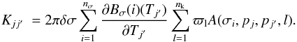${\mathit{K}}_{\mathit{j}{\mathit{j}}^{\mathrm{\prime }}}\mathrm{=}\mathrm{2}\mathit{\pi \delta \sigma }\sum _{\mathit{i}\mathrm{=}\mathrm{1}}^{{\mathit{n}}_{\mathit{\sigma }}}\frac{\mathit{\partial }{\mathit{B}}_{\mathit{\sigma }}\mathrm{\left(}\mathit{i}\mathrm{\right)}\mathrm{\left(}{\mathit{T}}_{{\mathit{j}}^{\mathrm{\prime }}}\mathrm{\right)}}{\mathit{\partial }{\mathit{T}}_{{\mathit{j}}^{\mathrm{\prime }}}}\sum _{\mathit{l}\mathrm{=}\mathrm{1}}^{{\mathit{n}}_{\mathrm{k}}}{\mathit{\varpi }}_{\mathrm{l}}\mathit{A}\mathrm{\left(}{\mathit{\sigma }}_{\mathit{i}}\mathit{,}{\mathit{p}}_{\mathit{j}}\mathit{,}{\mathit{p}}_{{\mathit{j}}^{\mathrm{\prime }}}\mathit{,l}\mathrm{\right)}\mathit{.}$(A.7)Matrix C is equal to ${C}\mathrm{=}\mathit{\alpha }{{KSK}}^{\mathit{T}}\mathrm{+}{E}\mathit{,}$(A.8)where E is a diagonal matrix with E_jj′ equal to the square of the flux error acceptable at the jth pressure level, usually set to 0.1% of $\mathit{\sigma }{\mathit{T}}_{\mathrm{eff}}^{\mathrm{4}}$.

The nonlinearity of the problem requires an iterative process in which T_n is obtained from Eq. (A.6) after updating the reference profile to T_{n − 1} and recalculating the kernel matrix K for profile T_{n − 1}. The iteration process is pursued until χ² is less than 1 and no longer significantly decreases. The α parameter in Eq. (A.7) is chosen to be small enough to ensure convergence and large enough to reduce the number of iterations needed. Typically ten iterations are needed. Note that the final solution does not depend on the initial profile T₀ or on the choice of α. For T₀, we used one of the three temperature profiles calculated by Allard et al. (2003) for T_eff = 900, 1300, and 1700 K. We choose that having T_eff closest to the input value to ensure rapid convergence.

In a second step, the solution profile is checked against convective instability by comparing the model lapse rate $\mathrm{▽}\mathrm{=}\frac{\ln \mathrm{(}{\mathit{T}}_{\mathit{j}}\mathit{/}{\mathit{T}}_{\mathit{j}\mathrm{-}\mathrm{1}}\mathrm{)}}{\ln \mathrm{(}{\mathit{p}}_{\mathit{j}}\mathit{/}{\mathit{p}}_{\mathit{j}\mathrm{-}\mathrm{1}}\mathrm{)}}$ with the adiabatic value ▽ _ad = R/C_p, where R is the gas constant and C_p the temperature-dependent molar heat capacity for the H₂-He atmosphere. Regions where the lapse rate exceeds the adiabatic value are unstable against convection. They are found in the bottom of the pressure grid p>p_ad, with p_ad being the level where the lapse rate equals the adiabatic value. In that case, convective heat transfer occurs setting back the lapse rate to the adiabatic value. In Exo-REM, we do not solve explicitly for convection. We add a convective flux to the radiative flux in Eq. (A.4) through an analytical function that is essentially zero when ▽ ≤ ▽ _ad and rapidly gets very large when ▽ > ▽ _ad. We found that the following function: ${\mathit{F}}_{\mathrm{conv}}\mathrm{\left(}{\mathit{p}}_{\mathit{j}}\mathrm{\right)}\mathrm{=}{\mathrm{10}}^{-3}\mathit{\sigma }{\mathit{T}}_{\mathrm{eff}}^{\mathrm{4}}{\mathrm{e}}^{\mathrm{200}\mathrm{[}\mathrm{▽}\mathit{/}{\mathrm{▽}}_{\mathrm{ad}}\mathrm{-}\mathrm{1}\mathrm{]}}$(A.9)is adequate to ensure negligible superadiabaticity in the final solution profile. We then set the lapse rate of the purely radiative solution to the adiabatic value, plus a small amount (0.015), at levels p>p_ad . The kernel matrix K is calculated adding $\begin{array}{ccc}\frac{\mathit{\partial }{\mathit{F}}_{\mathrm{conv}}\mathrm{\left(}{\mathit{p}}_{\mathit{j}}\mathrm{\right)}}{\mathit{\partial }{\mathit{T}}_{\mathit{j}}}& \mathrm{=}& \mathrm{0.2}\mathit{\sigma }{\mathit{T}}_{\mathrm{eff}}^{\mathrm{4}}{\mathrm{e}}^{\mathrm{200}\mathrm{[}\mathrm{▽}\mathit{/}{\mathrm{▽}}_{\mathrm{ad}}\mathrm{-}\mathrm{1}\mathrm{]}}\mathit{/}\mathrm{\left(}{\mathit{T}}_{\mathit{j}}{\mathrm{▽}}_{\mathrm{ad}}\ln \mathrm{\right(}{\mathit{p}}_{\mathit{j}}\mathit{/}{\mathit{p}}_{\mathit{j}\mathrm{-}\mathrm{1}}\mathrm{\left)}\mathrm{\right)}\mathrm{\left(}\mathit{a}\mathrm{\right)}\\ \mathrm{to}{\mathit{K}}_{\mathit{jj}}\mathrm{and}& & \\ \frac{\mathit{\partial }{\mathit{F}}_{\mathrm{conv}}\mathrm{\left(}{\mathit{p}}_{\mathit{j}}\mathrm{\right)}}{\mathit{\partial }{\mathit{T}}_{\mathit{j}\mathrm{-}\mathrm{1}}}& \mathrm{=}& \mathrm{-}\mathrm{0.2}\mathit{\sigma }{\mathit{T}}_{\mathrm{eff}}^{\mathrm{4}}{\mathrm{e}}^{\mathrm{200}\mathrm{[}\mathrm{▽}\mathit{/}{\mathrm{▽}}_{\mathrm{ad}}\mathrm{-}\mathrm{1}\mathrm{]}}\mathit{/}\mathrm{\left(}{\mathit{T}}_{\mathit{j}\mathrm{-}\mathrm{1}}{\mathrm{▽}}_{\mathrm{ad}}\ln \mathrm{\right(}{\mathit{p}}_{\mathit{j}}\mathit{/}{\mathit{p}}_{\mathit{j}\mathrm{-}\mathrm{1}}\mathrm{\left)}\mathrm{\right)}\mathrm{\left(}\mathit{b}\mathrm{\right)}\mathit{,}\end{array}$(A.10)to K_{jj − 1} in Eq. (A.7). The iterative process is finally restarted with the modified flux and kernel until convergence is achieved. Typically another set of ten iterations is needed. Our model in this paper has 64 pressure levels equally spaced in ln(p) between 50 bar and 0.01 mbar.

All Tables

All Figures

References

- Ackerman, A. S., & Marley, M. S. 2001, ApJ, 556, 872 [NASA ADS] [CrossRef] [Google Scholar]
- Albert, S., Bauerecker, S., Boudon, V., et al. 2009, Chem. Phys., 356, 131 [NASA ADS] [CrossRef] [Google Scholar]
- Allard, F., Hauschildt, P. H., Alexander, D. R., Tamanai, A., & Schweitzer, A. 2001, ApJ, 556, 357 [NASA ADS] [CrossRef] [Google Scholar]
- Allard, F., Guillot, T., Ludwig, H.-G., et al. 2003, in Brown Dwarfs, ed. E. Martín, IAU Symp., 211, 325 [Google Scholar]
- Allard, F., Allard, N. F., Homeier, D., et al. 2007, A&A, 474, L21 [NASA ADS] [CrossRef] [EDP Sciences] [Google Scholar]
- Barman, T. S., Macintosh, B., Konopacky, Q. M., & Marois, C. 2011, ApJ, 733, 65 [NASA ADS] [CrossRef] [Google Scholar]
- Barman, T. S., Konopacky, Q. M., Macintosh, B., & Marois, C. 2015, ApJ, 804, 61 [NASA ADS] [CrossRef] [Google Scholar]
- Baudino, J.-L., Bézard, B., Boccaletti, A., Lagrange, A., & Bonnefoy, M. 2013, BAAS, 45, 209.09 [Google Scholar]
- Baudino, J.-L., Bézard, B., Boccaletti, A., Bonnefoy, M., & Lagrange, A.-M. 2014a, in Exploring the Formation and Evolution of Planetary Systems, eds. M. Booth, B. C. Matthews, & J. R. Graham, Proc. IAU Symp., 299, 277 [Google Scholar]
- Baudino, J.-L., Bézard, B., Boccaletti, A., et al. 2014b, in SF2A Proceedings, eds. J. Ballet, F. Martins, F. Bournaud, R. Monier, & C. Reylé, 53 [Google Scholar]
- Beuzit, J.-L., Feldt, M., Dohlen, K., et al. 2008, Proc. SPIE, 7014, 18 [Google Scholar]
- Bevington, P. R., & Robinson, D. K. 2003, Data reduction and error analysis for the physical sciences (McGraw-Hill) [Google Scholar]
- Binks, A. S., & Jeffries, R. D. 2014, MNRAS, 438, L11 [NASA ADS] [CrossRef] [Google Scholar]
- Boccaletti, A., Baudoz, P., Baudrand, J., Reess, J. M., & Rouan, D. 2005, Adv. Space Res., 36, 1099 [Google Scholar]
- Bonnefoy, M., Lagrange, A.-M., Boccaletti, A., et al. 2011, A&A, 528, L15 [NASA ADS] [CrossRef] [EDP Sciences] [Google Scholar]
- Bonnefoy, M., Boccaletti, A., Lagrange, A.-M., et al. 2013, A&A, 555, A107 [NASA ADS] [CrossRef] [EDP Sciences] [Google Scholar]
- Bonnefoy, M., Marleau, G.-D., Galicher, R., et al. 2014, A&A, 567, L9 [NASA ADS] [CrossRef] [EDP Sciences] [Google Scholar]
- Borysow, A. 2002, A&A, 390, 779 [NASA ADS] [CrossRef] [EDP Sciences] [Google Scholar]
- Borysow, A., & Frommhold, L. 1989, ApJ, 341, 549 [NASA ADS] [CrossRef] [Google Scholar]
- Borysow, J., Frommhold, L., & Birnbaum, G. 1988, ApJ, 326, 509 [NASA ADS] [CrossRef] [Google Scholar]
- Borysow, A., Frommhold, L., & Moraldi, M. 1989, ApJ, 336, 495 [NASA ADS] [CrossRef] [Google Scholar]
- Borysow, U., Jorgensen, A., & Fu, Y. 2001, J. Quant. Spec. Radiat. Transf., 68, 235 [NASA ADS] [CrossRef] [Google Scholar]
- Boss, A. P. 2001, ApJ, 551, L167 [NASA ADS] [CrossRef] [Google Scholar]
- Boudon, V., Rey, M., & Loëte, M. 2006, J. Quant. Spec. Radiat. Transf., 98, 394 [NASA ADS] [CrossRef] [Google Scholar]
- Bowler, B. P., Liu, M. C., Dupuy, T. J., & Cushing, M. C. 2010, ApJ, 723, 850 [NASA ADS] [CrossRef] [Google Scholar]
- Burrows, A., & Sharp, C. M. 1999, ApJ, 512, 843 [NASA ADS] [CrossRef] [Google Scholar]
- Burrows, A., & Volobuyev, M. 2003, ApJ, 583, 985 [NASA ADS] [CrossRef] [Google Scholar]
- Burrows, A., Saumon, D., Guillot, T., Hubbard, W. B., & Lunine, J. I. 1995, Nature, 375, 299 [NASA ADS] [CrossRef] [Google Scholar]
- Burrows, A., Marley, M. S., & Sharp, C. M. 2000, ApJ, 531, 438 [NASA ADS] [CrossRef] [Google Scholar]
- Burrows, A., Sudarsky, D., & Hubeny, I. 2006, ApJ, 640, 1063 [NASA ADS] [CrossRef] [Google Scholar]
- Campargue, A., Wang, L., Mondelain, D., et al. 2012, Icarus, 219, 110 [NASA ADS] [CrossRef] [Google Scholar]
- Chabrier, G., Baraffe, I., Allard, F., & Hauschildt, P. 2000, ApJ, 542, 464 [NASA ADS] [CrossRef] [Google Scholar]
- Chase, Jr., M. W. 1998, NIST-JANAF Thermochemical Tables, 4th edn., Monograph No. 9 [Google Scholar]
- Chauvin, G., Lagrange, A.-M., Dumas, C., et al. 2004, A&A, 425, L29 [NASA ADS] [CrossRef] [EDP Sciences] [MathSciNet] [Google Scholar]
- Chilcote, J., Barman, T., Fitzgerald, M. P., et al. 2015, ApJ, 798, L3 [NASA ADS] [CrossRef] [Google Scholar]
- Claudi, R. U., Turatto, M., Gratton, R. G., et al. 2008, Proc. SPIE, 7014, 3 [Google Scholar]
- Close, L. M., Males, J. R., Kopon, D. A., et al. 2012, Proc. SPIE, 8447, 16 [Google Scholar]
- Conrath, B. J., Gierasch, P. J., & Ustinov, E. A. 1998, Icarus, 135, 501 [NASA ADS] [CrossRef] [Google Scholar]
- Currie, T., Burrows, A., Madhusudhan, N., et al. 2013, ApJ, 776, 15 [NASA ADS] [CrossRef] [Google Scholar]
- Daumont, L., Nikitin, A. V., Thomas, X., et al. 2013, J. Quant. Spectr. Rad. Transf., 116, 101 [NASA ADS] [CrossRef] [Google Scholar]
- Galicher, R., Rameau, J., Bonnefoy, M., et al. 2014, A&A, 565, L4 [NASA ADS] [CrossRef] [EDP Sciences] [Google Scholar]
- Goody, R. M., & Yung, Y. L. 1989, Atmospheric radiation: theoretical basis (Oxford University Press) [Google Scholar]
- Hanot, C., Absil, O., Surdej, J., Boccaletti, A., & Vérinaud, C. 2010, Proc. SPIE, 7731, 3 [Google Scholar]
- Hartmann, J.-M., Boulet, C., Brodbeck, C., et al. 2002, J. Quant. Spectr. Rad. Transf., 72, 117 [NASA ADS] [CrossRef] [Google Scholar]
- Helling, C., Ackerman, A., Allard, F., et al. 2008, MNRAS, 391, 1854 [NASA ADS] [CrossRef] [Google Scholar]
- Jäger, C., Dorschner, J., Mutschke, H., Posch, T., & Henning, T. 2003, A&A, 408, 193 [NASA ADS] [CrossRef] [EDP Sciences] [Google Scholar]
- Janson, M., Bergfors, C., Goto, M., Brandner, W., & Lafrenière, D. 2010, ApJ, 710, L35 [NASA ADS] [CrossRef] [Google Scholar]
- Konopacky, Q. M., Barman, T. S., Macintosh, B. A., & Marois, C. 2013, Science, 339, 1398 [NASA ADS] [CrossRef] [Google Scholar]
- Kramida, A., Yu. Ralchenko, Reader, J., & NIST ASD Team. 2014, NIST Atomic Spectra Database, ver. 5.2, [Online], available: http://physics.nist.gov/asd [2015, March 17], National Institute of Standards and Technology, Gaithersburg, MD [Google Scholar]
- Lagrange, A.-M., Gratadour, D., Chauvin, G., et al. 2009, A&A, 493, L21 [NASA ADS] [CrossRef] [EDP Sciences] [Google Scholar]
- Lagrange, A.-M., Bonnefoy, M., Chauvin, G., et al. 2010, Science, 329, 57 [NASA ADS] [CrossRef] [PubMed] [Google Scholar]
- Lagrange, A.-M., Boccaletti, A., Milli, J., et al. 2012a, A&A, 542, A40 [NASA ADS] [CrossRef] [EDP Sciences] [Google Scholar]
- Lagrange, A.-M., De Bondt, K., Meunier, N., et al. 2012b, A&A, 542, A18 [NASA ADS] [CrossRef] [EDP Sciences] [Google Scholar]
- Lagrange, A.-M., Meunier, N., Chauvin, G., et al. 2013, A&A, 559, A83 [NASA ADS] [CrossRef] [EDP Sciences] [Google Scholar]
- Lagrange, A.-M., Gilardy, H., Beust, H., et al. 2014, in Exploring the Formation and Evolution of Planetary Systems, eds. M. Booth, B. C. Matthews, & J. R. Graham, Proc. IAU Symp., 299, 299 [Google Scholar]
- Langlois, M., Dohlen, K., Augereau, J.-C., et al. 2010, Proc. SPIE, 7735, 2 [Google Scholar]
- Lecavelier Des Etangs, A., Vidal-Madjar, A., Burki, G., et al. 1997, A&A, 328, 311 [NASA ADS] [Google Scholar]
- Lenzen, R., Hartung, M., Brandner, W., et al. 2003, in Instrument Design and Performance for Optical/Infrared Ground-based Telescopes, eds. M. Iye, & A. F. M. Moorwood, Proc. SPIE, 4841, 944 [Google Scholar]
- Lin, D. N. C., & Ida, S. 1997, ApJ, 477, 781 [NASA ADS] [CrossRef] [Google Scholar]
- Lodders, K. 2010, in Principles and Perspectives in Cosmochemistry, eds. A. Goswami, & B. E. Reddy (Berlin: Springer), 379 [Google Scholar]
- Lodders, K., & Fegley, Jr., B. 2006, Chemistry of Low Mass Substellar Objects, ed. J. W. Mason, 1 [Google Scholar]
- Lunine, J. I., Hubbard, W. B., Burrows, A., Wang, Y.-P., & Garlow, K. 1989, ApJ, 338, 314 [NASA ADS] [CrossRef] [Google Scholar]
- Macintosh, B., Graham, J. R., Ingraham, P., et al. 2014, Proc. of the National Academy of Science, 111, 12661 [Google Scholar]
- Males, J. R., Close, L. M., Morzinski, K. M., et al. 2014, ApJ, 786, 32 [NASA ADS] [CrossRef] [Google Scholar]
- Marleau, G.-D., & Cumming, A. 2014, MNRAS, 437, 1378 [NASA ADS] [CrossRef] [Google Scholar]
- Marley, M., Ackerman, A., & Seager, S. 2000, BAAS, 32, 127.05 [Google Scholar]
- Marley, M. S., Saumon, D., Cushing, M., et al. 2012, ApJ, 754, 135 [NASA ADS] [CrossRef] [Google Scholar]
- Marois, C., Macintosh, B., Barman, T., et al. 2008, Science, 322, 1348 [NASA ADS] [CrossRef] [PubMed] [Google Scholar]
- Mayor, M., & Queloz, D. 1995, Nature, 378, 355 [NASA ADS] [CrossRef] [Google Scholar]
- Mordasini, C., Alibert, Y., Georgy, C., et al. 2012, A&A, 547, A112 [NASA ADS] [CrossRef] [EDP Sciences] [Google Scholar]
- Morley, C. V., Fortney, J. J., Marley, M. S., et al. 2012, ApJ, 756, 172 [NASA ADS] [CrossRef] [Google Scholar]
- Mouillet, D., Larwood, J. D., Papaloizou, J. C. B., & Lagrange, A. M. 1997, MNRAS, 292, 896 [NASA ADS] [CrossRef] [PubMed] [Google Scholar]
- Neuhäuser, R., Guenther, E. W., Wuchterl, G., et al. 2005, A&A, 435, L13 [NASA ADS] [CrossRef] [EDP Sciences] [Google Scholar]
- Nikitin, A., Brown, L. R., Féjard, L., Champion, J. P., & Tyuterev, V. G. 2002, J. Mol. Spectr., 216, 225 [NASA ADS] [CrossRef] [Google Scholar]
- Nikitin, A. V., Champion, J.-P., & Brown, L. R. 2006, J. Mol. Spectr., 240, 14 [NASA ADS] [CrossRef] [Google Scholar]
- Nikitin, A. V., Brown, L. R., Sung, K., et al. 2013, J. Quant. Spec. Radiat. Transf., 114, 1 [NASA ADS] [CrossRef] [Google Scholar]
- Ordal, M. A., Bell, R. J., Alexander, Jr., R. W., Newquist, L. A., & Querry, M. R. 1988, Appl. Opt., 27, 1203 [NASA ADS] [CrossRef] [PubMed] [Google Scholar]
- Plez, B. 1998, A&A, 337, 495 [NASA ADS] [Google Scholar]
- Quanz, S. P., Meyer, M. R., Kenworthy, M. A., et al. 2010, ApJ, 722, L49 [NASA ADS] [CrossRef] [Google Scholar]
- Rameau, J., Chauvin, G., Lagrange, A.-M., et al. 2013, ApJ, 772, L15 [NASA ADS] [CrossRef] [Google Scholar]
- Rothman, L. S., Gordon, I. E., Barber, R. J., et al. 2010, J. Quant. Spectr. Rad. Transf., 111, 2139 [NASA ADS] [CrossRef] [Google Scholar]
- Rousset, G., Lacombe, F., Puget, P., et al. 2003, in Adaptive Optical System Technologies II, eds. P. L. Wizinowich, & D. Bonaccini, Proc. SPIE, 4839, 140 [Google Scholar]
- Rowe, J. F., Coughlin, J. L., Antoci, V., et al. 2015, ApJS, 217, 16 [NASA ADS] [CrossRef] [Google Scholar]
- Schmid, H. M., Beuzit, J. L., Mouillet, D., et al. 2010, in Proc. Conf. In the Spirit of Lyot 2010, 49 [Google Scholar]
- Smith, B. A., & Terrile, R. J. 1987, BAAS, 19, 829 [NASA ADS] [Google Scholar]
- Spiegel, D. S., & Burrows, A. 2012, ApJ, 745, 174 [NASA ADS] [CrossRef] [Google Scholar]
- Tsuji, T. 2002, ApJ, 575, 264 [NASA ADS] [CrossRef] [Google Scholar]
- Tsuji, T., Ohnaka, K., & Aoki, W. 1996, A&A, 305, L1 [NASA ADS] [Google Scholar]
- van Leeuwen, F. 2007, A&A, 474, 653 [NASA ADS] [CrossRef] [EDP Sciences] [Google Scholar]
- Vigan, A., Moutou, C., Langlois, M., et al. 2010, MNRAS, 407, 71 [NASA ADS] [CrossRef] [Google Scholar]
- Vinatier, S., Bézard, B., Fouchet, T., et al. 2007, Icarus, 188, 120 [NASA ADS] [CrossRef] [Google Scholar]
- Yurchenko, S. N., & Tennyson, J. 2014, MNRAS, 440, 1649 [NASA ADS] [CrossRef] [Google Scholar]
- Yurchenko, S. N., Barber, R. J., & Tennyson, J. 2011, MNRAS, 413, 1828 [NASA ADS] [CrossRef] [Google Scholar]