| Issue |
A&A
Volume 582, October 2015
|
|
|---|---|---|
| Article Number | A64 | |
| Number of page(s) | 17 | |
| Section | Interstellar and circumstellar matter | |
| DOI | https://doi.org/10.1051/0004-6361/201526220 | |
| Published online | 08 October 2015 | |
Tentative detection of ethylene glycol toward W51/e2 and G34.3+0.2 ⋆,⋆⋆,⋆⋆⋆
1
Centre for Star and Planet Formation, Niels Bohr Institute &
Natural History Museum of Denmark, University of Copenhagen,
Øster Voldgade 5–7,
1350
Copenhagen K.,
Denmark
e-mail:
This email address is being protected from spambots. You need JavaScript enabled to view it.
2
Department of Astronomy, University of Michigan,
500 Church Street, Ann Arbor, MI
48109,
USA
Received: 30 March 2015
Accepted: 4 July 2015
Abstract
Context. With only a few low- and high-mass star-formation regions studied in detail so far, it is unclear what role the enviroment plays in complex molecule formation. In this light, a comparison of relative abundances of related species between sources might be useful for explaining any observed differences.
Aims. We seek to measure the relative abundance between three important complex organic molecules, ethylene glycol ((CH2OH)2), glycolaldehyde (CH2OHCHO) and methyl formate (HCOOCH3), toward high-mass protostars and thereby provide additional constraints on their formation pathways.
Methods. We use IRAM 30 m single-dish observations of the three species toward two high-mass star-forming regions – W51/e2 and G34.3+0.2 – and report a tentative detection of (CH2OH)2 toward both sources.
Results. Assuming that (CH2OH)2, CH2OHCHO, and HCOOCH3 spatially coexist, relative abundance ratios, HCOOCH3/(CH2OH)2, of 31 and 35 are derived for G34.3+0.2 and W51/e2, respectively. CH2OHCHO is not detected, but the data provide lower limits to the HCOOCH3/CH2OHCHO abundance ratios of ≥193 for G34.3+0.2 and ≥550 for W51/e2. A comparison of these results to measurements from various sources in the literature indicates that the source luminosities may be correlated with the HCOOCH3/(CH2OH)2 and HCOOCH3/CH2OHCHO ratios. This apparent correlation may be a consequence of the relative time scales each source spend at different temperature ranges in their evolution. Furthermore, we obtain lower limits to the ratio of (CH2OH)2/CH2OHCHO for G34.3+0.2 (≥6) and W51/e2 (≥16). This result confirms that a high (CH2OH)2/CH2OHCHO abundance ratio is not a specific property of comets, as previously speculated.
Key words: ISM: molecules / ISM: abundances / ISM: individual objects: W51/e2 / methods: observational / astrochemistry / ISM: individual objects: G34.3+0.2
Based on observations carried out with the IRAM 30 m telescope.
The reduced spectra (FITS files) are only available at the CDS via anonymous ftp to cdsarc.u-strasbg.fr (130.79.128.5) or via http://cdsarc.u-strasbg.fr/viz-bin/qcat?J/A+A/582/A64
Appendices are available in electronic form at http://www.aanda.org
© ESO, 2015
1. Introduction
How complex organic – and potentially prebiotic – molecules are formed in regions of low- and high-mass star formation remains a central question in astrochemistry. To date there has been no consensus about how complex organic molecules (COMs hereafter) form in dense regions of the interstellar medium, despite the increasing number of detections (e.g., Herbst & van Dishoeck 2009). One promising suggestion was that warm gas phase chemistry, following evaporation of simple ices, could be a primary formation pathway (e.g., Millar et al. 1991; Charnley et al. 1992). However, more recent laboratory experiments and chemical modeling has shown that this mechanism is not effective enough to account for the observed abundances (e.g., Geppert et al. 2006). An alternative formation mechanism involves UV induced radicals. Garrod et al. (2008) propose that, during the warm up phase, radicals can migrate on the grains surfaces and form complex species that are then released into the gas phase at higher temperatures. The initial ice composition and the amount of UV radiation have also proved to play an important part in the formation process (Öberg et al. 2009). To determine the formation pathway of COMs, it is useful to determine abundance ratios between different related species because these ratios, in comparison with the predicted abundance ratios from chemical models, can provide constraints on the formation processes. Indeed, variations in the abundance profiles can reflect the physical and chemical conditions that are occurring. It is therefore important to observe these species in different environments.
Some of the simplest species in this context include the oxygen-bearing COMs associated to glycolaldehyde, CH2OHCHO, including its isomer methyl formate (HCOOCH3 or CH3OCHO) and the reduced alcohol version of CH2OHCHO, ethylene glycol, (CH2OH)2 (also commonly known as anti-freeze). By constraining the relative abundances of these species in different environments the hope is to be able to explore, for instance, the importance of initial chemical conditions, temperature and irradiation in the formation for comparison, such as for laboratory experiments (e.g., Öberg et al. 2009) and as input for sophisticated chemical models (e.g., Garrod et al. 2008). For example, in their laboratory experiments Öberg et al. (2009) show that the relative abundances of HCOOCH3 to CH2OHCHO and (CH2OH)2 strongly depend on both the ice temperature and exact ice composition in terms of the relative amounts of CO and CH3OH.
So far, (CH2OH)2 has been detected toward high-mass sources such as the Galactic center source Sgr B2(N) by Hollis et al. (2002), marginally toward W51 e1/e2 by Kalenskii & Johansson (2010), and recently also toward the Orion Kleinmann-Low (KL) nebula by Brouillet et al. (2015). (CH2OH)2 has also been observed toward the low-mass Class 0 protostars IRAS 16293–2422 (Jørgensen et al. 2012, and in prep.) and NGC 1333 IRAS 2A (Maury et al. 2014; Coutens et al. 2015) as well as toward the intermediate-mass protostar NGC 7129 FIRS2 (Fuente et al. 2014). CH2OHCHO has been detected toward Sgr B2(N) (Hollis et al. 2000, 2001, 2004; Halfen et al. 2006; Requena-Torres et al. 2008), the high-mass hot molecular core G31.41+0.31 (Beltrán et al. 2009), in IRAS 16293–2422 by Jørgensen et al. (2012) and recently also in NGC 7129 FIRS2 (Fuente et al. 2014), NGC 1333 IRAS 2A (Coutens et al. 2015; Taquet et al. 2015) and NGC 1333 IRAS 4A (Taquet et al. 2015). HCOOCH3 is the most abundant isomer of CH2OHCHO, and it has previously been observed in numerous hot cores and corinos (e.g., Blake et al. 1987; Bisschop et al. 2007; Demyk et al. 2008; Favre et al. 2014, 2011). There are some notable differences in terms of the abundance ratios. For example, Coutens et al. (2015) find a (CH2OH)2/CH2OHCHO ratio of ~5 in NGC 1333 IRAS 2A, while Jørgensen et al. (2012 and in prep.) find a lower value of ~1 in IRAS 16293-2422. These changes hint that it might be useful to explore these ratios in different sources sampling similar physical conditions.
This paper presents IRAM 30 m observations of (CH2OH)2 and CH2OHCHO toward the high-mass protostars W51/e2 (distance = 5.4 kpc, Sato et al. 2010) and G34.3+0.2 (distance = 3.8 kpc, Kurtz et al. 2000). The aim of this study is to determine the relative abundance of (CH2OH)2 and CH2OHCHO to HCOOCH3 and compare to other sources from the literature. Overall our aim is to investigate the use of abundance ratios of species that are believed to be chemically related to explore the origin of complex molecules in the dense interstellar medium. In Sect. 2, the IRAM 30 m observations are presented. Data modeling, results and analysis are presented in Sect. 3 and discussed in Sect. 4.
2. Observations
Transitions of (CH2OH)2 in the observed frequency range.
The observations were performed with the IRAM 30 m telescope at Pico Veleta, Spain on December 13 and 14, 2012 for W51/e2 and G34.3+0.2, respectively. The coordinates of the phase tracking center used for the two sources were αJ2000 = 19h23m43 9, δJ2000 = 14°30′34
 8 for W51/e2 and αJ2000 = 18h53m186, δJ2000 = 01°14′580 for G34.3+0.2. The observations were performed in position-switching mode using [−600″,0″ ] as reference for the OFF positions. The spectral setup was chosen to target (CH2OH)2 and CH2OHCHO in the observations. The EMIR receiver was used in dual-band polarisation (E090/E230) in connection with i) the 200 kHz Fourier transform spectrometer (FTS) backend in the frequency ranges 99.70–106.3 GHz and 238.2–246.0 GHz for the E090 and E230 bands, respectively; ii) the WILMA backend in the frequency ranges 99.88–103.6 GHz and 238.4–242.1 GHz for the E090 and E230 bands, respectively. Data was reduced with the Continuum and Line Analysis Single-dish Software1 (CLASS). The resulting FTS spectra were smoothed to a spectral resolution of 1.15 km s-1 for the E090 band and 1.22 km s-1 for the E230 band, while the WILMA spectra were smoothed to 5.88 km s-1 and 2.49 km s-1 for the E090 and E230 bands, respectively. Spectra resulting from the FTS backend presented a standing wave pattern, and the WILMA observations were therefore used as a sanity check for the FTS data and for confirmation of the detections made in the FTS observations for the lines where the frequency of the two sets of observations match. The standing wave present in the FTS observations was removed using a fast Fourier transform in the data reduction.
Throughout this paper, the intensity is given as the main beam brightness temperature (Tmb), which is defined as  where Ta is the antenna temperature, Feff the forward efficiency and Beff the beam efficiency. The values used were Feff = 0.94 and 0.92 and Beff = 0.78 and 0.58 for 1 mm and 3 mm respectively. The half-power beam sizes are ~10″ and ~24″ for the observations at 1 mm and 3 mm, respectively.
3. Analysis and results
 |
Fig. 1 Observed (black) and synthetic (red) spectra of the five transitions of (CH2OH)2 in W51/e2 that are used for the analysis. Also shown are the synthetic spectra of all other species investigated in this study (blue) to demonstrate that the (CH2OH)2 lines in question are not blended. The transitions are located at 239 883.56, 240 807.88, 242 656.23, 242 948.29 and 100 333.64 MHz – denoted by black vertical lines in the plot. The displayed frequency region in each plot corresponds to ~200 km s-1. |
 |
Fig. 2 Same as for Fig. 1 but for G34.3+0.2. The transitions are located at 240 807.88 and 242 656.23 MHz – indicated by black vertical lines in the plot. |
Spectra from both sources show a rich forest of lines characteristic of high-mass sources. A total of 21 and 19 lines have peak temperatures above 5 K for W51/e2 and G34.3+0.2, respectively. The strongest lines in both spectra are the CS 5–4 transition at 244 935 MHz. It is important to know that there is still a remnant oscillation in the baseline even after the removal of the standing wave in the spectra. This increases the rms noise of the spectra, which complicates the analysis of faint lines. Therefore, in addition to the global baseline subtraction, an additional local zero-, or first-order baseline subtraction was therefore performed before making a Gaussian fit of the (CH2OH)2 lines. This additional baseline subtraction is applied in a range of ±100 km s-1 for each line. As for the data reduction, CLASS was used for the additional baseline subtraction, as well as for Gaussian profile fits to the detected lines. The resulting rms of the local baseline is ~60 mK for the 1 mm observations and ~7 mK for the 3 mm observations.
To ensure proper line identification, we checked the line observations against entries in the Splatalogue database for astronomical spectroscopy2. In addition, we made a reference model where we produced synthetic spectra for the line emission of common species (CH3OCH3, HCOOH, CH3CHO, CH3OH, C2H5OH and CH3CN) in order to visually exclude lines that are blended with any of these molecules. Table 1 lists spectroscopic parameters for the (CH2OH)2 transitions that can be excited in the observed frequency range. Transitions with log (Aul) < −5 for the 3 mm observations and log (Aul) < −4 and Eup> 300 K for the 1 mm observations have been excluded from the table, because these transitions are predicted from the synthetic spectra to have peak intensities ≲0.02 K, i.e., are not detectable.
The spectroscopic data for (CH2OH)2 come from Christen & Müller (2003) and Christen et al. (1995) and are available from the CDMS database3 (Müller et al. 2001, 2005), while the spectroscopic data for HCOOCH3 and CH2OHCHO are from Ilyushin et al. (2009) and Carroll et al. (2010) respectively, available from the JPL database4 (Pickett et al. 1998). For the analysis, the (CH2OH)2 lines that are reasonably well separated and have a peak temperature above 3σ were selected. For W51/e2 we included the lines at ~100 333 and ~242 656 MHz, although they are partially blended, because it is possible to distinguish the (CH2OH)2 peak from the other peaks and perform a multiple Gaussian fit that includes all relevant peaks.
Transitions of (CH2OH)2 observed toward W51/e2 and G34.3+0.2 with the IRAM 30–m telescope.
Figures 1 and 2 show a zoom-in of the area of ~200 km s-1, which corresponds to ~160 MHz in the 1 mm observations and ~70 MHz in the 3 mm observations, around each detected line in both sources after the local baseline subtraction. Superimposed onto the observed spectra are the synthetic spectra of (CH2OH)2 as well as the other species investigated here, as to demonstrate that the chosen (CH2OH)2 lines are not blended. The fit to the entire observed spectra for both sources are shown in Figs. B.1–B.8 in the appendix. Table A.1 in the appendix lists the estimated column densities of the molecules in the reference model. Table 2 lists spectroscopic parameters and the observed quantities from the fits of the (CH2OH)2 lines: the integrated line intensity ( ), position (VLSR), line width (Δv) and peak temperature (Peak Tmb).
A total of 35 and 52 well separated lines have been detected above the 3σ level in the 1 mm and 3 mm data for HCOOCH3 in W51/e2 and G34.3+0.2, respectively. For (CH2OH)2, four and two lines toward W51/e2 and G34.3+0.2 respectively, are detected in the 1 mm observations; while only one line is detected at 3 mm toward W51/e2. Many other (CH2OH)2 lines, as well as some potential CH2OHCHO lines are present in both data sets, but they are either blended with other species or too faint to be properly detected above a 3σ limit.
3.1. Modeling
Assuming LTE and optically thin emission, the rotational diagram method can be used to determine the column density, Ntot, and the rotational temperature, Trot (Goldsmith & Langer 1999). The approach used in this work follows the formalism described by Goldsmith & Langer (1999) with the following assumptions:
-
1.
(CH2OH)2, CH2OHCHO, and HCOOCH3 are emitting from the same region and thus have the same source size, θsource.
-
2.
(CH2OH)2, CH2OHCHO, and HCOOCH3 are in LTE, which implies that the excitation temperature, Tex, is equal to the kinematic temperature, Tkin, for all three species. Using the rotational diagram method, one obtains the rotational temperature, which in LTE is Tkin = Trot = Tex.
-
3.
The observations at 1 mm and 3 mm trace the same gas.
According to our assumptions, the source size and Trot derived from the HCOOCH3 analysis can be used to derive the column density of (CH2OH)2 and set an upper limit on the column density of CH2OHCHO. A possible caveat is that the large beam size of our observations compared to the source sizes does not guarantee that the measured lines arise from species present in the same gas. Specifically, we obtain similar mean values of VLSR for (CH2OH)2 and HCOOCH3 in both sources (56.4 ± 0.5 km s-1 and 56.0 ± 0.8 km s-1 in W51/e2 along with 57.7 ± 0.5 km s-1 and 58.4 ± 1.2 km s-1 in G34.3+0.2 for (CH2OH)2 and HCOOCH3, respectively), so here the assumption appears reasonable.
The same formalism in Goldsmith & Langer (1999) as was used to create a rotational diagram can also be used to generate a synthetic spectrum of the line emission of a specific molecule by using the source size, θsource, the rotational temperature, Trot, the line width, Δv, and the column density, Ntot, as input parameters. It is possible to correct for the optical depth of the line emission in case it deviates from being completely optically thin (Goldsmith & Langer 1999). A synthetic spectrum generated with input parameters derived from the rotational diagram therefore serves as a check for the self-consistency of the result. We use adopted source sizes from the literature and determine the rotational temperatures and column densities in the following analysis.
The observed width of the detected lines have been determined from the Gaussian fit. For HCOOCH3 in W51/e2, we obtain mean values of Δv = 6.4 ± 0.8 km s-1 in the 1 mm data and Δv = 6.1 ± 1.1 km s-1 in the 3 mm data. In the same source, the mean value of the line width of the (CH2OH)2 lines is 6.3 ± 0.9 km s-1 for the 1 mm data, and the only detected value is 5.5 km s-1 in the 3 mm data. For G34.3+0.2, we find Δv = 6.5 ± 1.5 km s-1 in the 1 mm data and Δv = 7.3 ± 1.3 km s-1 in the 3 mm data for HCOOCH3 and Δv = 4.5 ± 0.5 km s-1 for the (CH2OH)2 lines in the 1 mm data. In the analysis below, a fixed line width of 6.0 km s-1 was chosen as input parameter in synthetic spectra for all species.
3.2. HCOOCH3
In the rotational diagram analysis for W51/e2, a source size of 2.4″ (Zhang et al. 1998) is applied and results in a rotation temperature of Trot = 120 K and a column density of 1.1 × 1018 cm-2. We estimate a 40 K uncertainty on the rotational temperature, which contribute to a ~20% error on the column density. This, combined with an observational uncertainty of ~30% returns an estimated overall error of 30%–40% for the column density. For G34.3+0.2 a source size of 7.6″ (Remijan et al. 2003) is applied and results in Ntot = 5.8 × 1016 cm-2, and Trot = 140 K for HCOOCH3. As in the case for W51/e2, the estimated uncertainty of the column density is 30%–40% and 40 K for the temperature. Results from both sources are given in Table 3, and we have checked the validity of these results by generating synthetic spectra and comparing these to the observed spectra.
3.3. (CH2OH)2
Numerous (CH2OH)2 lines are blended with other species or have line intensities below 3σ. A total of two and five reasonable well separated lines above the 3σ limit toward G34.3+0.2 and W51/e2, respectively, were chosen for this analysis (see Tables 2 and 1 for the spectroscopic data and Figs. 1 and 2 for the zoom-in of the spectra around the lines). With only two to five unblended lines, the assignment of (CH2OH)2 cannot be considered as a firm detection. However, even if our tentative detection of (CH2OH)2 is not confirmed, this measurement represents a useful upper limit for the column density of (CH2OH)2, which still can provide important information when compared to the HCOOCH3 detection.
When only a few data points are available, a statistically reliable result of the rotational temperature cannot be obtained from the traditional use of the rotational diagram method. Thus, we assume that (CH2OH)2 and HCOOCH3 emit at the same Tex, which in LTE is equal to Trot. The uncertainty of the column density is, as for HCOOCH3, estimated to 30%–40%.
Using θsource = 7.6″ and Trot = 140 K, a column density of 1.9 × 1015 cm-2 is derived for (CH2OH)2 toward G34.3+0.2. For W51/e2, a source size of 2.4″ and Trot = 120 K returns Ntot = 3.1 × 1016 cm-2 for (CH2OH)2. These results, listed in Table 3, are used as input parameters for synthetic spectra in order to perform a sanity check. We checked each line in the synthetic spectra against the observed spectra for each source, and they all seem to provide a reasonable match, at least within the estimated uncertainty. Figures 1 and 2 shows the comparison of the synthetic spectra against the observed spectra. It is evident from Fig. 1 that the synthetic spectrum in the 1 mm data toward W51/e2 slightly overproduces the observed spectrum, while it reproduces the observed line in the 3 mm data. Since this line has a lower Eup this could indicate that a lower excitation temperature would give a better fit. Indeed a fixed Trot = 70 K in the rotational diagram returns the same column density, Ntot = 3.1 × 1016 cm-2.
Input parameters for synthetic spectra.
3.4. CH2OHCHO
Several lines in the data might be assigned to CH2OHCHO. However, they are either blended with the emission of other molecules or too faint (i.e., below the 3σ limit), thus we cannot claim a detection. Nevertheless, we are able to obtain an upper limit for the column density. Following the assumptions stated in Sect. 3.1, synthetic spectra were generated using θsource, Trot and Δv in Table 3, allowing Ntot to vary. More specifically, the upper limit of the column density is then determined by increasing the value until the synthetic spectra overproduces the observed spectra intensities at the locations of the CH2OHCHO lines in the observed spectra. The upper limit on the column density is ≤3 × 1014 cm-2 toward G34.3+0.2 and ≤2 × 1015 cm-2 toward W51/e2. The uncertainty of the column density is, as for HCOOCH3, estimated to 30%–40%.
3.5. Relative abundances
Following the three assumptions listed in Sect. 3.1, it is possible to calculate the relative abundance of the species at the rotational temperature and source size found for each source. The following abundance ratios have been computed: HCOOCH3/(CH2OH)2, HCOOCH3/CH2OHCHO and (CH2OH)2/CH2OHCHO. As CH2OHCHO is not detected, it is only possible to set an upper limit on the column density. The HCOOCH3/CH2OHCHO and (CH2OH)2/CH2OHCHO ratios are therefore lower limits. All three relative abundance ratios for W51/e2 and G34.3+0.2 are listed in Table 4 along with previous measurements toward high-mass stars-forming regions, a hot core, an intermediate-mass protostar, low-mass protostars, molecular clouds toward the Galactic center and comets.
Relative abundances of (CH2OH)2, HCOOCH3 and CH2OHCHO in different sources.
4. Discussion
(CH2OH)2 has previously been detected in several other sources (Sgr B2(N), NGC 7129 FIRS2, NGC 1333 IRAS 2A and Orion-KL), with additional marginal/tentative detections in W51 e1/e2 and IRAS 16293–2422 (Hollis et al. 2002; Fuente et al. 2014; Maury et al. 2014; Coutens et al. 2015; Kalenskii & Johansson 2010; Jørgensen et al. 2012). In this paper we have identified (CH2OH)2 and HCOOCH3 in two high-mass protostellar sources, W51/2 and G34.3+0.2, and in addition been able to give an upper limit for the column density of CH2OHCHO in the same sources. The results from this study are roughly similar to the estimates ratios seen in Orion KL (Favre et al. 2011; Brouillet et al. 2015) for the HCOOCH3/CH2OHCHO and HCOOCH3/(CH2OH)2 ratios while the upper limits for (CH2OH)2/CH2OHCHO are similar to the results for NGC 1333 IRAS 2A (Coutens et al. 2015), as well as the upper limits results for comets (Biver et al. 2014; Bockelée-Morvan et al. 2000; Crovisier et al. 2004a,b) (Table 4).
 |
Fig. 3 Schematic bar plot of HCOOCH3/CH2OHCHO (top) and HCOOCH3/(CH2OH)2 (bottom) against Lbol. The sources from Table 4 have been plotted in descending order of luminosity from left to right on the x-axis, but not to scale, and the sources have been grouped into high-mass sources (blue), intermediate-mass protostar (red) and low-mass protostars (green). The white bars for four of the high-mass sources are upper or lower levels, which is indicated by the direction of the arrow. The luminosity for the top plot spans from Sgr B2(N) with Lbol = 107L⊙ to IRAS NGC 1333 4A with Lbol = 7.7 L⊙, while it spans from W51/e2 with Lbol = 4.7 × 10⁶L⊙ to IRAS NGC 1333 4A with Lbol = 20 L⊙ in the bottom plot. |
When investigating the conditions leading to differences in observed abundance ratios, it is important to take both the formation processes and the destruction processes of the molecules into consideration. Garrod et al. (2008) combined a gas-grain chemical network with a physical model to test whether the chemistry can reproduce the observed abundances of previously detected organic molecules in physical conditions characteristic of star-forming regions. The physical model used in Garrod et al. (2008) is based on Viti et al. (2004) and consist of an isothermal collapse followed by a warm-up phase with temperatures from 10 K to 200 K, assuming absolute time scales for the warm-up phases are 1 × 10⁶, 2 × 10⁵, and 5 × 10⁴ yr representing low-, intermediate-, and high-mass star formation respectively. However, Aikawa et al. (2008) argue that the relation should be reversed, because the warm-up time scale should be relative and should depend on the ratio of the size of the warm region to the infall speed instead of the overall speed of star formation. Either way, Garrod et al. (2008) and Aikawa et al. (2008) agree that the time scales, whether absolute or relative, at the different temperature ranges are important for the chemistry.
For all the sources in Table 4, HCOOCH3 is more abundant than CH2OHCHO from a factor of >550 in W51/e2 to a factor of >2 in comet Hale-Bopp. According to Garrod et al. (2008), HCOOCH3 and CH2OHCHO have similar formation pathways, which are based on the addition of HCO and CH3O or CH2OH at 30 K–40 K. Garrod et al. (2008) find that the production rates of CH3O and CH2OH are the same, which leads to similar abundances for HCOOCH3 and CH2OHCHO. Intuitively this makes sense because the two molecules are isomers, but it contradicts observations because HCOOCH3 is observed to be much more abundant than CH2OHCHO in all the sources reported so far. As suggested by Garrod et al. (2008), this discrepancy could be due to the differences in the CH3O/CH2OH branching ratio. According to Öberg et al. (2009), HCOOCH3 forms at a lower temperature than CH2OHCHO, which can also have an impact on the resulting ratio of the two species. Another explanation for the high HCOOCH3/CH2OHCHO ratio is the assumptions regarding thermal evaporation for these two species. Garrod et al. (2008) suggest that CH2OHCHO remains on the grains until is co-desorbs with water (at ~110 K) while HCOOCH3 evaporates at 70–80 K. This leaves CH2OHCHO to be destroyed by OH radicals at higher temperatures on the grains prior to evaporation. As Öberg et al. (2009) conclude, the ratio of HCOOCH3/CH2OHCHO does not depend greatly on the initial ice composition, and so the observed variations will most likely be linked to the different temperature conditions of the different sources.
In Table 4 the sources are listed in order with a decreasing HCOOCH3/CH2OHCHO ratio, which in turn also roughly correspond to a descending order of luminosity, which is also listed in the table. The top plot in Fig. 3 shows a schematic bar plot of HCOOCH3/CH2OHCHO against Lbol. On the x-axis the sources in Table 4 have been plotted in descending order from left to right, but not to scale. As illustrated by Fig. 3 (top) a rough correlation between HCOOCH3/CH2OHCHO and Lbol exists: more luminous sources show a high HCOOCH3/CH2OHCHO ratio, while low-luminosity sources show a low HCOOCH3/CH2OHCHO ratio with intermediate values in between. The apparent correlation between HCOOCH3/CH2OHCHO and source luminosity supports the hypothesis that the HCOOCH3/CH2OHCHO ratio depends mainly on the temperature, which in turns depends on the luminosity of the source. Even if the chemistry and the temperature profile in all the sources were quite similar, the differences in time scales of the different temperature ranges (low, intermediate, to high temperature) are not. A higher HCOOCH3/CH2OHCHO ratio in more luminous sources could simply be a consequence of i) more luminous sources having experienced a longer time scale at temperatures that are either more favorable to the formation of HCOOCH3 and/or to the destruction of CH2OHCHO; or ii) less luminous sources experience a shorter time scale at high temperature, which would conserve a greater fraction of CH2OHCHO than their more luminous counterparts. One should of course keep in mind that the sources discussed here have temperature profiles that covers a range of temperatures falling of with radius and that hot core regions are permeated by shocks that also produce a range of temperatures. For the Galactic center molecular clouds from the study by Requena-Torres et al. (2008), no luminosities are listed: these are warm, low-density clouds with no sign of star formation. However, judging by the HCOOCH3/CH2OHCHO and HCOOCH3/(CH2OH)2 ratios, they appear to be closer to the low-mass protostars than to the hot cores and high-mass star-forming regions.
In the bottom plot in Fig. 3, the HCOOCH3/(CH2OH)2 abundance ratio also shows a decrease with Lbol similar to that of HCOOCH3/CH2OHCHO. If the same temperature time scale argument is applied to this correlation, one would expect an opposite trend, because (CH2OH)2 is formed a high temperatures (Garrod et al. 2008). A possible explanation for this seeming contradiction is that less luminous sources might experience high temperatures on time scales, that are just long enough for (CH2OH)2 to form, but not long enough for (CH2OH)2 to be destroyed again. Another possible explanation is that the initial ice composition affects the abundance ratio. While the HCOOCH3/CH2OHCHO ratio is independent of initial ice composition, then the formation of (CH2OH)2 is strongly correlated to the CH3OH:CO composition of the ice (Öberg et al. 2009). Öberg et al. (2009) show that pure CH3OH ice enhances the (CH2OH)2 abundance as compared to ice mixes containing CO. This is in agreement with the predictions by Garrod et al. (2008) where the (CH2OH)2 abundance actually drops two to three magnitudes when the initial CH3OH ice-composition in their model is reduced by a factor of 10. However, to date there is no observational evidence that the ice contents on the grains vary in any statistically significant way from high-mass protostars to low-mass protostars (Öberg et al. 2011).
Until recently it has been speculated that a high (CH2OH)2/CH2OHCHO ratio is a specific property of comets (Biver et al. 2014). But since Coutens et al. (2015) report a value of around five for a low-mass protostar, and both we and Brouillet et al. (2015), report lower limits of >6–16 for high-mass sources, then a (CH2OH)2/CH2OHCHO ratio greater than three can be expected to be observed in other sources as well.
5. Conclusions
In summary, we have tentatively detected (CH2OH)2 in G34.3+0.2 for the first time, and our tentative detection in W51/e2 confirms the previous marginally detection by Kalenskii & Johansson (2010). In addition, we derived upper limits for the column density of CH2OHCHO emission in both sources. From these data we determined the relative abundance ratios of (CH2OH)2, HCOOCH3, and CH2OHCHO and compared these to measurements from the literature covering a wide range of source environments and luminosities. The data show what appears to be a correlation between source luminosity and HCOOCH3/(CH2OH)2, as well as HCOOCH3/CH2OHCHO. This apparent correlation is proposed to be a consequence of the relative time scales each source spends at different temperature ranges in their evolution. Using the upper limit for the column density of CH2OHCHO gives a lower limit for (CH2OH)2/CH2OHCHO of >16 and >6 for W51/2 and G34.3+0.2, respectively. These results, together with an upper limit of >12 for Orion-KL (Brouillet et al. 2015) and (CH2OH)2/CH2OHCHO = 5 for IRAS NGC 1333 2A (Coutens et al. 2015), shows that one can expect to find a high (CH2OH)2/CH2OHCHO abundance ratio in multiple types of environments.
Additional systematic surveys of these and other relevant molecules in additional sources, as well as more model and laboratory work, is needed to fully constrain the formation pathway of complex molecules. In particular, the Atacama Large Millimeter/submillimeter Array (ALMA) shows great potential for successfully revealing the formation processes with its high sensitivity and resolution, making it possible to map the relative spatial distributions of these sources.
Online material
Appendix A: Reference model
Column densities of species in our reference model.
Appendix B: Observed and synthetic spectra
 |
Fig. B.1 Synthetic spectra (red: (CH2OH)2, yellow: HCOOCH3, green: CH2OHCHO, blue: the molecules listed in Table A.1) on top of observed spectrum (black) at 1 mm for W51/e2 in the frequency range ~238–242 GHz. |
 |
Fig. B.3 Synthetic spectra (red: (CH2OH)2, yellow: HCOOCH3, green: CH2OHCHO, blue: the molecules listed in Table A.1) on top of observed spectrum (black) at 1 mm for G34.3+0.2 in the frequency range ~238–242 GHz. |
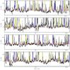 |
Fig. B.5 Synthetic spectra (red: (CH2OH)2, yellow: HCOOCH3, green: CH2OHCHO, blue: the molecules listed in Table A.1) on top of observed spectrum (black) at 3 mm for W51/e2 in the frequency range ~100–103 GHz. |
 |
Fig. B.7 Synthetic spectra (red: (CH2OH)2, yellow: HCOOCH3, green: CH2OHCHO, blue: the molecules listed in Table A.1) on top of observed spectrum (black) at 3 mm for G34.3+0.2 in the frequency range ~100–103 GHz. |
Acknowledgments
We would like to thank the referee, Malcolm Walmsley, for his help improving the paper. The research of J.M.L. and J.K.J. was supported by a Junior Group Leader Fellowship from the Lundbeck Foundation to J.K.J., – as well as the Centre for Star and Planet Formation funded by the Danish National Research Foundation. C.F. acknowledges support from the National Science Foundation under grant 1008800.
References
- Aikawa, Y., Wakelam, V., Garrod, R. T., & Herbst, E. 2008, ApJ, 674, 984 [NASA ADS] [CrossRef] [Google Scholar]
- Beltrán, M. T., Codella, C., Viti, S., Neri, R., & Cesaroni, R. 2009, ApJ, 690, L93 [NASA ADS] [CrossRef] [Google Scholar]
- Bisschop, S. E., Jørgensen, J. K., van Dishoeck, E. F., & de Wachter, E. B. M. 2007, A&A, 465, 913 [NASA ADS] [CrossRef] [EDP Sciences] [Google Scholar]
- Biver, N., Bockelée-Morvan, D., Debout, V., et al. 2014, A&A, 566, L5 [Google Scholar]
- Blake, G. A., Sutton, E. C., Masson, C. R., & Phillips, T. G. 1987, ApJ, 315, 621 [NASA ADS] [CrossRef] [Google Scholar]
- Bockelée-Morvan, D., Lis, D. C., Wink, J. E., et al. 2000, A&A, 353, 1101 [NASA ADS] [Google Scholar]
- Brouillet, N., Despois, D., Lu, X.-H., et al. 2015, A&A, 576, A129 [NASA ADS] [CrossRef] [EDP Sciences] [Google Scholar]
- Carroll, P. B., Drouin, B. J., & Widicus Weaver, S. L. 2010, ApJ, 723, 845 [NASA ADS] [CrossRef] [Google Scholar]
- Charnley, S. B., Tielens, A. G. G. M., & Millar, T. J. 1992, ApJ, 399, L71 [NASA ADS] [CrossRef] [Google Scholar]
- Christen, D., Coudert, L. H., Suenram, R. D., & Lovas, F. J. 1995, J. Mol. Spectr., 172, 57 [NASA ADS] [CrossRef] [Google Scholar]
- Christen, D., & Müller, H. S. P. 2003, Phys. Chem. Chem. Phys., 5, 3600 [Google Scholar]
- Coutens, A., Persson, M. V., Jørgensen, J. K., Wampfler, S. F., & Lykke, J. M. 2015, A&A, 576, A5 [NASA ADS] [CrossRef] [EDP Sciences] [Google Scholar]
- Crockett, N. R., Bergin, E. A., Neill, J. L., et al. 2014, ApJ, 781, 114 [NASA ADS] [CrossRef] [Google Scholar]
- Crovisier, J., Bockelée-Morvan, D., Biver, N., et al. 2004a, A&A, 418, L35 [NASA ADS] [CrossRef] [EDP Sciences] [Google Scholar]
- Crovisier, J., Bockelée-Morvan, D., Colom, P., et al. 2004b, A&A, 418, 1141 [NASA ADS] [CrossRef] [EDP Sciences] [Google Scholar]
- Demyk, K., Wlodarczak, G., & Carvajal, M. 2008, A&A, 489, 589 [NASA ADS] [CrossRef] [EDP Sciences] [Google Scholar]
- Favre, C., Despois, D., Brouillet, N., et al. 2011, A&A, 532, A32 [NASA ADS] [CrossRef] [EDP Sciences] [Google Scholar]
- Favre, C., Carvajal, M., Field, D., et al. 2014, ApJS, 215, 25 [NASA ADS] [CrossRef] [Google Scholar]
- Fuente, A., Cernicharo, J., Caselli, P., et al. 2014, A&A, 568, A65 [NASA ADS] [CrossRef] [EDP Sciences] [Google Scholar]
- Garrod, R. T., Weaver, S. L. W., & Herbst, E. 2008, ApJ, 682, 283 [NASA ADS] [CrossRef] [Google Scholar]
- Geppert, W. D., Hamberg, M., Thomas, R. D., et al. 2006, Faraday Discussions, 133, 177 [Google Scholar]
- Goldsmith, P. F., & Langer, W. D. 1999, ApJ, 517, 209 [NASA ADS] [CrossRef] [Google Scholar]
- Goldsmith, P. F., Lis, D. C., Hills, R., & Lasenby, J. 1990, ApJ, 350, 186 [NASA ADS] [CrossRef] [Google Scholar]
- Halfen, D. T., Apponi, A. J., Woolf, N., Polt, R., & Ziurys, L. M. 2006, ApJ, 639, 237 [NASA ADS] [CrossRef] [Google Scholar]
- Herbst, E., & van Dishoeck, E. F. 2009, ARA&A, 47, 427 [NASA ADS] [CrossRef] [Google Scholar]
- Hollis, J. M., Lovas, F. J., & Jewell, P. R. 2000, ApJ, 540, L107 [NASA ADS] [CrossRef] [Google Scholar]
- Hollis, J. M., Vogel, S. N., Snyder, L. E., Jewell, P. R., & Lovas, F. J. 2001, ApJ, 554, L81 [Google Scholar]
- Hollis, J. M., Lovas, F. J., Jewell, P. R., & Coudert, L. H. 2002, ApJ, 571, L59 [NASA ADS] [CrossRef] [Google Scholar]
- Hollis, J. M., Jewell, P. R., Lovas, F. J., & Remijan, A. 2004, ApJ, 613, L45 [NASA ADS] [CrossRef] [Google Scholar]
- Ilyushin, V., Kryvda, A., & Alekseev, E. 2009, J. Mol. Spectr., 255, 32 [NASA ADS] [CrossRef] [Google Scholar]
- Jørgensen, J. K., van Dishoeck, E. F., Visser, R., et al. 2009, A&A, 507, 861 [NASA ADS] [CrossRef] [EDP Sciences] [Google Scholar]
- Jørgensen, J. K., Favre, C., Bisschop, S. E., et al. 2012, ApJ, 757, L4 [NASA ADS] [CrossRef] [Google Scholar]
- Kalenskii, S. V., & Johansson, L. E. B. 2010, Astron. Rep., 54, 1084 [NASA ADS] [CrossRef] [Google Scholar]
- Kurtz, S., Cesaroni, R., Churchwell, E., Hofner, P., & Walmsley, C. M. 2000, Protostars and Planets IV, 299 [Google Scholar]
- Maury, A. J., Belloche, A., André, P., et al. 2014, A&A, 563, L2 [NASA ADS] [CrossRef] [EDP Sciences] [Google Scholar]
- Millar, T. J., Herbst, E., & Charnley, S. B. 1991, ApJ, 369, 147 [NASA ADS] [CrossRef] [Google Scholar]
- Müller, H. S. P., Thorwirth, S., Roth, D. A., & Winnewisser, G. 2001, A&A, 370, L49 [NASA ADS] [CrossRef] [EDP Sciences] [Google Scholar]
- Müller, H. S. P., Schlöder, F., Stutzki, J., & Winnewisser, G. 2005, J. Mol. Str., 742, 215 [CrossRef] [Google Scholar]
- Öberg, K. I., Garrod, R. T., van Dishoeck, E. F., & Linnartz, H. 2009, A&A, 504, 891 [NASA ADS] [CrossRef] [EDP Sciences] [Google Scholar]
- Öberg, K. I., Boogert, A. C. A., Pontoppidan, K. M., et al. 2011, ApJ, 740, 109 [NASA ADS] [CrossRef] [Google Scholar]
- Pickett, H. M., Poynter, I. R. L., Cohen, E. A., et al. 1998, J. Quant. Spectr. Radiat. Trans., 60, 883 [Google Scholar]
- Remijan, A., Snyder, L. E., Friedel, D. N., Liu, S.-Y., & Shah, R. Y. 2003, ApJ, 590, 314 [NASA ADS] [CrossRef] [Google Scholar]
- Requena-Torres, M. A., Martín-Pintado, J., Martín, S., & Morris, M. R. 2008, ApJ, 672, 352 [NASA ADS] [CrossRef] [Google Scholar]
- Sato, M., Reid, M. J., Brunthaler, A., & Menten, K. M. 2010, ApJ, 720, 1055 [NASA ADS] [CrossRef] [Google Scholar]
- Schöier, F. L., Jørgensen, J. K., van Dishoeck, E. F., & Blake, G. A. 2002, A&A, 390, 1001 [NASA ADS] [CrossRef] [EDP Sciences] [Google Scholar]
- Taquet, V., López-Sepulcre, A., Ceccarelli, C., et al. 2015, ApJ, 804, 81 [NASA ADS] [CrossRef] [Google Scholar]
- Urquhart, J. S., Figura, C. C., Moore, T. J. T., et al. 2014, MNRAS, 437, 1791 [NASA ADS] [CrossRef] [Google Scholar]
- van Dishoeck, E. F., Kristensen, L. E., Benz, A. O., et al. 2011, PASP, 123, 138 [NASA ADS] [CrossRef] [Google Scholar]
- Viti, S., Collings, M. P., Dever, J. W., McCoustra, M. R. S., & Williams, D. A. 2004, MNRAS, 354, 1141 [NASA ADS] [CrossRef] [Google Scholar]
- Zhang, Q., Ho, P. T. P., & Ohashi, N. 1998, ApJ, 494, 636 [NASA ADS] [CrossRef] [Google Scholar]
All Tables
Transitions of (CH2OH)2 observed toward W51/e2 and G34.3+0.2 with the IRAM 30–m telescope.
All Figures
|
Fig. 1 Observed (black) and synthetic (red) spectra of the five transitions of (CH2OH)2 in W51/e2 that are used for the analysis. Also shown are the synthetic spectra of all other species investigated in this study (blue) to demonstrate that the (CH2OH)2 lines in question are not blended. The transitions are located at 239 883.56, 240 807.88, 242 656.23, 242 948.29 and 100 333.64 MHz – denoted by black vertical lines in the plot. The displayed frequency region in each plot corresponds to ~200 km s-1. |
| In the text | |
|
Fig. 2 Same as for Fig. 1 but for G34.3+0.2. The transitions are located at 240 807.88 and 242 656.23 MHz – indicated by black vertical lines in the plot. |
| In the text | |
|
Fig. 3 Schematic bar plot of HCOOCH3/CH2OHCHO (top) and HCOOCH3/(CH2OH)2 (bottom) against Lbol. The sources from Table 4 have been plotted in descending order of luminosity from left to right on the x-axis, but not to scale, and the sources have been grouped into high-mass sources (blue), intermediate-mass protostar (red) and low-mass protostars (green). The white bars for four of the high-mass sources are upper or lower levels, which is indicated by the direction of the arrow. The luminosity for the top plot spans from Sgr B2(N) with Lbol = 107L⊙ to IRAS NGC 1333 4A with Lbol = 7.7 L⊙, while it spans from W51/e2 with Lbol = 4.7 × 10⁶L⊙ to IRAS NGC 1333 4A with Lbol = 20 L⊙ in the bottom plot. |
| In the text | |
|
Fig. B.1 Synthetic spectra (red: (CH2OH)2, yellow: HCOOCH3, green: CH2OHCHO, blue: the molecules listed in Table A.1) on top of observed spectrum (black) at 1 mm for W51/e2 in the frequency range ~238–242 GHz. |
| In the text | |
 |
Fig. B.2 Same as Fig. B.1 but for ~242–246 GHz. |
| In the text | |
|
Fig. B.3 Synthetic spectra (red: (CH2OH)2, yellow: HCOOCH3, green: CH2OHCHO, blue: the molecules listed in Table A.1) on top of observed spectrum (black) at 1 mm for G34.3+0.2 in the frequency range ~238–242 GHz. |
| In the text | |
 |
Fig. B.4 Same as for Fig. B.3 but for ~242–246 GHz. |
| In the text | |
|
Fig. B.5 Synthetic spectra (red: (CH2OH)2, yellow: HCOOCH3, green: CH2OHCHO, blue: the molecules listed in Table A.1) on top of observed spectrum (black) at 3 mm for W51/e2 in the frequency range ~100–103 GHz. |
| In the text | |
 |
Fig. B.6 Same as for Fig. B.5 but for ~103–106 GHz. |
| In the text | |
|
Fig. B.7 Synthetic spectra (red: (CH2OH)2, yellow: HCOOCH3, green: CH2OHCHO, blue: the molecules listed in Table A.1) on top of observed spectrum (black) at 3 mm for G34.3+0.2 in the frequency range ~100–103 GHz. |
| In the text | |
 |
Fig. B.8 Same as for Fig. B.7 but for ~103–106 GHz. |
| In the text | |
Current usage metrics show cumulative count of Article Views (full-text article views including HTML views, PDF and ePub downloads, according to the available data) and Abstracts Views on Vision4Press platform.
Data correspond to usage on the plateform after 2015. The current usage metrics is available 48-96 hours after online publication and is updated daily on week days.
Initial download of the metrics may take a while.