| Issue |
A&A
Volume 582, October 2015
|
|
|---|---|---|
| Article Number | A104 | |
| Number of page(s) | 13 | |
| Section | The Sun | |
| DOI | https://doi.org/10.1051/0004-6361/201526124 | |
| Published online | 20 October 2015 | |
Multiwavelength spectropolarimetric observations of an Ellerman bomb
1 Kiepenheuer-Institut für Sonnenphysik, Schöneckstr. 6, 79104 Freiburg, Germany
e-mail: This email address is being protected from spambots. You need JavaScript enabled to view it.
2 National Solar Observatory (NSO), 3010 Coronal Loop, 88349 Sunspot, New Mexico, USA
e-mail: This email address is being protected from spambots. You need JavaScript enabled to view it.
Received: 18 March 2015
Accepted: 14 August 2015
Abstract
Context. Ellerman bombs (EBs) are enhanced emission in the wings of the Hα line in the solar spectrum.
Aims. We study the structure of an EB in the photosphere and chromosphere.
Methods. We analyze simultaneous observations of four chromospheric lines (Hα, Ca ii H, Ca ii IR 854 nm, and He i 1083 nm) as well as two photospheric lines (Fe i 630 and Si i 1082.7 nm) along with high-cadence 160 and 170 nm ultraviolet (UV) continuum filtergrams. Full Stokes data from the Helioseismic and Magnetic Imager (HMI) are used to trace the temporal evolution of the magnetic structure.
Results. We identify the EB by excess emission in the wings of the Hα line, a brightening in the UV continuum, and large emission peaks in the core of the two Ca ii lines. The EB shows a blueshift in all chromospheric lines, while no shifts are observed in the photospheric lines. The blueshift in the chromospheric layer causes very asymmetric emission peaks in the Ca ii H line. The photospheric Si i spectral line shows a shallower line depth at the location of the EB. The UV continuum maps show that the EB was substantially brighter than its surroundings for about 30 min. The continuum contrast of the EB from 170 nm to 1080 nm shows a power-law dependency on the wavelength. The temperature enhancement amounts to 130 K in the low photosphere and 400 K at the temperature minimum level. This temperature excess is also seen in an LTE inversion of the Ca ii spectra. The total thermal and radiative energy content of the EB is about 1020 J and 1018 J in the photosphere and chromosphere, respectively. The HMI data hints at a photospheric magnetic flux cancellation as the driver of the EB.
Conclusions. Ellerman bombs release the energy in a height range of several pressure scale heights around the temperature minimum such that they affect both the photosphere and the lower chromosphere.
Key words: Sun: photosphere / Sun: chromosphere / Sun: magnetic fields / sunspots / Sun: infrared / Sun: UV radiation
© ESO, 2015
1. Introduction
Ellerman (1917) first reported short-lived brightenings in the wing of the Hα line which were not conspicuous in the line-core emission, known later on as Ellerman bombs (EBs). These intensity enhancements are symmetric on both sides of the line core. Subsequent observations showed that a majority of EBs have a blue asymmetry in the Hα line profile (Bruzek 1972). Extended brightenings in the wings of strong chromospheric lines like Hα, Ca ii, or Mg ii are referred to as moustaches (Severny 1957). Ellerman bombs and moustaches are different names for the same phenomena (McMath et al. 1960; Severny 1968; Bruzek 1972). They usually appear in areas of emerging magnetic flux, around sunspots, in network regions, and at neutral lines (Kurokawa et al. 1982; Dara et al. 1997); they have a fractal nature, clustering at network boundaries and in areas of flux emergence (Georgoulis et al. 2002). Some studies made a link between EBs and undulating field topologies in emerging flux regions (Pariat et al. 2004; Watanabe et al. 2008). Bello González et al. (2013) found evidence for the existence of opposite magnetic polarities at the sites of three EBs.
Ellerman bombs have a typical lifetime of a few minutes, but can live up to an hour (Kurokawa et al. 1982; Georgoulis et al. 2002; Pariat et al. 2007; Bello González et al. 2013). The brightening peaks at about Hα ± 1.2 Å and fades away toward ±5 Å (Berlicki et al. 2010; Kneer 2010). This excess emission corresponds to a temperature enhancement of 600 to 2000 K at about the height of the temperature minimum (Georgoulis et al. 2002; Fang et al. 2006; Hong et al. 2014). These structures are a few arcsec in size and usually show an elongated shape (Rutten et al. 2013). They are hot structures embedded in the upper photosphere and lower chromosphere. They usually show an enhanced brightness in the continuum and strong vertical polarization signals. Some authors have attributed an energy content of about ~ 1019−21 J to EBs and have suggested reconnection as their triggering mechanism (Payne 1993; Georgoulis et al. 2002). The symmetric temporal profile of EBs (Payne 1993; Qiu et al. 2000; Berlicki et al. 2010) is different from that of flare-like events which have a short rise time and a longer decay time. This causes a problem in attributing EBs to small-scale events like nanoflares (Parker 1988).
From limb data, Harvey (1963) reported that EBs are placed at a height of 400 km above the photosphere. Payne (1993), Berlicki et al. (2010), and Bello González et al. (2013) found them to lie around the temperature minimum and above it. Some authors suggested that EBs form in the low chromosphere (Matsumoto et al. 2008), while others found that they are solely a photospheric phenomena (Watanabe et al. 2011; Vissers et al. 2013).
There is an ambiguity in the exact definition of EBs. While some authors found them to be co-spatial with facular features and network bright points (Bruzek 1972; Kitai & Muller 1984; Stellmacher & Wiehr 1991), others argued that not every brightening in the wing of Hα line is a signature of EBs (Watanabe et al. 2011; Rutten et al. 2013). For instance, the EBs shown by Roy & Leparskas (1973) match fairly well with the ones shown by Pariat et al. (2007). However, it is not clear if these objects are indeed the same features reported by Ellerman (1917) or Socas-Navarro et al. (2006). The profiles in the former case show an enhanced emission in the Hα line wing that amounts to a small percentage (in units of the continuum intensity), while in the latter case, the excess emission is substantial. The number of EBs observed by different people also suggests a different nature for the events. Nelson et al. (2013), for instance, used imaging spectroscopy and reported 3500 EBs around a sunspot in 90 min while Bello González et al. (2013) used the same observational technique and reported only three EBs in 130 min. Therefore, there is an uncertainty in distinguishing between EBs and magnetic bright points in the literature (Rutten et al. 2013).
The spectropolarimetric signatures of EBs have been observed in Ca ii IR lines by Socas-Navarro et al. (2006), who found strongly redshifted Ca ii IR line profiles in the moat of a sunspot. There are indications that some EBs are essentially moving magnetic features (Harvey & Harvey 1973) in the moat of sunspots (e.g., Nindos & Zirin 1998). Fang et al. (2006) and Pariat et al. (2007) found signatures of EBs in the Ca ii IR lines and in Hα. These studies showed that EBs exhibit enhanced brightenings not only in the wing of the Hα line, but also in the wings of the Ca ii IR line. Traces of EBs were also observed in the ultraviolet (UV) continuum at 160 nm (Qiu et al. 2000; Pariat et al. 2007), while Hashimoto et al. (2010) observed EBs in the Ca ii H line.
Ellerman bombs correspond to upflows in the middle/lower chromosphere, but mostly downflows in the photosphere. Socas-Navarro et al. (2006) reported a strong redshift (>10 km s-1) in the wing of the Ca ii IR line. In their inversions, they found that EBs can be either hotter or cooler than the surrounding atmosphere. Watanabe et al. (2011) mostly found a simultaneous redshift in the photosphere and a blueshift in the chromosphere, but sometimes found the reverse configuration.
 |
Fig. 1 Overview maps of the observed area. Top row, left to right: the intensity of the Ca ii H pseudo-continuum in the far blue wing, the outer and inner wing intensities, and the line-core intensity (H3). Middle row: the intensity of the Ca ii IR continuum, the monochromatic intensity at −10 and +5 pm from the line core, and the line-core intensity. Bottom row: the Si i continuum intensity, the polarization degree from the POLIS Fe i 630 nm data, the Si i line-core intensity, and the He i line-core intensity. The intensity maps are normalized to the nearby continuum intensity of the average quiet Sun. The contour and circle outline a magnetic field strength of 700 G and the location of the EB, respectively. The arrow marks the direction of disk center. |
In this paper, we investigate the thermal and magnetic properties of an energetic event and attribute it to an EB. We present the signatures of an EB in the spectral lines of Ca ii H and He i 1083 nm in addition to the commonly used lines of Hα and Ca ii IR. The observations and the data reduction are described in Sects. 2 and 3, respectively. Our results are presented in Sect. 4 and discussed in Sect. 5, while our conclusions are given in Sect. 6.
2. Observations
The leading sunspot in active region NOAA 11191 at a heliocentric angle of 70° was observed at the German Vacuum Tower Telescope (VTT, Schröter et al. 1985) in Tenerife on April 13, 2011, from 07:49–08:15 UTC. The good and stable seeing conditions during the observation and the Kiepenheuer-Institut Adaptive Optics System (von der Lühe et al. 2003; Berkefeld et al. 2010) provided a spatial resolution of about 1′′.We combined the Tenerife Infrared Polarimeter (TIP II; Martínez Pillet et al. 1999; Collados et al. 2007) attached to the Echelle spectrograph, the POlarimetric LIttrow Spectrograph (POLIS; Schmidt et al. 2003; Beck et al. 2005b), and two additional channels to record the intensity spectra of the Ca ii IR line via the Echelle spectrograph and Hα intensity profiles via POLIS. A dichroic beam-splitter was used to feed POLIS with visible light and TIP with infrared light. More details of the setup can be found in Beck & Rezaei (2012; see also Beck et al. 2007 or Kucera et al. 2008 for a similar combination using TIP and TESOS).
Summary of observations.
2.1. Infrared spectropolarimetric data
The TIP recorded full Stokes profiles of the spectral lines Si i 1082.7 nm and He i 1083.0 nm. A slit width corresponding to 0.̋36 and a step size of 0.̋36 were used to scan a range of 54′′ with a slit length of 78′′. The spatial sampling along the slit (after binning) was  . The spectral sampling was 1.1 pm and the integration time per slit position was 6 s. The polarimetric calibration was performed using the VTT telescope model and the near-IR instrumental calibration unit (Beck et al. 2005a). The residual crosstalk was corrected with the statistical method of Schlichenmaier & Collados (2002). The 1σ noise level in the TIP data is about 1.9 × 10⁻³Ic.
As discussed above, we also simultaneously recorded the Ca ii IR 854.2 nm intensity profile. The data has the same spectral and spatial sampling as in the case of TIP. The reduction procedures are discussed in Beck & Rezaei (2012).
2.2. Visible spectral data
The Ca ii H intensity profile and Stokes vector profiles of the visible Fe i lines at 630.15 nm and 630.25 nm were observed with the blue and red channels of the POLIS, respectively. POLIS used an integration time of about 4.8 s per slit position. Details of the calibration procedure for the calcium profiles are explained in Beck et al. (2005b). An additional camera was installed to record Hα spectra. A spectral range of 2 nm around the Hα line core was recorded. A standard data calibration procedure was applied to the Hα data (dark current correction, flat field). The calibrated spectra were corrected for the order-selecting prefilter by comparing the average quiet Sun profile (at disk center) to the FTS profile (Kurucz et al. 1984). The slit height in the Hα raster scans was about 160′′, which is larger than the 90 (70)′′ in the POLIS red (blue) channel.
2.3. Correction for scattered light
We used the method of Beck et al. (2011) to remove the scattered light from the Ca ii H data. As discussed by Rezaei et al. (2007a), the amount of scattered light in the red channel of POLIS is negligible, compared to the blue channel. Hence, we did not apply any correction to other spectral lines but Ca ii H.
2.4. Data alignment
The continuum map in each channel was used to compensate for the differential refraction in the Earth’s atmosphere (Filippenko 1982; Reardon 2006; Beck et al. 2008; Felipe et al. 2010). To this end, the same method as in Beck et al. (2008) was applied to the data. After that, all maps were aligned to the Ca ii H map, which has the smallest field of view.
Figure 1 shows an overview of the observed region after the alignment. The chosen wavelengths in the Ca ii H line (top row; see Table 1 of Rezaei et al.2007a) trace the intensity variation from continuum-forming layers through the middle and upper photosphere up to the chromosphere (Cram & Damé 1983; Lites et al. 1993; Rezaei et al. 2007a). The middle row shows the continuum, blue and red wing intensities, and the line-core emission of the Ca ii IR line that sample similar heights. The dashed circle marks an area with explosive characteristics (large intensity at intermediate wavelengths between continuum and line core, blueshift in chromospheric lines). Compared to the Ca ii H line, the excess emission in Ca ii IR is at a wavelength closer to the core of the line. In the next section, we discuss the brightening in detail and identify it as an EB.
 |
Fig. 2 AIA data. Top row: filtergrams at 160 and 170 nm co-temporal with the profiles shown in Fig. 9. For a description of the contour and circle, see Fig. 1. Bottom panel: temporal variation of the intensity of the EB in AIA 160 and 170 nm images. The vertical lines mark the time span of the VTT observations. The red line marks the time at which the the slit passed across the EB. |
The Si i 1083 nm continuum and line-core intensities, the polarization degree in the photosphere derived from the Fe i 630 nm line, and the line-core intensity of the He i 1083 nm line are shown in the bottom row of Fig. 1. Magnetic structures seen in the map of the photospheric polarization degree have a higher contrast in the pseudo-continuum map of Ca ii H line (top left panel) compared to the near-infrared (IR) continuum (bottom left panel). There is significant polarization signal at the location of the EB. The EB shows up in the Si i line-core intensity, but is not clearly seen in the core of the He i 1083 nm line.
2.5. AIA 160/170 nm data
Simultaneous UV maps at 160 nm and 170 nm from the Atmospheric Imaging Assembly (AIA; Lemen et al. 2012) on board the Solar Dynamics Observatory (SDO, Pesnell et al. 2012) were reduced and aligned using SolarSoft. This was motivated by the fact that several authors have already used UV maps as tracer of EBs. The 170 nm continuum emission forms at about the temperature minimum (Vernazza et al. 1981). In contrast, the 160 nm data has a mixed signal both from the upper photosphere and the transition region: the light transmitted in this filter originates from the 160 nm continuum, but has some contamination from strong emission lines (Judge 2006; Vissers et al. 2013).
Two aligned maps with overlayed contours of the photospheric field strength are shown in the top row of Fig. 2, which shows that the EB is clearly brighter than its nearby surroundings. The temporal evolution of the intensity inside the circle in the AIA data (bottom panel of Fig. 2) shows that the EB had dropped to about half of its maximum intensity at the time when the slit was passing over the region. The UV brightening lasted for about 30 min.
2.6. HMI spectropolarimetric data
We gathered simultaneous Stokes maps of the Helioseismic and Magnetic Imager (HMI, Scherrer et al. 2012; Schou et al. 2012), a filter spectropolarimeter on board the SDO. The HMI data in this study lasts from 07:00 to 08:36 UTC with a cadence of 12 min. The spatial resolution of HMI maps is one arcsecond, which is comparable to our VTT data.
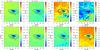 |
Fig. 3 The Ellerman bomb in the Hα line. All values are in units of the continuum intensity of the average quiet Sun profile at 656 nm. For a description of the contour and circle, see Fig. 1. |
3. Data analysis
3.1. Line parameters
Line-wing and line-core intensities, and line-core velocities were determined for all strong chromospheric lines (Hα, Ca ii H, Ca ii IR). We also determined the ratio of the violet and red emission peaks of the Ca ii H line and the center of gravity of the intensity at the Ca ii H line core as velocity proxies.
3.2. Inversion of spectropolarimetric data
The spectropolarimetric data of Si i 1082.7 nm were inverted with the SIR code (Stokes Inversion based on Response functions; Ruiz Cobo & del Toro Iniesta 1992; Bellot Rubio 2003). We only used one node for all parameters except for the temperature (e.g., Beck 2008; Rezaei et al. 2012). The magnetic field vector, the line-of-sight (LOS) velocity and temperature stratifications were retrieved from the inversion.
We used the Helium Line Information Extractor plus (HeLIx+) code (Lagg et al. 2004; Lagg 2007) to retrieve the chromospheric magnetic field parameters from the helium line. We also simultaneously inverted the Si i line which returned the same results as the SIR code (see Borrero et al.2014 for a detailed comparison of the two codes).
We inverted the Stokes profiles from HMI using the Very Fast Inversion of the Stokes Vector (VFISV, Borrero et al. 2007, 2011) code to retrieve the magnetic field vector in the photosphere (see Kiess et al.2014 for a detailed explanation of the inversion setup). The retrieved magnetic field vector was transformed into the local reference frame. This was necessary because it would have been impossible to see any small opposite-polarity patches in a simple LOS magnetogram given the large heliocentric angle of the observations. The intrinsic 180° ambiguity in the magnetic field azimuth (Metcalf 1994; Lites et al. 1995) was resolved using the AZAM code (Elmore et al. 1992; Tomczyk et al. 1992; Metcalf et al. 2006).
3.3. Identification of EBs
Almost all of the observed wavelength bands of the two Ca ii lines show an intensity enhancement in the core and wing at the location of the possible EB (Fig. 1). An inspection of the photospheric temperature obtained in SIR inversion also showed enhanced temperatures at all heights.
To identify any other EBs, we evaluated the Hα and Ca ii IR line wing intensities. The Hα line is widely used as a tracer of EBs, although there is no one-to-one correspondence between brightenings in the wing of this line and EBs. Figure 3 shows the observed region at four wavelengths (80, 120, and 160 pm from the line core) in the blue wing (top row) and the red wing (bottom row). The line-core and a red-wing intensity at 320 pm are shown in the right column. Any small-scale intensity enhancement in a line-wing map could indicate an EB.
We limited the candidates by comparing the selected line profiles with average quiet Sun profiles. As shown by Pariat et al. (2007, their Fig. 10), the difference profile exhibits the same pattern as a regular Stokes Q profile. We found only one prominent example inside our field of view (FOV) in which a Stokes Q-like difference profile of Hα was observed, located at the place of the increased intensity in the Ca ii (Fig. 1) and UV data (Fig. 2). In the Hα maps of Fig. 3, the EB is best seen in a range of ±80−160 pm around the line core. However, it remains brighter than the nearby continuum in a wavelength range of several Angstroms. The excess emission is symmetric with respect to the line core: the EB is seen both in the blue and red wings. These parameters are sufficient to identify it as an EB (Rutten et al. 2013). As seen in Figs. 1 and 2, the EB is elongated as reported in earlier observations (e.g., Georgoulis et al. 2002). The line-wing images in Fig. 3 and the analysis of the spectral shape showed no other EB inside our field of view.
The line-core intensity of Hα (top right panel of Fig. 3) is enhanced at the location of the EB, but this is most likely not related to the EB itself. The increase of the line-core intensity affects an extended area around the EB that shows loop-like structures. The line-core intensity is not larger than, for instance, in the network region at the lower boundary of the FOV, contrary to the appearance of the EB in the Hα line-wing images. As can be seen in the spectra shown in the top row of Fig. 9, there is a wide emission band on either side of the Hα line core in the EB which has an intensity larger than the nearby continuum. The intensity of the Hα line core itself is only slightly higher in the EB than in a quiet Sun reference profile. In other words, the core of the Hα line at the location of the EB is slightly elevated but still in absorption, while the line wings are in emission.
Evaluating 437 full-disk HMI magnetograms between April 12 and 15, we find that the active region (AR) had episodes of flux emergence during this time interval. The flux emergence clearly continued after the formation of sunspots in the AR. This supports the identification as an EB since EBs are mostly observed in flux emergence areas and close to neutral lines.
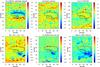 |
Fig. 4 Velocity maps. Top, left to right: the absolute line-core velocity of Fe i 630.25 nm line, line-core velocity of Si i 1082.7 nm line retrieved via SIR inversion, and Ca ii H center-of-gravity velocity. Bottom, left to right: Hα, Ca ii IR line-core, and He i 1083 nm line-core velocity obtained by the HeLIx+ inversion. The center-of-gravity velocity of Ca ii H line was calculated for a spectral range of 100 pm around the line core. All velocities are in km s-1. |
4. Results
4.1. Doppler shifts associated with the EB
The LOS velocities of different lines are shown in Fig. 4. The photospheric line-core velocity of the Fe i 630.15 nm line was calibrated using the nearby telluric lines (Balthasar et al. 1982; Rezaei et al. 2006). This map (top left panel) shows a similar pattern to the velocity retrieved from the inversion of the Si i line (top middle panel). There is no significant Doppler shift in the photospheric lines at the location of the EB.
 |
Fig. 5 Left to right: photospheric magnetic field strength from SIR inversion (G), chromospheric magnetic field strength from HeLIx+ inversion (G), and the LRF inclination maps of HMI data at 07:00 and 08:12 (deg). For a description of the contour and circle, see Fig. 1. |
The top right panel shows the center-of-gravity (COG) velocity of the Ca ii H line in a 0.1 nm band around the line core. This map more closely resembles the chromospheric line-core velocities of the Hα, Ca ii IR, and He i 1083 nm lines in the bottom row than the two photospheric velocities in the top panel. All four chromospheric velocity maps show a blueshift co-spatial to the location of the EB. The blueshifts are largest in the helium line (up to 40 km s-1) and often larger than 10 km s-1, although at a heliocentric angle of 70°, a blueshift is more a horizontal velocity than an upflow. Hence, it is not straightforward to attribute them to the EB, although as we discuss below, an upflow would be consistent with a magnetic flux cancellation event. The velocity map of, for example, the Hα line-core velocity (bottom-left panel, Fig. 4), shows loop-like structures near the EB that perhaps cover the lower layers. The same pattern is also seen for the line-core velocity of the Ca ii IR, and He i 1083 nm lines. We note the large velocity scale in comparison to the photospheric velocities.
4.2. Chromospheric loops
As seen in Fig. 4, the EB is co-spatial with a blueshift in all chromospheric lines.
All chromospheric velocity maps show loop-like structures. These blueshifts are a mixture of loops and the EB. The blueshift in the COG of Ca ii H line most probably indicates an upflow in the lower chromosphere. The same loops seen in the Hα line-core velocity map are also seen in Ca ii H, helium, and Hα line-core intensities (Figs. 1 and 3). These loops connect the sunspot with the opposite polarity in this active region which is located at the bottom of the maps (see the polarization degree map in the bottom row of Fig. 1).
No signature of the EB is seen in the helium or Hα line-core maps while both Ca ii lines show a brighter line-core intensity than in a quiet Sun profile. The bright patches in the Hα line-core intensity map have a different pattern compared to the EB seen in the wing maps. This indicates that the EB forms at a lower height than the formation height of the helium or Hα lines and is embedded in the lower atmosphere, as already known. The velocity map of the helium line is a result of the HeLIx+ inversion (Sect. 3.2).
4.3. Signature of a magnetic flux cancellation
There is a significant polarization signal in the photospheric area of the EB (Fig. 1). The photospheric magnetic field strength retrieved from the SIR inversion (Fig. 5) amounts to 680 ± 150 G (the error shows the dispersion of values). This can be compared with the chromospheric field strength retrieved from the HeLIx+ inversion which amounts to 460 ± 70 G. Both in the photosphere and chromosphere, the field lines are inclined, i.e., there are significant Stokes Q and U profiles.
The magnetic flux map in the local reference frame from the VFISV inversion at 07:00 UTC shows a patch of magnetic flux with an orientation opposite to that of the sunspot close to the EB location. This patch has completely disappeared at 08:12 UTC (Fig. 5). The temporal evolution of the region is shown in magnified cut-outs from the inversion results in Fig. 6. The opposite-polarity patch reached its largest extent at 07:24 UTC, slightly before the time when the AIA UV intensities peaked (Fig. 2). The frames at 07:48 and 08:00 UTC show little to no trace of an opposite polarity above 200 G, especially in the inclination map (top row of Fig. 6). This indicates the cancellation of the magnetic flux, although the temporal cadence does not allow a 1−1 correspondence to be attributed to the event recorded in the spectrograph data at about 7:56 UTC (Fig. 9).
 |
Fig. 6 Magnetic field inclination (top) and flux (bottom) in the local reference frame from HMI data with 12-min cadence. Time increases from left to right between 7:00 and 8:36. The contour, circle, and coordinates are as in the full maps (Figs. 1, 3–5). The yellow patch seen in the center of the circle at left in the flux maps disappears gradually. Inclination is in degrees and flux in G. |
4.4. Continuum contrast of the EB as a function of wavelength
We followed the temporal evolution of the EB in the AIA filtergrams from 07:00 to 08:30 UTC. Figure 2 shows the light curve of the maximum (solid) and the mean (dashed) emission inside the circle marked in Fig. 1 that outlines the EB. The mean value of a quiet Sun area (in the upper part of the map) is also plotted for comparison. It shows that the variation of the EB is not due to thermal instability, misalignment, or similar instrumental artifacts, but has a solar origin. The excess emission lasted for about half an hour. The VTT observations did not catch the maximum intensity in the AIA filtergrams, which was about a factor of two larger than when the slit passed over the EB.
An enhanced continuum intensity was still observed in all spectral channels recorded at the VTT. At the longest wavelength (1083 nm), the EB continuum has a contrast of 3%. The enhancement in the continuum of the Ca ii IR line is about 6.5%. The 630 nm and Hα channels of POLIS both have a contrast of 10%, while the excess intensity in the wing of Ca ii H amounts to 30%. The trend of increasing intensity contrast with decreasing wavelength continues in the UV continuum, where in 170 nm images the EB has an intensity of about 2.3 times the mean nearby quiet Sun area. The contrast of 160 nm images, which contains signals of transition region emission lines, are about 5.9 times the average quiet Sun.
Figure 7 shows a double logarithm plot of the continuum contrast of the EB in the six wavelength bands. The solid line represents a power-law fit to all data points except the one at 160 nm. The intensity at 160 nm was not included in the fit for two reasons: a) the intensity in this filter has contamination from emission lines in the transition region and b) the continuum below 170 nm generally has a larger formation height than the continuum at longer wavelengths and represents a mixed signal from different layers (Judge 2006). The power-law fit reproduces the wavelength run of the contrast with reasonable accuracy.
We used two methods to estimate the corresponding increase in temperature. An order-of-magnitude estimate based on the Planck function yielded a temperature enhancement of about 120 ± 20 K at the continuum forming layer and about 400 ± 50 K at the height of the temperature minimum of about 500 km. For a more solid estimate of the temperature enhancement, we synthesized a set of HSRA-like atmospheres with the SIR code. We evaluated the continuum intensity in each wavelength range for a temperature enhancement of 0–1000 K in steps of 10 K. The thermodynamic temperature excess associated with the intensity increase in the 1083, 854, 630, and 397 nm continuum bands were 110, 140, 160, and 360 K, respectively. These numbers are in good agreement with those obtained based on the Planck function.
The infrared continuum forms at layers a few ten kilometers deeper than the visible continuum. The pseudo-continuum of Ca ii H line forms at about 100–200 km above the τ500 = 1 level (Fig. 5 in Rezaei et al. 2008). At a height of about 500 km where the 170 nm continuum forms (Vernazza et al. 1981), the temperature excess is larger than in the middle photosphere, and the temperature excess in the middle photosphere is larger than in the deep photosphere.
 |
Fig. 7 The log–log plot of the continuum contrast vs. wavelength. The 160 nm data, which has contamination from transition region emission line, was not used for the linear fit (solid line). Numbers next to each data point show the wavelength in nm. The error bar of Ca ii IR continuum is larger mainly due to uncorrected fringes. |
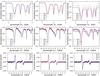 |
Fig. 8 Line profiles. Each row shows one spectral band. The three panels in each row show individual EB profiles (EB-1..7) along with a neighboring profile (EB-n) and the average quiet Sun profile. From top to bottom: the Fe i line pair at 630 nm, the He i 1083 nm and Si i 1082.7 nm Stokes I profile, and the corresponding Stokes V profile. The profiles are located inside the circle in Fig. 1 which outlines the EB. |
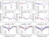 |
Fig. 9 Similar to Fig. 8 but for chromospheric lines. From top to bottom: the Hα line profile, the Ca ii H line profile, and the Ca ii IR intensity profile. We note the enhanced amplitude and width of the red emission peak pf Ca ii lines in the EB compared to the average quiet Sun profiles. The blueshift is clearly seen in the Hα line profile. |
4.5. Spectral line profiles
Figure 8 shows seven profiles of the EB along with average profiles of quiet Sun for the 630 nm range (top row) and Stokes I and Stokes V of the Si i and He i 1083 nm lines (middle and bottom row). A profile from a neighboring point in the vicinity of the EB is also shown for comparison (labeled EB-n in the legends). The increased continuum intensity is conspicuous in all panels of this figure, especially at 630 nm. The Si i line has a shallower line depth in the EB than in the average quiet Sun profile (middle row in Fig. 9). This is also clearly seen in the map of the line-core intensity of the Si i line (bottom row, Fig. 1). There is strong polarization signal in both the photospheric Si i and the chromospheric He i line.
The He i 1083 nm line usually has strong absorption co-spatial with the location of the EB and often shows its blue component. Interestingly, the Stokes V profile of this component in some cases is well above the noise level. This indicates that the LOS component of the magnetic field is strong enough at chromospheric heights to form such profiles (middle and bottom row of Fig. 8). We note, however, that a strong helium line is typical for active region areas, so it cannot be used as a stand-alone indicator of an EB.
Figure 9 is similar to Fig. 8 but for Hα (top row), Ca ii H (middle row), and Ca ii IR (bottom row). The emission peaks in the chromospheric lines are conspicuous in addition to the continuum contrast. The Hα line has a Stokes Q-like shape: two elevated wings and a dark core, similar to the ones reported in the literature (Vissers et al. 2013). The distance of the two emission features in the wings of Hα line is about 2.5 Å. The blue emission peak has an amplitude of 1.35 Ic, well above its continuum. The telluric line at about 6564.4 Å modified the shape of the red emission peak. The depth of the central minimum with respect to its own continuum is about twice as much as in a quiet Sun profile (top row, Fig. 9). This hints at the existence of overlaying fibrils that cause strong absorption in the core of the line with a patch of embedded hot material below.
The Ca ii H line has a strong red peak with an amplitude of about 60% of the nearby continuum, while the violet peak (in all EB profiles) does not exceed 40%. The asymmetry of the emission peaks is consistent with the observed line-core blueshift in this and other chromospheric lines: the absorbing plasma (in higher layer) is blueshifted so it reduces the violet peak stronger than the red peak. Both emission peaks are much wider than the typical H2v and H2r emission peaks in a quiet Sun profile, with a FWHM of about 50–100 pm compared to a typical width of 25 pm in the average quiet Sun profile. This is also in contrast to typical plage profiles (e.g., Linsky & Avrett 1970; Kneer 2010) where both emission peaks are comparably elevated and the H3 minimum is shallower than in a quiet Sun profile. The distance between the H2 emission peaks as well as H1 minima is much larger than in a typical quiet Sun profile (rightmost panel of middle row, Fig. 9). The asymmetry of the two emission peaks is also seen in a nearby profile (labeled EB-n in Fig. 9). The emission peaks of the EB profiles (e.g., EB-1) hints at a velocity gradient in the atmosphere or an overlap of several components.
The Ca ii IR line shows a blueshifted line core with a large emission peak on the red side. The amplitude of the maximum exceeds the nearby continuum. The core of the Ca ii IR line has a residual intensity that is two times larger than in a quiet Sun profile. This is similar to the line-core intensity of the Ca ii H line, but is in contrast to the Hα line core behavior. The emission peak of the Ca ii IR line has a FWHM of about 0.7 Å, comparable to the width of the H2r emission peak of the Ca ii H line.
Line profiles in a neighboring pixel:
The neighboring profile has no H3 minimum in Ca ii H. Instead, there is a plateau between the two emission peaks with an intermediate intensity. In the Ca ii IR line, it shows very similar behavior to the EB profile. This is in contrast to the Hα line, for example, where the neighboring profile is like an average quiet Sun profile with an enhanced continuum level. This pixel also has a distinct helium profile with two equally strong absorption depths for the blue and red components of the line (Fig. 8). The EB shows some spread in area with increasing height in the atmosphere (Figs. 1 and 3), thus also affecting locations in its vicinity in the chromosphere.
4.6. Turbulence velocity
Thermal motions of atoms produce a Doppler broadening of spectral lines with a Gaussian profile. Other unresolved velocities of a random nature are usually described as a turbulence broadening with a Gaussian or Lorentzian profile (see Rutten 2003, for a detailed description). The instrumental broadening encompasses the broadening caused by the finite spectral resolution of the instrument and is commonly approximated by a Gaussian. When other line broadening mechanisms are negligible, the total line broadening is the convolution of the line broadening profiles for the thermal and turbulence motions as well as the instrumental profile (Sect. 10.5 in Böhm-Vitense 1989). In other words, the velocity equivalent of the observed line width, Wobs = c × Δλ/λ, at 1/e of the peak intensity results from instrumental, Doppler, and turbulence (non-thermal) broadenings by  (1)assuming that all three line broadening components have a Gaussian profile (Eq. (4.17) of Stix 2002). The POLIS instrumental width is less than 2 km s-1 (Beck 2006; Rezaei 2008; Beck et al. 2013a), while that of the Echelle spectrograph is of the same order. Assuming a generic chromospheric temperature of 104 K, we estimate a turbulence velocity using Eq. (2),
  (2)where Δλ is the observed line width, m is mass of the calcium atom, c the speed of light, and kB is the Boltzmann constant (Tandberg-Hanssen 1960). Using the measured width of Ca ii H & IR lines of 1.0 and 0.7 Å, respectively (Sect. 4), we estimate a turbulence velocity of about 45 km s-1 for Ca ii H and 24 km s-1 for Ca ii IR lines (we also note that the H1 minima of the EB profile is about 1 Å wider than in the quiet Sun profile). The width of the emission peaks on either side of the Hα line (1 Å) amounts to a turbulence velocity of 15 km s-1. Attributing the line width to the temperature and the instrumental profiles (omitting the turbulence broadening), we get a temperature of about 5 × 10⁵ K, which is too hot for chromospheric heights. An increased turbulence velocity as a function of height in the chromosphere is part of standard models, either in the quiet Sun or sunspots (Kneer & Mattig 1978; Vernazza et al. 1981; Lites & Skumanich 1982). Our measured values, however, are larger than the turbulence velocity in an average atmosphere. The estimated turbulence velocity changes from one profile to another, but the general result remains the same: the observed width of the emission peaks is far in excess of any instrumental or thermal Doppler profile and to the first order has to have a turbulent nature. The Doppler width of a calcium line at 1–2 × 10⁴ K is only about 2–3 km s-1, far from the observed widths of >20 km s-1.
4.7. Energy estimate of the EB in the photosphere and chromosphere
We used two different methods to estimate the energy of the EB. On the one hand, we converted the intensity profiles to absolute units and integrated over solid angle and wavelength bands to estimate the chromospheric energy in the EB in the three observed strong lines (Ca ii H, Ca ii IR, and Hα). The (quasi-)continuum of the quiet Sun profile at disk center has an intensity of 45.27, 28.61, and 17.07 kW m-2 nm-1 ster-1 in the 396, 656, and 854 nm wavelength range, respectively (Table 7, Neckel & Labs 1984). We applied a correction for the wavelength-dependent center-to-limb variation of the continuum intensity for the heliocentric angle of 70° according to Neckel & Labs (1994, their Table 1) to have all profiles in absolute units at disk center.
We then subtracted the EB profiles from the average quiet Sun profile in the case of each EB profile and for every spectral line. Then, we restricted the integration wavelength to a band of 0.4 nm for the Ca ii lines and 1 nm for the Hα line. The offset in the intensity due to the continuum enhancement of the profiles (Sect. 4.4) was subtracted prior to the integration over wavelength. Averaging the result over the area of the EB yielded an excess radiative flux Φ of 11, 4, and 1.5 kW m-2 ster-1 from the line cores of Ca ii H, Hα, and Ca ii IR at the time the slit passed over the EB. The EB covered an area A of about 7 pixels of (0.̋36)2 each and persisted for about DT = 30 min in the UV data (Fig. 2). The peak intensity in the UV was about twice as large as that at 07:56 UTC.
We calculated the total energy radiated during the lifetime of the EB by  (3)where the factor
  stems from the approximately linear variation of the intensity (Fig. 2), while the (2·Φ) takes the difference between observed and assumed maximal radiative flux into account.
This yielded a total energy in the EB radiated away in Ca ii H, Hα, and Ca ii IR of about 1.3 × 10¹⁷ J. To have a rough estimate of the total chromospheric radiation, one can scale the radiated energy of the other metal lines to the two Ca ii lines and assume that the total hydrogen contributions (Balmber lines, H−, and the Lyα line) is a factor of 2–5 of the energy in the Hα line. This is a coarse assumption and the result only serves as an order-of-magnitude estimate for the total chromospheric energy. With this approximation, the total chromospheric (radiative) energy in excess of the standard VALC atmosphere (Vernazza et al. 1981) is 4 × 10¹⁷ J.
As a second method, we estimate the thermal energy in a control volume corresponding to the EB. We used the estimated temperature increases ΔT of about 130 K in the photosphere and 400 K at the temperature minimun and the equation for the internal energy, 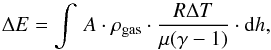 (4)where R = 8.31 J mol-1 K-1, μ = 1.3 g mol-1, and γ = 5/3 are the gas constant, the specific mass, and the adiabatic coefficient, respectively, while A denotes the area and h the height in which the value of ΔT is valid.
We used h = 500 km and integrated the density ρgas(z) in the HSRA model from z = 0 to 500 km for the photosphere and from 500 to 1000 km for the chromosphere. This yielded a total thermal energy in the EB at the time of the spectrograph observations of 8 × 10¹⁹ J in the photosphere and 3 × 10¹⁸ J in the chromosphere, respectively.
An order-of-magnitude estimate for the kinetic energy assuming a typical velocity of 1 km s-1 and 3 km s-1 in the photosphere and chromosphere results in 2 × 10¹⁹ J in the photosphere and 4 × 10¹⁸ J in the chromosphere, respectively. These numbers are approximately the same order of magnitude as the thermal and radiative energies.
5. Discussion
5.1. Doppler shifts associated with EBs
Socas-Navarro et al. (2006) found strongly redshifted chromospheric lines in EBs. These authors showed such redshifts in the Ca ii IR 849.8 nm line whose line core forms slightly deeper than the Ca ii IR 854 nm line and has a line-center opacity of about an order of magnitude less than the Ca ii IR 854 nm line (Linsky & Avrett 1970). We find a blueshift in simultaneous spectra of four chromospheric lines. The amount of Doppler shift is up to 40 km s-1 in the He i line and often exceeds 10 km s-1. We cannot necessarily attribute these blueshifts to an upflow since the observed region was far from disk center. A blueshift in the middle chromosphere is, however, consistent with the observed asymmetry of the Ca ii line profiles: the core of the line is blueshifted so it partially suppresses the violet peak while leaving the red peak unaffected. Matsumoto et al. (2008) found an upflow in the chromosphere and a downflow in the photosphere, while Bello González et al. (2013) and Vissers et al. (2013) reported up- and downflows associated with EBs.
5.2. Magnetic structure of the EB
From a timeseries of HMI magnetic flux maps (after conversion to the local reference frame), we see evidence of a magnetic flux cancellation (Sect. 2.6). Therefore, our results are in agreement with several authors who proposed a magnetic flux cancellation as the triggering mechanism of EBs (e.g., Nelson et al. 2013; Vissers et al. 2013; Bello González et al. 2013). The magnetic flux cancellation and the observed blueshifts compare well with the cartoon of Matsumoto et al. (2008) and Peter et al. (2014, their Fig. S7): a magnetic reconnection in the upper photosphere or around the temperature minimum results in an upflow in the chromospheric lines and a downflow in the photospheric lines. When the magnetic field lines are inclined and pointed toward the observer, the upflow can be seen as a horizontal blue- or redshift close to the limb. The photospheric redshifts are not as strong as chromospheric blueshifts since the density is several orders of magnitude higher in the photosphere so only a mild redshift can be expected in this scenario. In absence of a chromospheric magnetogram, a discussion of chromospheric reconnection is speculative. The temperature enhancement and the strong emission peaks are, however, signatures of an energy deposit in or energy transfer into the chromosphere. The HMI line forms in the middle of photosphere so we have only direct evidence for a photospheric flux cancellation. The magnetic reconnection scenario also has support from numerical modeling of resistive flux emergence in the solar surface (Archontis & Hood 2009). The magnetic field strength associated with the site of the EB in our data is comparable to the values reported by Socas-Navarro et al. (2006) and Bello González et al. (2013) who reported a field strength on the order of the equipartition value.
5.3. The radiative energy of the EB
The continuum contrast of the EB has a power-law dependency on the wavelength. The continuum intensity at the four longest wavelengths (630, 650, 854, and 1080 nm) were estimated from clear continuum windows in the vicinity of the spectral lines. Hence, they represent the temperature at the continuum forming region, even if the continuum at one micron forms at a few tens of kilometers below the one at the 650 nm wavelength range. In contrast, the pseudo-continuum at 397 nm is more representative of the middle or upper photosphere since there are no clear continuum windows in the UV part of the spectrum. The 170 nm continuum is mainly formed at the temperature minimum so these two data points in Fig. 7 are more an indicator of a temperature enhancement in the upper photosphere rather than the deep photosphere.
Fang et al. (2006) reported a temperature enhancement of 100−300 K when they took into account non-thermal effects while Georgoulis et al. (2002) found a temperature increase of 2000 K considering only thermal effects. We find an increase of about 130 K in the continuum forming layers and about 400 K at the height of the temperature minimum, at the low end of the values reported in literature, but also referring to slightly lower heights in the atmosphere. The temperature enhancement at the continuum level results in an excess emission integrated over all wavelengths (and the area of the EB) on the order of 1020 J, which is consistent with the results of Georgoulis et al. (2002) and Fang et al. (2006), while our EB is much more energetic than the ones reported by Nelson et al. (2013). The chromospheric radiative energy (Sect. 4.7) is on the order of 1017−1018 J, which is much smaller than the corresponding photospheric radiative energy. Although the EB in our data has distinct similarities to the cartoon of a hot explosive event observed by Peter et al. (2014), it does not show any trace of temperatures on the order of 105 K.
5.4. Increased line width associated with the EB
The EB profiles show a clear sign of enhanced line width in all chromospheric lines (Sect. 4). The increased line widths can be attributed to a larger temperature or a larger turbulence velocity, can be explained as a sign of twist (De Pontieu et al. 2014) or generally a signature of heating processes (Peter 2000). The estimated turbulence velocity in the EB is about twice as large as the turbulence velocity in a quiet chromosphere. It is not clear which fraction of the released energy goes into this non-thermal form instead of radiation. Attributing the observed line width solely to thermal broadening yields a temperature of a few 105 K. The mere existence of the He i 1083 nm and Hα lines in absorption suggests that the temperature in the middle and upper chromosphere does not increase to transition-region values of the order of 105 K. Vissers et al. (2013) did not find traces of EBs in the He ii 30.4 nm line or other EUV spectral lines, which is consistent with a typical temperature stratification in the middle and upper chromosphere resulting in an absorption profile for the He i 1083 nm line.
5.5. Formation height range of EBs
The bulk of the energy is released in the photosphere and only a small fraction is released in the chromosphere. The temperature excess increases with height in the photosphere. We find the He i line at 1083 nm in absorption, which is unlike its appearance in flare-like events (emission profile on disk). It indicates that most of the energy release happens in the lower chromosphere and deeper layers and does not modify the upper chromospheric part of the atmosphere significantly. At the same time the Si i line, whose core has contributions from the temperature minimum and above (Bard & Carlsson 2008), has a shallower line depth and the EB shows up clearly in its line-core map.
The helium line at 1083 nm might not be a good tracer of EBs because the EBs presumably happen in a lower atmospheric layer than the source region of the helium line. It is basically the same reason why the EBs are not seen as extreme bright sources in the very core of the Hα line. The helium line can, however, be used to reject the identification of an event as an EB. In case of flare events, this line on the solar disk shows an emission profile. This requires a substantial temperature rise in the middle and upper chromosphere, which does not seem to be the case for EBs. The core intensity of the Ca ii lines are larger than the average quiet Sun profile in contrast to the Hα and helium lines. The height range of the energy release should thus have some influence on the height range in which the core of the Ca ii lines form (~1 Mm).
We do not find the observed EB to be a purely photospheric phenomenon since it alters the lower chromospheric lines significantly while it does not create a temperature reversal in the photosphere. A substantial temperature rise in the photosphere results in spectral lines to be partially in emission. Stokes V profiles of such events are distinctly different from normal anti-symmetric profiles (Steiner 2000; Rezaei et al. 2007b). The simultaneous observation of the EB in multiple spectral lines presented in this paper strongly suggests that EBs have a minimum height range of a few pressure scale heights since they are seen from the deep photosphere in the continuum to the low chromosphere in the core of strong lines. Therefore, the site of the energy release should be higher than an altitude, which affects the Fe i 630 nm line pair, but low enough to modify the Si i 1082.7 nm line. This strongly suggests the temperature minimum as the probable location of the energy release, although the EB affects the temperature stratification over several pressure scale heights above and below the temperature minimum. The pressure scale height, kBT/μg, increases with height in the chromosphere since both the temperature increases and the ionization of hydrogen increases the number density of particles, which consequently decreases the mean molecular weight (μ). It has a value of about 100 km in the photosphere and increases above 200 km in the chromosphere. This means the EB spans a height range of less than 1000 km centered at about log τ = −4. This is consistent with strong emission peaks in Ca ii lines, a dark core in Hα line profile, large contrast in UV continuum, and a mild temperature enhancement in the deep photosphere.
We ran the CAlcium Inversion using a Spectral ARchive code (CAISAR, Beck et al. 2013b,c, 2015) over the region containing the EB for a visualization of the 3D structure. Figure 10 shows a 3D rendering of the corresponding region in the inversion results. The quantity that is displayed is the difference between the measured temperature in each pixel and the temperature stratification in a quiet Sun reference region, i.e., T(x,y,τ)− ⟨ TQS(τ) ⟩. The reason for selecting the relative instead of the absolute temperature was to extend the displayed volume down to the continuum-forming layers. The ray tracing selects the highest value along each ray to set the location and value of the displayed intensity, so the absolute photospheric temperature would otherwise dominate the 3D structure. The sunspot is towards the left in the image. The EB structure inside the blue square is seen to connect from the chromosphere down to the photosphere. It shows a slight lateral expansion in the low atmosphere and a somewhat more extended area in the chromosphere. The network region inside the white rectangle lacks the direct connection to the photosphere, i.e., there is no strong temperature enhancement in the low atmosphere in the network.
 |
Fig. 10 3D rendering of the EB in relative temperature (T− ⟨ TQS ⟩). The z-axis is in units of log τ500 nm. The location of the EB is indicated by a blue square. A patch of magnetic network is marked with a white rectangle. The panels at the top show maps of the temperature at a few levels in optical depth. |
Our results are in agreement with Payne (1993) and Harvey (1963) who characterized the formation height of EBs at the temperature minimum. The formation height range of the EB in our data is also consistent with Bello González et al. (2013), Matsumoto et al. (2008), and Fang et al. (2006) who attributed EBs to a height range around the temperature minimum. We do not find EBs to be purely photospheric phenomena, even if the driving forces could be located in the photosphere (Watanabe et al. 2011; Vissers et al. 2013). The Hα line profile of our EB is similar to the one reported by Vissers et al. (2013), but we note that the simultaneous Ca ii IR line profiles in our observations are significantly different from the ones they reported. This perhaps suggests that the two events are not quite the same and have a different formation height. We also note that the Ca ii IR line profile of an EB presented by Socas-Navarro et al. (2006) has almost no continuum enhancement compared to a quiet Sun profile, which is in contrast to the behavior of our profiles (bottom row, Fig. 9).
5.6. CaII H line: an ideal tracer of EBs
Ellerman bombs have been observed in the Ca ii H line by Hashimoto et al. (2010). We probe the diagnostic potential of the Ca ii H line profile to identify and study EBs. The shape of the wing and core of this line makes it an ideal tool with which to study EBs and distinguish them from network bright points, for example. Unlike the Hα line, which has contributions from a large height range in the atmosphere, the Ca ii H line has a formation height which gradually increases from the lower photosphere (the far wing) up to the middle and upper photosphere (the middle and inner wings) and to the lower chromosphere where the core of the line forms (Fig. 5 in Rezaei et al. 2008). In addition, it is easier to interpret the wing intensity maps of the Ca ii H line (Fig. 1) than the ones from the Hα line (Fig. 3).
6. Conclusion
We present for the first time a simultaneous observations of an EB in the Ca ii H, Ca ii IR 854 nm, Hα and He i 1083 nm lines. Our observations of an energetic event has similarities with the typical properties of an EB: it shows the blue and red wings of the Hα line in emission and has enhanced emission in the UV continuum. The magnetic flux cancellation in the EB area also exhibits a similarity to the general picture of an EB. We estimate the radiative energy content of the EB to be about 1020 J in the photosphere and about 1018 J in the chromosphere. We find the Ca ii H line to be an ideal tool with which to study EBs since the contribution function of different parts of the wing and core of the line span the whole photosphere up to the lower chromosphere. The He i line at 1083 nm, on the other hand, seems unsuitable for the detection of EBs, but could serve to reject false identifications by showing emission profiles.
Ellerman bombs release their energy at a height span of several pressure scale heights around the temperature minimum. They are not located at the middle and upper chromosphere, nor can they be placed deep in the photosphere.
Acknowledgments
We thank Andreas Lagg for making the HeLIx+ code available to us. We acknowledge Nazaret Bello González for helpful suggestions. The POLIS instrument has been developed by the Kiepenheuer-Institut in cooperation with the High Altitude Observatory (Boulder, USA). The German VTT is operated by the Kiepenheuer-Institut für Sonnenphysik at the Spanish Observatorio del Teide of the Instituto de Astrofísica de Canarias (IAC). R.R. acknowledges financial support by the DFG grant RE 3282/1-1.
References
- Archontis, V., & Hood, A. W. 2009, A&A, 508, 1469 [NASA ADS] [CrossRef] [EDP Sciences] [Google Scholar]
- Balthasar, H., Thiele, U., & Woehl, H. 1982, A&A, 114, 357 [NASA ADS] [Google Scholar]
- Bard, S., & Carlsson, M. 2008, ApJ, 682, 1376 [NASA ADS] [CrossRef] [Google Scholar]
- Beck, C. 2006, Ph.D. Thesis, Albert-Ludwigs-University, Freiburg [Google Scholar]
- Beck, C. 2008, A&A, 480, 825 [NASA ADS] [CrossRef] [EDP Sciences] [Google Scholar]
- Beck, C., & Rezaei, R. 2012, in Second ATST-EAST Meeting: Magnetic Fields from the Photosphere to the Corona., eds. T. R. Rimmele, A. Tritschler, F. Wöger, et al., ASP Conf. Ser., 463, 257 [Google Scholar]
- Beck, C., Schlichenmaier, R., Collados, M., Bellot Rubio, L., & Kentischer, T. 2005a, A&A, 443, 1047 [NASA ADS] [CrossRef] [EDP Sciences] [Google Scholar]
- Beck, C., Schmidt, W., Kentischer, T., & Elmore, D. 2005b, A&A, 437, 1159 [NASA ADS] [CrossRef] [EDP Sciences] [Google Scholar]
- Beck, C., Mikurda, K., Bellot Rubio, L. R., Kentischer, T., & Collados, M. 2007, in Modern solar facilities – advanced solar science, eds. F. Kneer, K. G. Puschmann, & A. D. Wittmann, 55 [Google Scholar]
- Beck, C., Schmidt, W., Rezaei, R., & Rammacher, W. 2008, A&A, 479, 213 [NASA ADS] [CrossRef] [EDP Sciences] [Google Scholar]
- Beck, C., Rezaei, R., & Fabbian, D. 2011, A&A, 535, A129 [NASA ADS] [CrossRef] [EDP Sciences] [Google Scholar]
- Beck, C., Fabbian, D., Moreno-Insertis, F., Puschmann, K. G., & Rezaei, R. 2013a, A&A, 557, A109 [NASA ADS] [CrossRef] [EDP Sciences] [Google Scholar]
- Beck, C., Rezaei, R., & Puschmann, K. G. 2013b, A&A, 549, A24 [NASA ADS] [CrossRef] [EDP Sciences] [Google Scholar]
- Beck, C., Rezaei, R., & Puschmann, K. G. 2013c, A&A, 553, A73 [NASA ADS] [EDP Sciences] [Google Scholar]
- Beck, C., Choudhary, D. P., Rezaei, R., & Louis, R. E. 2015, ApJ, 798, 100 [NASA ADS] [CrossRef] [Google Scholar]
- Bello González, N., Danilovic, S., & Kneer, F. 2013, A&A, 557, A102 [NASA ADS] [CrossRef] [EDP Sciences] [Google Scholar]
- Bellot Rubio, L. R. 2003, Inversion of Stokes profiles with SIR (Freiburg: Kiepenheuer Institut für Sonnenphysik) [Google Scholar]
- Berkefeld, T., Soltau, D., Schmidt, D., & von der Lühe, O. 2010, Appl. Opt., 49, G155 [CrossRef] [Google Scholar]
- Berlicki, A., Heinzel, P., & Avrett, E. H. 2010, Mem. Soc. Astron. Italiana, 81, 646 [Google Scholar]
- Böhm-Vitense, E. 1989, Introduction to stellar astrophysics, Vol. 2, Stellar atmospheres (CUP) [Google Scholar]
- Borrero, J. M., Tomczyk, S., Norton, A., et al. 2007, Sol. Phys., 240, 177 [NASA ADS] [CrossRef] [Google Scholar]
- Borrero, J. M., Tomczyk, S., Kubo, M., et al. 2011, Sol. Phys., 273, 267 [Google Scholar]
- Borrero, J. M., Lites, B. W., Lagg, A., Rezaei, R., & Rempel, M. 2014, A&A, 572, A54 [NASA ADS] [CrossRef] [EDP Sciences] [Google Scholar]
- Bruzek, A. 1972, Sol. Phys., 26, 94 [NASA ADS] [CrossRef] [Google Scholar]
- Collados, M., Lagg, A., Díaz Garcí A, J. J., et al. 2007, in The Physics of Chromospheric Plasmas, eds. P. Heinzel, I. Dorotovič, & R. J. Rutten, ASP Conf. Ser., 368, 611 [Google Scholar]
- Cram, L. E., & Damé, L. 1983, ApJ, 272, 355 [NASA ADS] [CrossRef] [Google Scholar]
- Dara, H. C., Alissandrakis, C. E., Zachariadis, T. G., & Georgakilas, A. A. 1997, A&A, 322, 653 [NASA ADS] [Google Scholar]
- De Pontieu, B., Rouppe van der Voort, L., McIntosh, S. W., et al. 2014, Science, 346, 315 [Google Scholar]
- Ellerman, F. 1917, ApJ, 46, 298 [NASA ADS] [CrossRef] [Google Scholar]
- Elmore, D. F., Lites, B. W., Tomczyk, S., et al. 1992, in SPIE Conf. Ser. 1746, eds. D. H. Goldstein, & R. A. Chipman, 22 [Google Scholar]
- Fang, C., Tang, Y. H., Xu, Z., Ding, M. D., & Chen, P. F. 2006, ApJ, 643, 1325 [NASA ADS] [CrossRef] [Google Scholar]
- Felipe, T., Khomenko, E., Collados, M., & Beck, C. 2010, ApJ, 722, 131 [NASA ADS] [CrossRef] [Google Scholar]
- Filippenko, A. V. 1982, PASP, 94, 715 [NASA ADS] [CrossRef] [Google Scholar]
- Georgoulis, M. K., Rust, D. M., Bernasconi, P. N., & Schmieder, B. 2002, ApJ, 575, 506 [NASA ADS] [CrossRef] [Google Scholar]
- Harvey, J. W. 1963, The Observatory, 83, 37 [NASA ADS] [Google Scholar]
- Harvey, K., & Harvey, J. 1973, Sol. Phys., 28, 61 [NASA ADS] [CrossRef] [Google Scholar]
- Hashimoto, Y., Kitai, R., Ichimoto, K., et al. 2010, PASJ, 62, 879 [NASA ADS] [Google Scholar]
- Hong, J., Ding, M. D., Li, Y., Fang, C., & Cao, W. 2014, ApJ, 792, 13 [NASA ADS] [CrossRef] [Google Scholar]
- Judge, P. 2006, in Solar MHD Theory and Observations: A High Spatial Resolution Perspective, eds. J. Leibacher, R. F. Stein, & H. Uitenbroek, ASP Conf. Ser., 354, 259 [Google Scholar]
- Kiess, C., Rezaei, R., & Schmidt, W. 2014, A&A, 565, A52 [NASA ADS] [CrossRef] [EDP Sciences] [Google Scholar]
- Kitai, R., & Muller, R. 1984, Sol. Phys., 90, 303 [NASA ADS] [CrossRef] [Google Scholar]
- Kneer, F. 2010, Mem. Soc. Astron. It., 81, 604 [NASA ADS] [Google Scholar]
- Kneer, F., & Mattig, W. 1978, A&A, 65, 17 [NASA ADS] [Google Scholar]
- Kucera, A., Beck, C., Gömöry, P., et al. 2008, 12th European Solar Physics Meeting, Freiburg, Germany, 12, 2 [Google Scholar]
- Kurokawa, H., Kawaguchi, I., Funakoshi, Y., & Nakai, Y. 1982, Sol. Phys., 79, 77 [NASA ADS] [CrossRef] [Google Scholar]
- Kurucz, R. L., Furenlid, I., Brault, J., & Testerman, L. 1984, Solar Flux Atlas From 296 nm to 1300 nm (National Solar Observatory) [Google Scholar]
- Lagg, A. 2007, Adv. Space Res., 39, 1734 [Google Scholar]
- Lagg, A., Woch, J., Krupp, N., & Solanki, S. K. 2004, A&A, 414, 1109 [NASA ADS] [CrossRef] [EDP Sciences] [Google Scholar]
- Lemen, J. R., Title, A. M., Akin, D. J., et al. 2012, Sol. Phys., 275, 17 [NASA ADS] [CrossRef] [Google Scholar]
- Linsky, J. L., & Avrett, E. H. 1970, PASP, 82, 169 [NASA ADS] [CrossRef] [Google Scholar]
- Lites, B. W., & Skumanich, A. 1982, ApJS, 49, 293 [NASA ADS] [CrossRef] [Google Scholar]
- Lites, B. W., Rutten, R. J., & Kalkofen, W. 1993, ApJ, 414, 345 [NASA ADS] [CrossRef] [Google Scholar]
- Lites, B. W., Low, B. C., Martinez Pillet, V., et al. 1995, ApJ, 446, 877 [NASA ADS] [CrossRef] [Google Scholar]
- Martínez Pillet, V., Collados, M., Sánchez Almeida, J., et al. 1999, in High Resolution Solar Physics: Theory, Observations, and Techniques, ASP Conf. Ser., 183, 264 [NASA ADS] [Google Scholar]
- Matsumoto, T., Kitai, R., Shibata, K., et al. 2008, PASJ, 60, 95 [NASA ADS] [Google Scholar]
- McMath, R. R., Mohler, O. C., & Dodson, H. W. 1960, PNAS, 46, 165 [Google Scholar]
- Metcalf, T. R. 1994, Sol. Phys., 155, 235 [Google Scholar]
- Metcalf, T. R., Leka, K. D., Barnes, G., et al. 2006, Sol. Phys., 237, 267 [Google Scholar]
- Neckel, H., & Labs, D. 1984, Sol. Phys., 90, 205 [NASA ADS] [CrossRef] [Google Scholar]
- Neckel, H., & Labs, D. 1994, Sol. Phys., 153, 91 [NASA ADS] [CrossRef] [Google Scholar]
- Nelson, C. J., Shelyag, S., Mathioudakis, M., et al. 2013, ApJ, 779, 125 [NASA ADS] [CrossRef] [Google Scholar]
- Nindos, A., & Zirin, H. 1998, Sol. Phys., 182, 381 [NASA ADS] [CrossRef] [Google Scholar]
- Pariat, E., Aulanier, G., Schmieder, B., et al. 2004, ApJ, 614, 1099 [Google Scholar]
- Pariat, E., Schmieder, B., Berlicki, A., et al. 2007, A&A, 473, 279 [NASA ADS] [CrossRef] [EDP Sciences] [Google Scholar]
- Parker, E. N. 1988, ApJ, 330, 474 [Google Scholar]
- Payne, T. E. W. 1993, Ph.D. Thesis, New Mexico State University [Google Scholar]
- Pesnell, W. D., Thompson, B. J., & Chamberlin, P. C. 2012, Sol. Phys., 275, 3 [NASA ADS] [CrossRef] [Google Scholar]
- Peter, H. 2000, A&A, 360, 761 [NASA ADS] [Google Scholar]
- Peter, H., Tian, H., Curdt, W., et al. 2014, Science, 346, C315 [NASA ADS] [CrossRef] [Google Scholar]
- Qiu, J., Ding, M. D., Wang, H., Denker, C., & Goode, P. R. 2000, ApJ, 544, L157 [NASA ADS] [CrossRef] [Google Scholar]
- Reardon, K. P. 2006, Sol. Phys., 239, 503 [NASA ADS] [CrossRef] [Google Scholar]
- Rezaei, R. 2008, Ph.D. Thesis, Albert-Ludwigs University, Freiburg [Google Scholar]
- Rezaei, R., Schlichenmaier, R., Beck, C., & Bellot Rubio, L. R. 2006, A&A, 454, 975 [NASA ADS] [CrossRef] [EDP Sciences] [Google Scholar]
- Rezaei, R., Schlichenmaier, R., Beck, C., Bruls, J., & Schmidt, W. 2007a, A&A, 466, 1131 [NASA ADS] [CrossRef] [EDP Sciences] [Google Scholar]
- Rezaei, R., Schlichenmaier, R., Schmidt, W., & Steiner, O. 2007b, A&A, 469, L9 [NASA ADS] [CrossRef] [EDP Sciences] [Google Scholar]
- Rezaei, R., Bruls, J. H. M. J., Schmidt, W., et al. 2008, A&A, 484, 503 [NASA ADS] [CrossRef] [EDP Sciences] [Google Scholar]
- Rezaei, R., Bello González, N., & Schlichenmaier, R. 2012, A&A, 537, A19 [NASA ADS] [CrossRef] [EDP Sciences] [Google Scholar]
- Roy, J.-R., & Leparskas, H. 1973, Sol. Phys., 30, 449 [NASA ADS] [CrossRef] [Google Scholar]
- Ruiz Cobo, B., & del Toro Iniesta, J. C. 1992, ApJ, 398, 375 [NASA ADS] [CrossRef] [Google Scholar]
- Rutten, R. J. 2003, Radiative Transfer in Stellar Atmosphere (Sterrekundig Instituut Utrecht, Institute of Theoretical Astrophysics, Oslo) [Google Scholar]
- Rutten, R. J., Vissers, G. J. M., Rouppe van der Voort, L. H. M., Sütterlin, P., & Vitas, N. 2013, J. Phys. Conf. Ser., 440, 012007 [NASA ADS] [CrossRef] [Google Scholar]
- Scherrer, P. H., Schou, J., Bush, R. I., et al. 2012, Sol. Phys., 275, 207 [Google Scholar]
- Schlichenmaier, R., & Collados, M. 2002, A&A, 381, 668 [NASA ADS] [CrossRef] [EDP Sciences] [Google Scholar]
- Schmidt, W., Beck, C., Kentischer, T., Elmore, D., & Lites, B. 2003, Astron. Nachr., 324, 300 [NASA ADS] [CrossRef] [Google Scholar]
- Schou, J., Scherrer, P. H., Bush, R. I., et al. 2012, Sol. Phys., 275, 229 [Google Scholar]
- Schröter, E. H., Soltau, D., & Wiehr, E. 1985, Vist. Astron., 28, 519 [NASA ADS] [CrossRef] [Google Scholar]
- Severny, A. 1957, Izv. Krymskoi. Ast. Obs., 17, 129 [Google Scholar]
- Severny, A. B. 1968, in Mass Motions in Solar Flares and Related Phenomena, ed. Y. Oehman, 71 [Google Scholar]
- Socas-Navarro, H., Martínez Pillet, V., Elmore, D., et al. 2006, Sol. Phys., 235, 75 [NASA ADS] [CrossRef] [Google Scholar]
- Steiner, O. 2000, Sol. Phys., 196, 245 [NASA ADS] [CrossRef] [Google Scholar]
- Stellmacher, G., & Wiehr, E. 1991, A&A, 251, 675 [NASA ADS] [Google Scholar]
- Stix, M. 2002, The Sun: An Introduction, 2nd edn. (Berlin: Springer-Verlag) [Google Scholar]
- Tandberg-Hanssen, E. 1960, Astrophys. Norvegica, 6, 161 [Google Scholar]
- Tomczyk, S., Elmore, D. F., Lites, B. W., et al. 1992, BAAS, 24, 814 [NASA ADS] [Google Scholar]
- Vernazza, J. E., Avrett, E. H., & Loeser, R. 1981, ApJS, 45, 635 [NASA ADS] [CrossRef] [Google Scholar]
- Vissers, G. J. M., Rouppe van der Voort, L. H. M., & Rutten, R. J. 2013, ApJ, 774, 32 [NASA ADS] [CrossRef] [Google Scholar]
- von der Lühe, O., Soltau, D., Berkefeld, T., & Schelenz, T. 2003, in Innovative Telescopes and Instrumentation for Solar Astrophysics, eds. S. L. Keil, & S. V. Avakyan, SPIE, 4853, 187 [Google Scholar]
- Watanabe, H., Kitai, R., Okamoto, K., et al. 2008, ApJ, 684, 736 [NASA ADS] [CrossRef] [Google Scholar]
- Watanabe, H., Vissers, G., Kitai, R., Rouppe van der Voort, L., & Rutten, R. J. 2011, ApJ, 736, 71 [NASA ADS] [CrossRef] [Google Scholar]
All Tables
All Figures
|
Fig. 1 Overview maps of the observed area. Top row, left to right: the intensity of the Ca ii H pseudo-continuum in the far blue wing, the outer and inner wing intensities, and the line-core intensity (H3). Middle row: the intensity of the Ca ii IR continuum, the monochromatic intensity at −10 and +5 pm from the line core, and the line-core intensity. Bottom row: the Si i continuum intensity, the polarization degree from the POLIS Fe i 630 nm data, the Si i line-core intensity, and the He i line-core intensity. The intensity maps are normalized to the nearby continuum intensity of the average quiet Sun. The contour and circle outline a magnetic field strength of 700 G and the location of the EB, respectively. The arrow marks the direction of disk center. |
| In the text | |
|
Fig. 2 AIA data. Top row: filtergrams at 160 and 170 nm co-temporal with the profiles shown in Fig. 9. For a description of the contour and circle, see Fig. 1. Bottom panel: temporal variation of the intensity of the EB in AIA 160 and 170 nm images. The vertical lines mark the time span of the VTT observations. The red line marks the time at which the the slit passed across the EB. |
| In the text | |
|
Fig. 3 The Ellerman bomb in the Hα line. All values are in units of the continuum intensity of the average quiet Sun profile at 656 nm. For a description of the contour and circle, see Fig. 1. |
| In the text | |
|
Fig. 4 Velocity maps. Top, left to right: the absolute line-core velocity of Fe i 630.25 nm line, line-core velocity of Si i 1082.7 nm line retrieved via SIR inversion, and Ca ii H center-of-gravity velocity. Bottom, left to right: Hα, Ca ii IR line-core, and He i 1083 nm line-core velocity obtained by the HeLIx+ inversion. The center-of-gravity velocity of Ca ii H line was calculated for a spectral range of 100 pm around the line core. All velocities are in km s-1. |
| In the text | |
|
Fig. 5 Left to right: photospheric magnetic field strength from SIR inversion (G), chromospheric magnetic field strength from HeLIx+ inversion (G), and the LRF inclination maps of HMI data at 07:00 and 08:12 (deg). For a description of the contour and circle, see Fig. 1. |
| In the text | |
|
Fig. 6 Magnetic field inclination (top) and flux (bottom) in the local reference frame from HMI data with 12-min cadence. Time increases from left to right between 7:00 and 8:36. The contour, circle, and coordinates are as in the full maps (Figs. 1, 3–5). The yellow patch seen in the center of the circle at left in the flux maps disappears gradually. Inclination is in degrees and flux in G. |
| In the text | |
|
Fig. 7 The log–log plot of the continuum contrast vs. wavelength. The 160 nm data, which has contamination from transition region emission line, was not used for the linear fit (solid line). Numbers next to each data point show the wavelength in nm. The error bar of Ca ii IR continuum is larger mainly due to uncorrected fringes. |
| In the text | |
|
Fig. 8 Line profiles. Each row shows one spectral band. The three panels in each row show individual EB profiles (EB-1..7) along with a neighboring profile (EB-n) and the average quiet Sun profile. From top to bottom: the Fe i line pair at 630 nm, the He i 1083 nm and Si i 1082.7 nm Stokes I profile, and the corresponding Stokes V profile. The profiles are located inside the circle in Fig. 1 which outlines the EB. |
| In the text | |
|
Fig. 9 Similar to Fig. 8 but for chromospheric lines. From top to bottom: the Hα line profile, the Ca ii H line profile, and the Ca ii IR intensity profile. We note the enhanced amplitude and width of the red emission peak pf Ca ii lines in the EB compared to the average quiet Sun profiles. The blueshift is clearly seen in the Hα line profile. |
| In the text | |
|
Fig. 10 3D rendering of the EB in relative temperature (T− ⟨ TQS ⟩). The z-axis is in units of log τ500 nm. The location of the EB is indicated by a blue square. A patch of magnetic network is marked with a white rectangle. The panels at the top show maps of the temperature at a few levels in optical depth. |
| In the text | |
Current usage metrics show cumulative count of Article Views (full-text article views including HTML views, PDF and ePub downloads, according to the available data) and Abstracts Views on Vision4Press platform.
Data correspond to usage on the plateform after 2015. The current usage metrics is available 48-96 hours after online publication and is updated daily on week days.
Initial download of the metrics may take a while.