| Issue |
A&A
Volume 582, October 2015
|
|
|---|---|---|
| Article Number | A47 | |
| Number of page(s) | 8 | |
| Section | Interstellar and circumstellar matter | |
| DOI | https://doi.org/10.1051/0004-6361/201526000 | |
| Published online | 05 October 2015 | |
3D hydrodynamic simulations of the Galactic supernova remnant CTB 109
1 Zentrum für Astronomie und Astrophysik, TU Berlin, Hardenbergstraße 36, 10623 Berlin, Germany
e-mail: This email address is being protected from spambots. You need JavaScript enabled to view it.
2 Institut für Astronomie und Astrophysik, Universität Tübingen, Sand 1, 72076 Tübingen, Germany
Received: 2 March 2015
Accepted: 22 August 2015
Abstract
Context. Using detailed 3D hydrodynamic simulations we study the nature of the Galactic supernova remnant (SNR) CTB 109 (G109.1-1.0), which is well known for its semicircular shape and a bright diffuse X-ray emission feature inside the SNR.
Aims. Our model has been designed to explain the observed morphology, with a special emphasis on the bright emission feature inside the SNR. Moreover, we determine the age of the remnant and compare our findings with X-ray observations. With CTB 109 we test a new method of detailed numerical simulations of diffuse young objects, using realistic initial conditions derived directly from observations.
Methods. We performed numerical 3D simulations with the RAMSES code. The initial density structure has been directly taken from 12CO emission data, adding an additional dense cloud, which, when it is shocked, causes the bright emission feature.
Results. From parameter studies we obtained the position (ℓ,b) = (109.1545°,−1.0078°) for an elliptical cloud with ncloud = 25 cm-3 based on the preshock density from Chandra data and a maximum diameter of 4.54 pc, whose encounter with the supernova (SN) shock wave generates the bright X-ray emission inside the SNR. The calculated age of the remnant is about 11 000 yr according to our simulations. In addition, we can also determine the most probable site of the SN explosion.
Conclusions. Hydrodynamic simulations can reproduce the morphology and the observed size of the SNR CTB 109 remarkably well. Moreover, the simulations show that it is very plausible that the bright X-ray emission inside the SNR is the result of an elliptical dense cloud shocked by the SN explosion wave. We show that numerical simulations using observational data for an initial model can produce meaningful results.
Key words: ISM: supernova remnants / evolution / shock waves / hydrodynamics / methods: numerical
© ESO, 2015
1. Introduction
In astronomy, complex morphologies of diffuse objects with filamentary or wispy structures, for example, are often difficult to explain because the ambient medium is very inhomogeneous, and/or dynamical changes in the flow (e.g. shock waves) modify the emission or absorption processes significantly. If one would like to know if a certain feature is due to hydrodynamic interactions, a numerical simulation could help to clarify the conditions under which it has originated. A typical case is the X-ray observation of supernova remnants (SNRs). Here we present a method that exploits the fact that the molecular environment of an SNR has a high inertia, and does not evolve much within a typical early Sedov-Taylor phase time scale of the order of 104 yr. Therefore, the initial background model, if taken from 12CO observations, can be scanned identically into a computational grid. However, the observational background is a projection onto the plane of the sky and has to be extended to three dimensions. Nevertheless, such an initial model represents the real situation much better than previous simplifications, such as a homogeneous background. Density inhomogeneities lead to mass loading of the flow and hence to a quite different dynamical and thermal history of the plasma.
 |
Fig. 1 Left: 1420-MHz radio continuum image of CTB 109 (Kothes et al. 2002) from the Canadian Galactic Plane Survey (CGPS, Taylor et al. 2003). Right: intensity map (0.3−4.0 keV) of CTB 109 in false colour from the XMM-Newton EPIC data (Sasaki et al. 2004). The very bright point source is the AXP 1E 2259+586 and the diffuse emission at RA = 2302, Dec =+ 58°55′ (J2000.0) with an extent of ~7′ is the Lobe. Chandra’s field of view is marked as a white rectangle. |
The Galactic SNR CTB 109 (G109.1-1.0) associated with the anomalous X-ray pulsar (AXP) 1E 2259+586 was first detected in X-rays by the satellite mission Einstein in 1980 (Gregory & Fahlman 1980) and has been regularly observed ever since.
Radio observations at λ49 cm (Hughes et al. 1981, 1984), λ21 cm (Hughes et al. 1984; Braun & Strom 1986), λ4.6 cm (Hughes et al. 1984), and at 2.7 GHz (Downes 1983) show a morphology that corresponds well to that observed in X-rays with the satellite Einstein. However, no radio emission has been detected from the AXP. The analysis of CO observations (Tatematsu et al. 1987; Kothes et al. 2002; Taylor et al. 2003) has revealed that the western part of the SNR has encountered a giant molecular cloud (GMC) complex, resulting in a semicircular shape of the remnant. Moreover, in radio a double-shell structure can be seen (see Fig. 1 (left)). After the first detection with Einstein, CTB 109 was observed in X-rays with ROSAT PSPC and BBXT (Rho & Petre 1993, 1997), BeppoSAX (Parmar et al. 1998, 1999), and ASCA (Rho et al. 1998). Partial X-ray shells were identified in the east, south, and north surrounding the AXP, but no shell structure was found in the west owing to the GMC. Moreover, an X-ray bright interior region called the X-ray lobe was identified in CTB 109. Higher resolution studies in X-rays were performed by XMM-Newton (Sasaki et al. 2004), Chandra (Sasaki et al. 2006, 2013), and Suzaku (Nakano et al. 2015) to investigate the remnant in more detail. The γ-ray observations by Fermi-LAT (Castro et al. 2012) complement the multi-wavelength view of CTB 109.
The determination of the distance to an SNR is quite challenging. Recent measurements show that the distance to CTB 109 lies between 3 and 4 kpc (Kothes et al. 2002; Tian et al. 2010); the latest value is 3.2 ± 0.2 kpc (Kothes & Foster 2012). It is even more difficult to determine the proper motion of the associated anomalous X-ray pulsar. The analysis by Kaplan et al. (2009) yields (μα,μδ) = (−11 ± 20 mas yr-1,−35 ± 20 mas yr-1), which is larger than the values (μα,μδ) = (−6.4 ± 0.6 mas yr-1,−2.3 ± 0.6 mas yr-1) from Tendulkar et al. (2013) where the uncertainties are much smaller.
The X-ray observations with XMM-Newton (Sasaki et al. 2004) show two prominent features of the SNR. Firstly, it has a semicircular shape due to a giant molecular cloud (GMC) complex in the west and secondly, a bright diffuse emission region, which is known as the “Lobe”, can be seen (see Fig. 1 (right)). It was discovered by Tatematsu et al. (1987) that the GMC complex extends even to the front of the remnant. Consequently, the Lobe could simply result from a projection effect, i.e. the result of a “hole”, a region with little or no absorption for X-rays, in the GMC. Alternatively, this particular emission feature could be caused by a shock heated cloud fragment, yielding bright X-ray emission.
In Sasaki et al. (2006) the velocity profiles (from high-resolution 12CO data from the Five College Radio Astronomy Observatory) and Chandra data of three molecular clouds around the Lobe were analysed. One of the clouds partly overlap with the Lobe. In various parts of this cloud the 12CO velocity profile fits very well with a Gaussian. However, where the Lobe and the cloud overlap, the velocity profile deviates from being Gaussian and has an additional component towards higher negative velocities. This indicates an additional acceleration in this part of the cloud, e.g. by a supernova (SN) blast wave. Moreover, the molecular hydrogen column densities in this region are relatively high, while the foreground absorption in X-rays is lower than in other parts. This could also be explained by an interaction between a SN shock wave and a dense cloud. Consequently, these results give new evidence for the hypothesis that the Lobe is the result of a shocked dense cloud.
In this work we will verify this hypothesis by 3D hydrodynamic simulations of the SNR. For this purpose an initial density distribution, which is based on 12CO observations, is supplemented with an additional cloud. By varying the properties of this homogeneous cloud, i.e. its position, size, shape, orientation, and density, the observed morphology and the X-ray emission of CTB 109 can be reproduced very well.
2. Hydrodynamic simulations
2.1. Previous modelling efforts
2.1.1. Analytic models
The first efforts to model the evolution of CTB 109 were made by Hughes et al. (1981) who used the Sedov-Taylor solution (Sedov 1959; Taylor 1946, 1950) to estimate the age of the remnant. For a homogeneous spherically symmetric medium they obtained an age of 17 000 yr from the Einstein data. In 1991, when the semicircular morphology of the SNR was already known, Ni et al. (1990) used the same method only for the eastern part and obtained an age of 13 000 yr. For the western part they used the analytic solution for the pressure-driven snowplow phase (e.g. McKee & Ostriker 1977) to describe the propagation of the blast wave into the GMC. In Sasaki et al. (2004, 2013), observational data again only from the eastern part obtained with XMM-Newton and Chandra, respectively, were used to estimate the age of CTB 109 with the Sedov-Taylor solution. For the XMM-Newton data an age of ~9400 ± 1000 yr was derived while the Chandra data yielded an age of 14 000 ± 2000 yr. The same age estimation was obtained from Suzaku data by Nakano et al. (2015) when applying the Sedov-Taylor similarity solution. For the alternative assumption that the SNR is in the snowplow phase, they derive 10 000 yr as an age.
2.1.2. Hydrodynamic models
A first model of CTB 109 which is not based on a similarity solution is described by Wang et al. (1992). They used the thin shell approximation (Kompaneets 1960) to describe the hydrodynamics of the semicircular SNR. Therefore, they divided the system into a uniform interstellar medium in the east, in which a SN explodes, and a uniform dense molecular cloud in the west. The interface between the two media is planar and 2 pc away from the explosion centre. Around the explosion centre, the domain is divided into 100 rings for which the spherically symmetric hydrodynamic equations are solved, using a numerical code by Mac Low & McCray (1988) and Chu & Mac Low (1990). This simulation reproduces the semicircular morphology of CTB 109 quite well. For an initial energy of E0 = 3.6 × 1050 erg, an ambient ISM density of n0 = 0.13 cm-3, and a cloud density of ncloud = 36 cm-3 the shape of the simulated remnant matches the Einstein data after 13 000 yr.
In 2012 a sophisticated broadband study of CTB 109 was carried out by Castro et al. (2012). Their spherically symmetric model includes hydrodynamics, efficient cosmic-ray acceleration, non-thermal emission, and a self-consistent calculation of the X-ray thermal emission as described in detail by Ellison et al. (2007) and Patnaude et al. (2009). The evolution of the remnant with a power-law ejecta density profile is considered in a circumstellar medium (CSM) with uniform density. The main focus of their study is to reproduce the broadband radio, X-ray, and γ-ray spectrum of CTB 109. For two distinct parameter sets, describing the hadronic and leptonic components for the γ-ray flux reasonable fits were found. However, because the X-ray spectrum of the SNR is dominated by thermal emission, a scenario where both relativistic leptons and hadrons contribute to the emission is more likely. Taking this into account, they found a better fit to the observations, which gives an ambient CSM density of n0 = 0.5 cm-3 and an age of 11 000 yr for a distance to CTB 109 of 2.8 kpc.
2.1.3. Comparison with our model
Previous models of CTB 109 concentrated mainly on the estimation of the age (Hughes et al. 1981; Ni et al. 1990; Sasaki et al. 2004, 2013; Nakano et al. 2015), only Wang et al. (1992) aimed at reproducing of a simple semicircular morphology, and Castro et al. (2012) focused on the broadband emission. For this purpose, simple spherically symmetric hydrodynamic models are sufficient. However, aiming at a detailed simulation of the observed complex morphology, which differs from being purely semicircular, no spherically symmetric model can be used. Therefore, we use a highly inhomogeneous ambient density structure from observation, which includes the GMC in the west. This would favour a 2D simulation. However, developing turbulent structures and the occurring instabilities, which yield the break-up of the SN shell, are entirely different in 2D than in 3D (Elmegreen & Scalo 2004; Kane et al. 2000). While turbulence in nature is an inherently 3D process, one might think of turbulent flows that are approximately 2D, in the sense that large scale coupling of eddies clearly exceeds the extension in one particular dimension. However, the physical properties between 2D and 3D turbulence are vastly different, so that sacrificing one dimension for a higher spatial resolution might lead to erroneous results. In contrast to 3D, as has been noted by Batchelor (1969) and Kraichnan (1967), due to the conservation of vorticity in 2D (in the incompressible, inviscid case without external forcing), the energy cascade is reversed, i.e. from small to large scales, while enstrophy flows in the opposite direction (double-cascade). In particular, we want to model the bright X-ray emission feature inside the SNR for the first time as a result of a shocked dense cloud. For this reason an additional cloud is added to the initial density structure, precluding again a 1D or 2D model.
To estimate the age of CTB 109 and to reproduce its semicircular morphology, a complex 3D model is not necessary and make it even more difficult to study many different parameter sets. However, our simulations complement the previous studies on CTB 109 by analysing the effect of an inhomogeneous medium on the evolution of the SNR and by simulating the bright X-ray emission region inside the SNR by a shocked dense cloud. These aspects could not be studied with their spherically symmetric models.
The details of the thermal and non-thermal emission of the SNR, which are modelled in detail by Castro et al. (2012), are beyond the scope of our study. We investigate in detail the X-ray emissivity to compare our finding with the X-ray observations. In forthcoming studies, spectral modelling will also be considered.
2.2. Numerical details of our studies
Reproducing observations by numerical simulations represents an inverse problem, which, as it is well-known, does not always possess a unique solution or even a solution at all. We simplify the problem by assuming that the background medium, due to its high inertia, has not changed significantly during the short evolution of the SNR, or in other words, we use the present ambient medium as the initial model.
The numerical simulations were performed with the RAMSES code (Teyssier 2002). The code works on 1D, 2D, or 3D unstructured Cartesian grids and solves the discretised Euler equations in their conservative form with a second-order Godunov scheme for a perfect gas (Piecewise Linear Method). In particular, the MUSCL scheme (Monotonic Upstream-Centred Scheme for Conservation Law, van Leer 1976, 1979) with the HLLC Riemann solver (Toro et al. 1994) was used where the MinMod slope limiter (Roe 1981) is employed to obtain a total variation diminishing discretisation scheme (Harten 1983). A 58 pc cube, which comprises the SNR and the GMC, is initially uniformly discretised into 1283 cells, hence the initial resolution of the grid is 0.45 pc. Based on a refinement strategy, which refines cells adaptively if steep pressure gradients occur, the grid is refined during the evolution of the SNR. The finest resolved structures due to the adaptive mesh refinement (AMR) have a size of 0.1 pc.
Given that the age of the SNR is ~104 yr, we can omit its free-expansion phase in the simulation because the duration of this phase is only ≲1000 yr. The reverse shock must have formed and already reached the centre of the SNR heating the ejecta. Therefore, the Sedov-Taylor similarity solution can be applied. Even though the ejecta might have had inhomogeneities like a Si clump as suggested by Sasaki et al. (2013), such clumps should have no significant effect on the overall evolution of the forward shock of the SNR expanding into the ISM. Furthermore, the end of the free-expansion phase is characterised by the fact that the mass of the swept-up interstellar material exceeds the mass of the ejecta, i.e. we can neglect the ejecta in our simulations. Consequently, the SN explosion can be modelled by a point-explosion, i.e. the pressure p0 in the 23 cells at the explosion centre is given as p0 = 3 (γ−1) E0/ (4 π (Δx)3) with Δx = 0.45 pc which yields the expanding remnant. As long as the dynamical time t is smaller than the cooling time 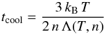 (1)(e.g. Spitzer 1978) with number density n, temperature T, cooling function Λ, and Boltzmann constant kB, the expansion is adiabatic. Because the effects of cooling and heating cannot be neglected in interaction regions with dense matter, a cooling function, which was computed with the freely available spectral synthesis code CLOUDY (Ferland et al. 1998), is employed in the RAMSES code.
The CLOUDY code simulates the conditions within an astrophysical plasma and then predicts the emitted spectrum. In particular, the ionisation level in the plasma is determined by balancing all ionisation processes (photo, Auger, and collisional ionisation as well as charge transfer) and all recombination processes (radiative, low-temperature dielectronic, high-temperature dielectronic, three-body recombination, and charge transfer) of the 30 lightest elements H – Zn in all stages. For this purpose, an optically thick gas slab is divided into a large number of zones, such that constant conditions can be assumed in each zone. For the free electrons in each zone it is assumed that their velocity is predominately Maxwellian distributed with a kinetic temperature determined by the balance between heating (e.g. photoelectric, mechanical, cosmic-ray) and cooling (e.g. forbidden-line cooling and inelastic collisions between electrons and other particles). Simultaneously, the associated line and continuum radiative transfer is solved. The resulting cooling function for solar abundances, dependent on the number density and the temperature, is then used by the RAMSES cooling routine.
2.3. Model setup
For a realistic 3D numerical simulation of an SN explosion, which reproduces a geometry comparable to that of CTB 109, we use the 12CO emission of the Canadian Galactic Plane Survey (CGPS, Taylor et al. 2003) at a radial velocity of v = −51 km s-1 as an indicator of the inhomogeneous ambient density structure. This reflects the fact that the molecular material associated with CTB 109 has approximately this radial velocity (Tatematsu et al. 1990). The idea of using this as a density indicator is based on the assumption that the GMC complex in the west was hardly displaced by the shock wave of the explosion (initial explosion energy E0 = 1051 erg) because of its high inertia.
For the conversion of the 12CO data to an ambient density structure, results from XMM-Newton (Sasaki et al. 2004) and Chandra observations (Sasaki et al. 2013), respectively, are used. For this purpose, the mean 12CO emission is associated in each case with the derived preshock density value, yielding a conversion factor to convert the 12CO emission to a density structure. The XMM-Newton observations aimed at the studies of the morphology CTB 109 and any morphological connection between the AXP and the Lobe, which was not found. Moreover, only little spectral variation across the remnant were found. The obtained spectra of the shell and the Lobe could be well fitted with a one-component non-equilibrium ionisation (NEI) model, describing a mixture of the shocked ISM and shocked ejecta. The preshock density of the ambient medium was derived to be  , where d3 = D/ 3.0 kpc is a scaling factor accounting for the distance D of CTB 109, which was estimated as 3.2 ± 0.2 kpc by Kothes & Foster (2012) with the new method of Foster & MacWilliams (2006). This results in a density of the medium of n0 = 0.155 cm-3 in case of the XMM-Newton data.
The study by Sasaki et al. (2013) of the Chandra data is complementary to the XMM-Newton study. Only the Lobe and the north-eastern part of CTB 109 were observed to study the Lobe in greater detail. In comparison to the XMM-Newton observations, more point sources were found and structures, for example in the Lobe, could be resolved. For the spectral analysis the emission region was divided into small regions with similar surface brightness resulting in a higher spatial resolution than for the XMM-Newton observations. In 50% of the small regions a two-component NEI model, describing the shocked ISM and the shocked ejecta separately, led to significantly better fits than a one-component NEI model. For the density of the ISM a median value n1,median = 1.2 cm-3 was found. Assuming a compression ratio of 4 (γ = 5/3), this yields n0 = 0.3 cm-3 as preshock density in case of the Chandra data.
 |
Fig. 2 Density structure of CTB 109, obtained by converting the mean 12CO emission in the eastern part with n0 = 0.155 cm-3 from XMM-Newton data. Overlaid black contour lines display the 1420-MHz continuum emission for 8 K, 15 K, 21 K, 29 K, and 100 K (Tian et al. 2010). The current position of the associated AXP 1E 2259+586 is marked with a magenta star. The circumference of a foreground cloud fragment, which was removed for the calculations, is marked as a blue ellipse. |
We have performed our simulations for both possibilities of the ambient medium, i.e. for a mixture of ISM and ejecta as a single fluid with n0 = 0.155 cm-3 (XMM-Newton) and only for the ISM with n0 = 0.3 cm-3 (Chandra), respectively. As we are aiming to explain the Lobe as a shocked dense cloud, the shape, size, orientation, and position of this Lobe-forming cloud should be independent from the assumption of the mean preshock density.
Both density values were used separately to convert the 12CO emission of the CGPS into a density structure by assuming that a typical n0 corresponds to the mean value of the 12CO emission in the eastern part (see Fig. 2).
For the hydrodynamic simulations the 3D initial density distribution is modelled as a cylinder with the long axis of the cylinder running along the line of sight, while its cross section is shown in Fig. 2. Initially, for the thermal pressure a uniform temperature value of 20 K is adopted and the entire structure is considered to be at rest.
We tested the hypothesis that the Lobe is the result of an encounter of a shock wave with a dense cloud. A simply shaped cloud (resembling the observed Lobe region after its encounter with the shock wave) is introduced ad hoc into the initial density distribution.
 |
Fig. 3 Initial density structure from XMM-Newton data, which gives the best fit of the 1420-MHz contours of CTB 109 and the Lobe region after 8000 yr. The position of the SN explosion is marked with a black star and the position of the AXP with a magenta star, which is almost completely covered by the black star. The elliptically shaped cloud (ncloud = 20 cm-3), which resembles the Lobe region after its encounter with the shock wave, is located at (ℓ,b) = (109.1545°,−1.0078°). |
3. Results
3.1. Derived initial properties of the Lobe-forming cloud
Based on the observed shape of the Lobe and the morphology of the remnant a good fit for the initial density models from XMM-Newton and Chandra data, respectively, could be obtained (see Fig. 3 for the model from XMM-Newton data) by varying the position, size, shape, orientation, and density of a simply shaped cloud. Especially, the position, size, and density are very sensitive parameters, which significantly influence the results. Therefore, we put special emphasis on determining these quantities. Over 800 different model configurations were tested for both mean preshock densities, for details on the parameter studies see Table 1. Moreover, the original position of the SN explosion is derived from the remnant age obtained from the simulation and the proper motion of the AXP 1E 2259+586, which is associated with the SNR CTB 109. In Tendulkar et al. (2013) its proper motion was derived as (μα,μδ) = (−6.4 ± 0.6 mas yr-1,−2.3 ± 0.6 mas yr-1).
Variation ranges of the parameter studies to determine the initial properties of the cloud, which develops into the Lobe.
For n0 = 0.155 cm-3 (XMM-Newton data) our calculation, based on the cloud properties shown in Fig. 3, yields a remnant age of 8000 yr, which is resulting in the most probable site of the explosion is (ℓ,b) = (109.0962°,−0.9942°), also marked in Fig. 3.
For the preshock density value from Chandra observations (n0 = 0.3 cm-3) our calculation yields a remnant age of 11 000 yr and hence the most probable site of the explosion is (ℓ,b) = (109.0995°,−0.9936°).
For both preshock density values the dense homogeneous cloud, which becomes the Lobe region, is modelled as an elliptical cylinder of height 1.81 pc at (ℓ,b) = (109.1545°,−1.0078°) with a semi-major axis of 2.27 pc and a semi-minor axis of 2.04 pc, which is oriented 5° towards the east. In the case of the XMM-Newton data the cloud has a density of ncloud = 20 cm-3 while for the Chandra data the density is ncloud = 25 cm-3. We note that the modelled final structure of the X-ray feature depends quite sensitively on the initial properties of the Lobe-forming cloud, while the morphology of the remnant remains almost unaffected. For instance, a higher density leads to a ring-like emission region, whereas a lower density leads only to a diffuse emission. Moreover, the derived age of the SNR also depends on the detailed properties of the cloud; for example a cloud which is cut in half, but has the same total mass as before, yields an age of the SNR of ~10 000 yr for n0 = 0.155 cm-3 because the evolution of the feature has to be followed for a longer time to give good agreement with the H i data.
3.2. Resulting structures of the SNR
In the following we discuss simulations for both the XMM-Newton and Chandra data in order to assess the variations of the model parameters compatible with existing observations.
 |
Fig. 4 Left: resulting density distribution from the model fit after 8000 yr for the XMM-Newton data with the 1420-MHz contours of CTB 109 overlaid in black. Right: resulting density distribution from the model fit after 11 000 yr for the Chandra data with the 1420-MHz contours of CTB 109 overlaid in black. The position of the SN explosion is marked with a black star and the position of the AXP with a magenta star. |
3.2.1. Estimation of the age
Assuming the preshock density distribution derived from the XMM-Newton data and SN that occurred at (ℓ,b) = (109.0962°,−0.9942°), the resulting density structure after 8000 yr matches very well the 1420-MHz contours of CTB 109 in the eastern and southern region as illustrated in Fig. 4 (left). For the increased preshock density from the Chandra data and the site of the explosion at (ℓ,b) = (109.0995°,−0.9936°), the resulting density structure after 11 000 yr (see Fig. 4, right) matches again very well the 1420-MHz contours of CTB 109 in the eastern and southern region.
In summary, we can infer that the evolution time of the SNR is in general much smaller than the cooling time for both models, such that SNR CTB 109 is still in its Sedov-Taylor phase. However, this is of course not the case for the Lobe-forming cloud and the interaction region with the GMC where cooling cannot be neglected. Given the cooling time as in Eq. (1), we see that after t ~ 1000 yr, when the shock has overrun the Lobe-forming cloud and has heated it up, the ratio t/tcool becomes greater than 1. The cooling time in the cloud remains thereafter at ~1000 yr. The same happens after t ~ 4000 yr in the western part where the GMC is. There the cooling time goes even down to ~100 yr. In all other parts of the SNR tcool varies between ~105 yr and ≳106 yr, such that the expansion into the eastern ambient medium is adiabatical. We note that simulations of the remnant without cooling gave almost identical results for CTB 109, which supports our conclusion that the SNR is in its Sedov-Taylor phase.
3.2.2. Computed emissivities
To compare the numerical simulations with the X-ray intensity from XMM-Newton observations (Sasaki et al. 2004), we computed the X-ray emissivity ε = n2 Λ(T,n) from both simulations, where Λ denotes the X-ray cooling function from CLOUDY.
 |
Fig. 5 Left: modelled X-ray emissivity ε = n2 Λ(T,n) after 8000 yr (XMM-Newton density model) simulating the intensity map (0.3−4.0 keV) of CTB 109 from the XMM-Newton EPIC data (Sasaki et al. 2004) (cf. Fig. 1 (right)). Right: modelled X-ray emissivity ε = n2 Λ(T,n) after 11 000 yr (Chandra density model) using the same intensity map (0.3−4.0 keV) of CTB 109 from the XMM-Newton EPIC data. The position of the SN explosion is marked with a black star and the position of the AXP with a magenta star. |
In Fig. 5 (left) the simulated X-ray intensity for the preshock density obtained from XMM-Newton data is displayed. The simulated X-ray intensity for the Chandra density model is shown in Fig. 5 (right).
It can be seen by comparison with Fig. 1 (right) that in both models the bright X-ray emission in the Lobe region can be reproduced very well, while its morphology is only poorly matched by our model assumption of a shocked and simply shaped additional cloud. For a better agreement with the observed Lobe structure the additional cloud needs to be inhomogeneous and of complex shape resulting in a very large number of free parameters, which is beyond the scope of this study.
 |
Fig. 6 Left: radial velocity from the explosion centre after 8000 yr of our fiducial model based on the XMM-Newton data (upper panel). Supersonic Mach numbers after 8000 yr for our fiducial model based on the XMM-Newton data (lower panel). Right: radial velocity from the explosion centre after 11 000 yr of our fiducial model based the Chandra data (upper panel). Supersonic Mach numbers after 11 000 yr for our fiducial model based on the Chandra data (lower panel). Regions with Mach numbers less than 1 are not displayed, hence they appear white. The position of the SN explosion is marked with a black star and the position of the AXP with a magenta star. |
3.2.3. Computed velocities
In Fig. 6 the computed radial velocity from the explosion centre and the supersonic Mach numbers of our fiducial models are displayed. Regions with Mach numbers less than 1 are not displayed, hence they appear white. The images in the left column show the results for which we assumed the initial conditions derived from the XMM-Newton data, and the right column shows the results for the Chandra case.
The average of the simulated shock velocities for the XMM-Newton case (Fig. 6, upper left) is consistent with the estimated mean shock velocity of 720 ± 60 km s-1 by Sasaki et al. (2004). In the region of the shock the Mach number is ~3 (Fig. 6, lower left), which is at the limit of a strong shock. In the region of the shocked additional cloud the Mach number exceeds the value of 5.
In particular, two regions with high Mach numbers can be identified. Firstly, there is a “blob” in the eastern part where the shell breaks up and hot gas (~106 K) escapes with high velocity from the interior of the SNR. Secondly, the Mach number is higher in a shell-like structure where the dense Lobe-forming cloud slowly dissolves.
The computed radial velocity from the explosion centre and the supersonic Mach numbers of our fiducial model for the Chandra data are displayed in Fig. 6 (right). The mean value of the simulated shock velocities is again in agreement with the estimated mean shock velocity of 460 ± 30 km s-1 by Sasaki et al. (2013). The value of the Mach number is again ~3 in the region of the shock and also exceeds the value of 5 where the additional cloud was shocked. The same high Mach number structures as in the case of the XMM-Newton data can also be seen here.
4. Discussion
Observations of the SNR CTB 109, e.g. by Sasaki et al. (2004, 2006, 2013), give evidence that the bright diffuse X-ray emission in the remnant is the result of a shocked dense cloud. Our hydrodynamic simulations support this hypothesis.
For our best fit model of the initial cloud properties we obtained a density of ncloud = 20 cm-3 (XMM-Newton data) and ncloud = 25 cm-3 (Chandra data), respectively, and a maximum size d = 4.54 pc for the shocked cloud. If we take into account that the ambient ISM density derived from the XMM-Newton and the Chandra spectra have uncertainties between 10 to 60% because of uncertainties in the spectral fits and differences in the spectra for different extraction regions, the cloud densities calculated for the XMM-Newton and the Chandra case are consistent. The obtained values are much higher than the findings of the simple analysis presented in Sasaki et al. (2004), namely ncloud ≲ 5 cm-3 and d ≈ 1 pc, which was based on the analytic estimates given by Sgro (1975). However, the density values are lower than the value of Castro et al. (2012) from Fermi observations, which is ncloud ≈ 120 cm-3.
Our simulation reproduces for the preshock density n0 = 0.155 cm-3 (mixture of ISM and ejecta) from XMM-Newton observations, an initial energy of E0 = 1051 erg, and the SN position (ℓ,b) = (109.0962°,−0.9942°) after 8000 yr of evolution the observed morphology and size of CTB 109 (cf. Fig. 4). Similarly, the morphology of the remnant is matched very well after 11 000 yr for the higher value n0 = 0.3 cm-3 (ISM only) obtained from the Chandra data. These positions are consistent with the position of the SN that can be derived from the proper motions measurements for the AXP by Tendulkar et al. (2013). The SN position, which can be calculated from the proper motion measurement by Kaplan et al. (2009) is rather inconsistent with our calculations.
The obtained age is comparable with the results from Sasaki et al. (2004) if the lower preshock density value based on the XMM-Newton data is taken. For d3 = 3.2/3.0 they estimated an initial energy of E0 = (8.7 ± 3.4) × 1050 erg and a remnant age of t = (9.39 ± 0.96) × 103 yr. An analysis of the Chandra observations gives a higher value of t = (1.4 ± 0.2) × 104 yr (Sasaki et al. 2013), which was recently verified by Suzaku observations (Nakano et al. 2015). This is comparable with the 11 000 yr, which we obtained from our simulations with the Chandra data, and also with the age of the remnant, which Wang et al. (1992) derived. They have modelled CTB 109 numerically with the thin shell approximation and assumed an initial energy of E0 = 3.6 × 1050 erg, an ambient ISM density of n0 = 0.13 cm-3, and a cloud density of ncloud = 36 cm-3. After t = 1.3 × 10⁴ yr their model reproduced a semicircular shell of the observed size. In contrast to their thin shell approximation, our model does not need a special geometry or symmetry assumptions, but solves the hydrodynamic equations for a completely inhomogeneous, complex 3D realistic ISM with high resolution. Consequently, our model gives improved estimates on the initial energy and the remnant age and can also explain its observed morphology.
In a similar manner we see that the shock velocities from the simulations and observations also agree very well for the different preshock densities. For the simulation with the XMM-Newton data the mean shock velocity fits with vs = 720 ± 60 km s-1 (Sasaki et al. 2004) and the simulations with the Chandra data agree very well with vs = 460 ± 30 km s-1 (Sasaki et al. 2013). The latter value of shock velocity was also obtained from the recent Suzaku observations (Nakano et al. 2015).
A high synchrotron emission, which is visible in the radio continuum, correlates with more efficiently accelerated electrons. Hence, higher shock velocities are expected in this region. The distribution of the shock velocities in Fig. 6 show high velocities in a shell-like structure in the north-east and more concentrated in the south. These structures match quite well with the 1420-MHz radio continuum of CTB 109, displayed in Fig. 1 (left). This indicates that the simulated hydrodynamic structure is a plausible representation of the remnant’s structure.
At present, all parameter studies that we have performed give very good agreement with both XMM-Newton and Chandra data sets. Therefore, we cannot favour one model over the other. However, since the Chandra data have been fitted with a more realistic two-component NEI model instead of a simplistic one-component NEI model, we believe that the density model obtained from the Chandra data is a better description of the reality. Consequently, the obtained cloud properties, remnant age, and shock velocities from this model should be more reliable.
5. Concluding remarks
The presented numerical simulations of an SN explosion in a realistic inhomogeneous medium make it very plausible that the Lobe region is the result of a shocked dense elliptical cloud. In the best fit initial density model the cloud has a density of ncloud = 25 cm-3, which lies between the values from the simple analysis by Sasaki et al. (2004) and the estimate by Castro et al. (2012). Not only the observed morphology of the remnant and of the Lobe, but also the distribution of the observed X-ray intensity in the Lobe region could be reproduced very well by this model. For an initial explosion energy of E0 = 1051 erg the remnant age can be estimated to be 11 000 yr. The result agrees with the remnant age of ~14 000 yr derived by Sasaki et al. (2013). This also allows us to derive the most probable site of the SN explosion.
Our simulations have shown that present observations in 12CO, H i, and X-ray, constrain the initial conditions well enough to derive important physical parameters, e.g. explosion energy and also evolution time of an SNR. The simulations of the SNR CTB 109 show also that the preshock density distribution must have been more complex than simply a medium with a homogeneous density gradient.
Thus, we are confident that our method of using the present ambient density distribution of the SNR and modifying it gradually to reproduce the morphology and X-ray emissivity of young SNRs by an ab initio 3D hydrodynamic simulation is
reasonable and will help to understand the realistic conditions. This method will be explored in detail in forthcoming studies.
Acknowledgments
The research presented in this paper has used data from the Canadian Galactic Plane Survey, a Canadian project with international partners, supported by the Natural Sciences and Engineering Research Council. J.B. gratefully acknowledges support from the DFG via the Cluster of Excellence “Origin and Structure of the Universe” and J.B. and D.B. acknowledge support from the priority program SPP 1573 “Physics of the Interstellar Medium” through the grant BR1101/7-1. M.S. acknowledges support by the Deutsche Forschungsgemeinschaft through the Emmy Noether Research Grant SA2131/1-1.
References
- Batchelor, G. K. 1969, Physics of Fluids, 12, II233 [Google Scholar]
- Braun, R., & Strom, R. G. 1986, A&AS, 63, 345 [NASA ADS] [Google Scholar]
- Castro, D., Slane, P., Ellison, D. C., & Patnaude, D. J. 2012, ApJ, 756, 88 [NASA ADS] [CrossRef] [Google Scholar]
- Chu, Y.-H., & Mac Low, M.-M. 1990, ApJ, 365, 510 [NASA ADS] [CrossRef] [Google Scholar]
- Downes, A. 1983, MNRAS, 203, 695 [NASA ADS] [Google Scholar]
- Ellison, D. C., Patnaude, D. J., Slane, P., Blasi, P., & Gabici, S. 2007, ApJ, 661, 879 [NASA ADS] [CrossRef] [Google Scholar]
- Elmegreen, B. G., & Scalo, J. 2004, ARA&A, 42, 211 [NASA ADS] [CrossRef] [Google Scholar]
- Ferland, G. J., Korista, K. T., Verner, D. A., et al. 1998, PASP, 110, 761 [Google Scholar]
- Foster, T., & MacWilliams, J. 2006, ApJ, 644, 214 [NASA ADS] [CrossRef] [Google Scholar]
- Gregory, P. C., & Fahlman, G. G. 1980, Nature, 287, 805 [NASA ADS] [CrossRef] [Google Scholar]
- Harten, A. 1983, J. Comp. Phys., 49, 357 [NASA ADS] [CrossRef] [Google Scholar]
- Hughes, V. A., Harten, R. H., & van den Bergh, S. 1981, ApJ, 246, L127 [NASA ADS] [CrossRef] [Google Scholar]
- Hughes, V. A., Harten, R. H., Costain, C. H., Nelson, L. A., & Viner, M. R. 1984, ApJ, 283, 147 [NASA ADS] [CrossRef] [Google Scholar]
- Kane, J., Arnett, D., Remington, B. A., et al. 2000, ApJ, 528, 989 [NASA ADS] [CrossRef] [Google Scholar]
- Kaplan, D. L., Chatterjee, S., Hales, C. A., Gaensler, B. M., & Slane, P. O. 2009, AJ, 137, 354 [NASA ADS] [CrossRef] [Google Scholar]
- Kompaneets, A. S. 1960, Soviet Phys. Doklady, 5, 46 [Google Scholar]
- Kothes, R., & Foster, T. 2012, ApJ, 746, L4 [NASA ADS] [CrossRef] [Google Scholar]
- Kothes, R., Uyaniker, B., & Yar, A. 2002, ApJ, 576, 169 [NASA ADS] [CrossRef] [Google Scholar]
- Kraichnan, R. H. 1967, Physics of Fluids, 10, 1417 [Google Scholar]
- Mac Low, M.-M., & McCray, R. 1988, ApJ, 324, 776 [NASA ADS] [CrossRef] [Google Scholar]
- McKee, C. F., & Ostriker, J. P. 1977, ApJ, 218, 148 [NASA ADS] [CrossRef] [Google Scholar]
- Nakano, T., Murakami, H., Makishima, K., et al. 2015, PASJ, 67, 9 [NASA ADS] [Google Scholar]
- Ni, C.-P., Wang, Z.-R., & Qu, Q.-Y. 1990, Acta Astron. Sin., 31, 121 [NASA ADS] [Google Scholar]
- Parmar, A. N., Oosterbroek, T., Favata, F., et al. 1998, A&A, 330, 175 [NASA ADS] [Google Scholar]
- Parmar, A. N., Oosterbroek, T., Favata, F., et al. 1999, Nucl. Phys. B. Sup., 69, 96 [NASA ADS] [CrossRef] [Google Scholar]
- Patnaude, D. J., Ellison, D. C., & Slane, P. 2009, ApJ, 696, 1956 [NASA ADS] [CrossRef] [Google Scholar]
- Rho, J.-H., & Petre, R. 1993, BAAS, 25, 1442 [NASA ADS] [Google Scholar]
- Rho, J.-H., & Petre, R. 1997, ApJ, 484, 828 [NASA ADS] [CrossRef] [Google Scholar]
- Rho, J.-H., Petre, R., & Ballet, J. 1998, Adv. Space Res., 22, 1039 [NASA ADS] [CrossRef] [Google Scholar]
- Roe, P. L. 1981, Numerical Algorithms for the Linear Wave Equation, Tech. Rep. 81047 (Bedford, UK: Royal Aircraft Establishment) [Google Scholar]
- Sasaki, M., Plucinsky, P. P., Gaetz, T. J., et al. 2004, ApJ, 617, 322 [NASA ADS] [CrossRef] [Google Scholar]
- Sasaki, M., Kothes, R., Plucinsky, P. P., Gaetz, T. J., & Brunt, C. M. 2006, ApJ, 642, L149 [NASA ADS] [CrossRef] [Google Scholar]
- Sasaki, M., Plucinsky, P. P., Gaetz, T. J., & Bocchino, F. 2013, A&A, 552, A45 [NASA ADS] [CrossRef] [EDP Sciences] [Google Scholar]
- Sedov, L. I. 1959, Similarity and Dimensional Methods in Mechanics (New York: Academic Press) [Google Scholar]
- Sgro, A. G. 1975, ApJ, 197, 621 [NASA ADS] [CrossRef] [Google Scholar]
- Spitzer, L. 1978, Physical processes in the interstellar medium (New York: Wiley-Interscience), Chap. 6 [Google Scholar]
- Tatematsu, K., Fukui, Y., Nakano, M., et al. 1987, A&A, 184, 279 [NASA ADS] [Google Scholar]
- Tatematsu, K., Fukui, Y., Iwata, T., Seward, F. D., & Nakano, M. 1990, ApJ, 351, 157 [NASA ADS] [CrossRef] [Google Scholar]
- Taylor, G. I. 1946, RSPSA, 186, 273 [NASA ADS] [CrossRef] [Google Scholar]
- Taylor, G. I. 1950, RSPSA, 201, 159 [NASA ADS] [Google Scholar]
- Taylor, A. R., Gibson, S. J., Peracaula, M., et al. 2003, AJ, 125, 3145 [NASA ADS] [CrossRef] [Google Scholar]
- Tendulkar, S. P., Cameron, P. B., & Kulkarni, S. R. 2013, ApJ, 772, 31 [NASA ADS] [CrossRef] [Google Scholar]
- Teyssier, R. 2002, A&A, 385, 337 [NASA ADS] [CrossRef] [EDP Sciences] [Google Scholar]
- Tian, W. W., Leahy, D. A., & Li, D. 2010, MNRAS, 404, L1 [NASA ADS] [Google Scholar]
- Toro, E. F., Spruce, M., & Speares, W. 1994, ShWav, 4, 25 [NASA ADS] [Google Scholar]
- van Leer, B. 1976, in Computing in Plasma Physics and Astrophysics (Germany: Max Planck Institut für Plasma), 1 [Google Scholar]
- van Leer, B. 1979, J. Comp. Phys., 32, 101 [NASA ADS] [CrossRef] [Google Scholar]
- Wang, Z., Qu, Q., Luo, D., McCray, R., & Mac Low, M.-M. 1992, ApJ, 388, 127 [NASA ADS] [CrossRef] [Google Scholar]
All Tables
Variation ranges of the parameter studies to determine the initial properties of the cloud, which develops into the Lobe.
All Figures
|
Fig. 1 Left: 1420-MHz radio continuum image of CTB 109 (Kothes et al. 2002) from the Canadian Galactic Plane Survey (CGPS, Taylor et al. 2003). Right: intensity map (0.3−4.0 keV) of CTB 109 in false colour from the XMM-Newton EPIC data (Sasaki et al. 2004). The very bright point source is the AXP 1E 2259+586 and the diffuse emission at RA = 2302, Dec =+ 58°55′ (J2000.0) with an extent of ~7′ is the Lobe. Chandra’s field of view is marked as a white rectangle. |
| In the text | |
|
Fig. 2 Density structure of CTB 109, obtained by converting the mean 12CO emission in the eastern part with n0 = 0.155 cm-3 from XMM-Newton data. Overlaid black contour lines display the 1420-MHz continuum emission for 8 K, 15 K, 21 K, 29 K, and 100 K (Tian et al. 2010). The current position of the associated AXP 1E 2259+586 is marked with a magenta star. The circumference of a foreground cloud fragment, which was removed for the calculations, is marked as a blue ellipse. |
| In the text | |
|
Fig. 3 Initial density structure from XMM-Newton data, which gives the best fit of the 1420-MHz contours of CTB 109 and the Lobe region after 8000 yr. The position of the SN explosion is marked with a black star and the position of the AXP with a magenta star, which is almost completely covered by the black star. The elliptically shaped cloud (ncloud = 20 cm-3), which resembles the Lobe region after its encounter with the shock wave, is located at (ℓ,b) = (109.1545°,−1.0078°). |
| In the text | |
|
Fig. 4 Left: resulting density distribution from the model fit after 8000 yr for the XMM-Newton data with the 1420-MHz contours of CTB 109 overlaid in black. Right: resulting density distribution from the model fit after 11 000 yr for the Chandra data with the 1420-MHz contours of CTB 109 overlaid in black. The position of the SN explosion is marked with a black star and the position of the AXP with a magenta star. |
| In the text | |
|
Fig. 5 Left: modelled X-ray emissivity ε = n2 Λ(T,n) after 8000 yr (XMM-Newton density model) simulating the intensity map (0.3−4.0 keV) of CTB 109 from the XMM-Newton EPIC data (Sasaki et al. 2004) (cf. Fig. 1 (right)). Right: modelled X-ray emissivity ε = n2 Λ(T,n) after 11 000 yr (Chandra density model) using the same intensity map (0.3−4.0 keV) of CTB 109 from the XMM-Newton EPIC data. The position of the SN explosion is marked with a black star and the position of the AXP with a magenta star. |
| In the text | |
|
Fig. 6 Left: radial velocity from the explosion centre after 8000 yr of our fiducial model based on the XMM-Newton data (upper panel). Supersonic Mach numbers after 8000 yr for our fiducial model based on the XMM-Newton data (lower panel). Right: radial velocity from the explosion centre after 11 000 yr of our fiducial model based the Chandra data (upper panel). Supersonic Mach numbers after 11 000 yr for our fiducial model based on the Chandra data (lower panel). Regions with Mach numbers less than 1 are not displayed, hence they appear white. The position of the SN explosion is marked with a black star and the position of the AXP with a magenta star. |
| In the text | |
Current usage metrics show cumulative count of Article Views (full-text article views including HTML views, PDF and ePub downloads, according to the available data) and Abstracts Views on Vision4Press platform.
Data correspond to usage on the plateform after 2015. The current usage metrics is available 48-96 hours after online publication and is updated daily on week days.
Initial download of the metrics may take a while.