| Issue |
A&A
Volume 581, September 2015
|
|
|---|---|---|
| Article Number | A61 | |
| Number of page(s) | 8 | |
| Section | The Sun | |
| DOI | https://doi.org/10.1051/0004-6361/201526389 | |
| Published online | 02 September 2015 | |
Energy and helicity injection in solar quiet regions
Institute for Astronomy, Astrophysics, Space Applications and Remote Sensing, National Observatory of Athens, 15236 Penteli, Greece
e-mail: kostas@noa.gr
Received: 23 April 2015
Accepted: 12 July 2015
Aims. We investigate the free magnetic energy and relative magnetic helicity injection in solar quiet regions.
Methods. We use the DAVE4VM method to infer the photospheric velocity field and calculate the free magnetic energy and relative magnetic helicity injection rates in 16 quiet-Sun vector magnetograms sequences.
Results. We find that there is no dominant sense of helicity injection in quiet-Sun regions, and that both helicity and energy injections are mostly due to surface shuffling motions that dominate the respective emergence by factors slightly larger than two. We, furthermore, estimate the helicity and energy rates per network unit area as well as the respective budgets over a complete solar cycle.
Conclusions. Derived helicity and energy budgets over the entire solar cycle are similar to respective budgets derived in a recent work from the instantaneous helicity and free magnetic energy budgets and higher than previously reported values that relied on similar approaches to this analysis. Free-energy budgets, mostly generated like helicity at the network, are high enough to power the dynamics of fine-scale structures residing at the network, such as mottles and spicules, while corresponding estimates of helicity budgets are provided, pending future verification from high-resolution magneto-hydrodynamic simulations and/or observations.
Key words: Sun: chromosphere / Sun: magnetic fields / Sun: photosphere
© ESO, 2015
1. Introduction
Free magnetic energy and magnetic helicity are currently believed to play an important role both in active region (Tziotziou et al. 2012, 2013, 2014b) and quiet-Sun (Tziotziou et al. 2014a,b) dynamics. In magnetic regions, free magnetic energy quantifies the excess energy of the region, available for release, from its “ground”, current-free (potential) energy state. It builds up mainly through continuous flux emergence on the solar surface, coronal interactions (e.g., fly-bys, Galsgaard et al. 2000) or photospheric twisting (e.g., Pariat et al. 2009). Relative magnetic helicity quantifies the stress and distortion of the magnetic field lines compared to their potential energy state and builds up either by emergence from the solar interior via helical magnetic flux tubes or by solar differential rotation and photospheric motions (shuffling).
In solar active regions (ARs), flux emergence, associated with both the evolution of free magnetic energy and relative magnetic helicity, is localized and of the order of 1022 Mx (Schrijver & Harvey 1994), creating strong opposite-polarity regions, sometimes separated by highly sheared polarity inversion lines (PILs). These regions tend to store large amounts of both free magnetic energy and magnetic helicity. On the other hand, in quiet Sun, bipolar elements emerge continuously in the interior (internetwork; IN) of large convective cells called supergranules. These bipolar elements migrate via the supergranular flow toward the supergranular boundaries, where opposite polarity fluxes cancel and like-polarity fluxes merge (Wang et al. 1996; Schrijver et al. 1997; Gošić et al. 2014), forming hierarchic flux concentrations. These constitute the so-called magnetic network, characterized by magnetic flux elements of the order of 1018−1019 Mx and typical diameters of 1000−10 000 km (Schrijver et al. 1997; Parnell 2001). Given the large number of magnetic elements present at any time, the total unsigned flux in quiet Sun can be comparable to that of a sizeable AR. Several small-scale structures, such as mottles/spicules reside in the magnetic network and, hence, its magnetic properties and dynamics have a direct influence in their evolution and dynamical behavior (see the review by Tsiropoula et al. 2012, for further details).
In ARs, free magnetic energy is released via large magnetic reconnection events, such as solar flares and/or coronal mass ejections (CMEs), which tend to relax the nonpotential magnetic configurations toward their potential state. In quiet-Sun regions, on the other hand, it is small reconnection events in the network, associated with the nonpotential dynamics and physics of the local field, which fuel the dynamics of mottles/spicules (Tsiropoula et al. 2012) as well as other small-scale structures, such as bright points (Zhao et al. 2009), blinkers (Woodard & Chae 1999) and quiet-Sun corona nanoflares (Meyer et al. 2013). Contrary to its vital role in magnetic free energy release, magnetic reconnection cannot efficiently remove helicity (Berger 1984). In ARs, if helicity during reconnection is not transferred to larger scales via existing magnetic connections, then it can only be bodily expelled in the form of CMEs (Low 1994; DeVore 2000). In quiet-Sun regions, including the magnetic network, there is substantial lack of studies concerning accumulation and expulsion of helicity. Zhao et al. (2009) have investigated current helicity budgets in network bright points, while studies by Welsch & Longcope (2003), Georgoulis et al. (2009), and Tziotziou et al. (2014a) refer to total helicity budget derivations in the quiet Sun. However, observations suggest the presence of twist and torsional motions in fine structures, such as explosive events and spicules (Jess et al. 2009; Curdt & Tian 2011; De Pontieu et al. 2012) and the whole quiet Sun (De Pontieu et al. 2014), which could infer the expulsion or transfer of helicity from small-scale structures to larger scales in the quiet solar atmosphere.
The derivation of the free magnetic energy and relative magnetic helicity using classical formulas (Finn & Antonsen 1985; Berger 1999) requires an extrapolated, three-dimensional magnetic field, the corresponding current-free field, and their generating vector potentials. However, extrapolations are model-dependent and subject to several uncertainties and ambiguities (Schrijver et al. 2006; Metcalf et al. 2008). Georgoulis et al. (2012) proposed a nonlinear force free (NLFF) method to calculate the instantaneous magnetic free energy and relative helicity budgets that simply requires a single (photospheric or chromospheric) vector magnetogram. The method was mostly applied in solar ARs (Georgoulis et al. 2012; Tziotziou et al. 2012, 2013, 2014b). However, it was also successfully used by Tziotziou et al. (2014a) in quiet-Sun regions for deriving the instantaneous budgets of free magnetic energy and relative magnetic helicity, respective budgets within a solar cycle and monotonic relations between the two quantities and between both quantities and the network area.
The association of available quiet-Sun budgets of free energy and helicity with the energetics and dynamics of fine-scale quiet-Sun structures was derived from corresponding energy/helicity rates calculated under the assumption that the instantaneous budgets of energy/helicity replenish within the 1.8 ± 0.9-day lifetime of supergranules (see Rieutord & Rincon 2010, and references therein). In the literature, however, methods exist for directly evaluating these energy and helicity injection rates (Berger & Field 1984). These methods require the determination of the photospheric velocity field (see Welsch et al. 2007, and references therein) that, however, involves significant uncertainties. This kind of approach was used in quiet Sun by Welsch & Longcope (2003) in five line-of-sight (LOS) magnetogram sequences, observed with the Michelson Doppler Imager (MDI) onboard the Solar and Heliospheric Observatory (SOHO) spacecraft, to derive the helicity flux density only from surface motions and not emergence. Georgoulis et al. (2009), using the helicity injection formula of Démoulin & Berger (2003) and typical quiet-Sun values for velocity, the normal magnetic field and current-free vector potential, estimated a helicity injection rate and the entire solar cycle helicity budget.
Our analysis goes a step further and uses full vector magnetograms to estimate both helicity and free energy injection in quiet Sun both from emergence and surface motions. To this extent, we a) statistically derive the free magnetic energy and relative magnetic helicity injection rates, using a large set of quiet-Sun observations; b) compare them with the corresponding approximate budgets derived by Tziotziou et al. (2014a); and c) associate them with the energetics and dynamics of fine-scale, quiet-Sun structures. In Sect. 2 we describe and discuss the observations and the methodology, in Sect. 3 we present and discuss the derived results, while in Sect. 4 we summarize our findings.
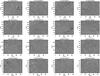 |
Fig. 1 Vertical magnetic field component Bz at 00:00 UT for all 16 SDO/HMI quiet-Sun magnetogram sequences in our study. White and black denote positive and negative magnetic field concentrations. Same dates correspond to quiet-Sun regions observed in different locations on the solar disk. |
2. Observations and methodology
2.1. Observations
For our analysis, we use 16 daily sequences of photospheric vector magnetograms of sizeable quiet-Sun regions, which were obtained with the Helioseismic and Magnetic Imager (HMI; Scherrer et al. 2012) onboard the Solar Dynamics Observatory (SDO; Pesnell et al. 2012). The HMI provides full disk (4096 × 4096) vector magnetograms with a spatial sampling of 0.5′′ per pixel. These are derived with a Milne-Eddington-based inversion approach (Borrero et al. 2011) from the observed four Stokes parameters (I, Q, U, and V) of the Fe i 617.3 nm photospheric line. To enhance the signal-to-noise ratio and suppress 5-min p-mode oscillations, 720-s filtergrams are used for the derivation of the Stokes parameters. The azimuthal 180° ambiguity of vector magnetograms was treated by means of the nonpotential field calculation (NPFC) of Georgoulis (2005), as revised by Metcalf et al. (2006). The heliographic components of the magnetic field vector on the heliographic plane, derived with the deprojection equations of Gary & Hagyard (1990) were used.
All 16 quiet-Sun regions are located close to the solar disk center to avoid major projection effects. They have been observed between December 2013 and July 2014, as systematic full disk SDO/HMI magnetograms were released from the SDO/HMI science team only after December 2013. The initial fixed field-of-view (hereafter FOV) of our sequences on the image plane covers a sizeable 586′′× 350′′ area (205 100 arcsec2) of the solar surface. Each used sequence comprises 120 images (daily sequences with a cadence of 720 s) with no corrections for solar rotation considered during the initial sequence selection. Hence, final deprojection and co-alignment of the sequence images resulted in effective area sizes on the heliographic plane ranging between 124 754 arcsec2 and 160 663 arcsec2 with a mean effective area of 143 138 arcsec2, almost half that of the initial FOV. The unsigned flux ranges between 7.2 × 10²¹ Mx and 2.5 × 10²² Mx with an average value of 1.5 × 10²² Mx, while the overall flux imbalance is 14 ± 7%. Scaled to the entire solar surface, it corresponds to an average total flux of 1.2 × 1024 Mx, which is on the higher end of the reported range for total unsigned flux in quiet Sun (see Gošić et al. 2014, and references therein).
Figure 1 shows a sample image at 00:00 UT for each SDO/HMI magnetogram daily sequence used in this analysis. As already mentioned in the Introduction, in quiet-Sun regions the magnetic field is mostly concentrated at the boundaries of supergranular cells that constitute the magnetic network. No such clearly visible cells are present in most of our images, however, most probably because during the selected period of study the Sun was, unfortunately, at the maximum phase of its cycle and areas were selected within latitudes of usually intense solar activity. Hence, most of the chosen near-equatorial quiet-Sun regions, are mainly the result of older, diffused ARs, justifying the somewhat higher than usual recorded quiet-Sun unsigned fluxes. As magnetic field magnitudes within the magnetic network are larger than field values within the interior of supergranular cells that define the IN, the total network area can be considered the area where the amplitude of the vertical field component Bz exceeds a threshold value. This threshold value is typically of the order of 100–300 G, with 200 G the most commonly used value in literature. In our analysis, given the lower resolution of SDO/HMI magnetograms compared to the SOT/SP magnetograms (Lites et al. 2008) from the Hinode satellite (a factor of four lower), we set this threshold value equal to 50 G, well above the SDO/HMI errors in magnetic field strength. The derived network area ranges between 1% and 18% of the total area with a mean value of 5%, a factor of two lower than the reported value of 10% for the network area during solar maximum (Caccin et al. 1998).
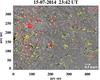 |
Fig. 2 Derived photospheric velocity field (yellow and red arrows) calculated with DAVE4VM for a vector magnetogram of the sequence of July 15, 2014, on top of a gray-scale image of the normal component of the magnetic field. A threshold of 0.07 km s-1 for velocities and 20 G for the magnetic field was used when plotting the velocity field. Black and white denotes positive and negative magnetic field concentrations, respectively. Yellow and red velocity arrows are associated with positive and negative fields, respectively. The white arrow at the bottom right corner indicates the velocity scale. |
2.2. Methodology for deriving magnetic energy and helicity rates
The helicity injection rate (Berger & Field 1984) depends both on the photospheric velocity field and the vector potential Ap of the potential magnetic field Bp with the same lower-boundary normal-field condition as the observed field B. The inference of the horizontal photospheric velocities, usually through local correlation tracking techniques (LCT; November & Simon 1988) applied in sequences of magnetograms, involves significant uncertainties (e.g., Welsch et al. 2007) mostly due to ambiguities in image motion.
Several other alternative methods for deriving photospheric plasma velocities have been proposed (see Welsch et al. 2007, and references therein) in an attempt to overcome two major deficiencies of LCT techniques: a) the underestimation of helicity injection by shear (Démoulin & Berger 2003); and b) their inconsistency with the magnetic induction equation governing the evolution of the photospheric magnetic fields (Schuck 2005). Both the Differential Affine Velocity Estimator method (DAVE) introduced by Schuck (2005, 2006) for LOS magnetograms and its generalization for vector magnetograms, the Differential Affine Velocity Estimator for Vector Magnetograms (DAVE4VM; Schuck 2008), estimate the plasma velocity υ using the normal component of the ideal induction equation. In the latter case, as the coordinate system for the derived affine velocity profile υ is not aligned with the magnetic field, only its perpendicular, cross-field component υ⊥, which plays a role in the induction equation, has to considered. Hence, the field-aligned plasma flow υ∥ = (υ·B)B/B2 has to be removed as υ⊥ = υ − υ∥. Figure 2 shows an example of the derived photospheric velocity field with DAVE4VM.
As Berger & Field (1984) have shown, the helicity flux  across the plane S of the magnetogram is derived by
 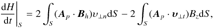 (1)where υ⊥ n and υ⊥ t are the normal and tangential components of υ⊥, B is the magnetic field vector with z denoting the normal (vertical) axis and h its horizontal x- and y-components on the tangential (horizontal) plane, and Ap is the corresponding current-free magnetic vector potential. The latter is calculated by means of a fast Fourier transform method, as implemented by Chae (2001). The first term of Eq. (1) roughly corresponds to the helicity flux through emergence and the second term to helicity flux through photospheric shuffling.
Likewise, as Kusano et al. (2002) have shown, the magnetic energy injection rate (i.e., the Poynting flux)  is given by
  (2)with the first term roughly corresponding to the energy flux through emergence and the second term to energy flux through shuffling.
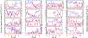 |
Fig. 3 Absolute helicity and the energy rate variation per network unit area (red and blue solid lines, and left and right ordinate, respectively) for our 16 daily SDO/HMI quiet-Sun magnetogram sequences (only the seventh magnetogram sequence starts later at 10:00 UT). For clarity in assessing the long-term evolution of helicity and energy rates, all shown curves are one-hour averages of the actual curves. The dotted red and blue lines denote the corresponding values of the mean helicity amplitude rate and energy rate per network unit area, respectively (see also Fig. 7). |
3. Results
3.1. Energy and helicity rates in quiet-Sun regions
Helicity is a signed quantity, so both left- and right-handed helicity can be injected and can be simultaneously present in a magnetic configuration. Hence, even in the extreme case of zero net (algebraic) helicity because of equal and opposite budgets of helicity injection, the absolute amplitude of helicity present, defined as the sum of both left- and right-handed helicity amplitudes, would be nonzero. Figure 3 shows the absolute helicity rate variation and the respective energy rate variation per network unit area for the 16 studied quiet-Sun magnetogram sequences. The total budgets of net helicity/energy and the total amounts of helicity amplitude accumulated within the day in each observed quiet region can be derived from the respective rates by multiplying with the network area and integrating in time. As the already existing budgets at the beginning of integration are unknown, exact estimates of the total helicity/energy budgets of each region are not possible.
In Fig. 3, all curves show significant scattering within the day around their median values, probably stemming from the stochastic nature of magnetic flux emergence in quiet-Sun regions, which is not as intense and localized as in ARs. As discussed in Gošić et al. (2014), there exists continuous emergence of small magnetic flux concentrations in the IN, combined with significant migration toward the network, with the IN supplying as much flux as present to the network and being able to replace the network’s entire flux within 18 to 24 h. In our case, the dynamical evolution is even quicker with important diffusion present in addition, as discussed below.
Figure 4 shows the ratio between the total accumulated net helicity within each studied region and the total accumulated amplitude of helicity. A ratio amplitude close to one implies the injection of a dominant sense of helicity. Tziotziou et al. (2014a) have shown, that contrary to ARs, there is no dominant sense of helicity present in quiet-Sun regions (helicity sense incoherence). The average ratio amplitude of our sample is 0.55, a rather high number as there exists a considerable number of quiet-Sun regions with a dominant (ratio amplitude ≥0.7) sense of helicity, probably stemming from the fact that these quiet-Sun regions are the remnants of diffused old ARs. Most of the helicity seems to be injected by shuffling motions rather than emergence, as Fig. 5 (black squares) that shows the ratio between the two amplitudes of the respective accumulated helicity terms, clearly suggests. The mean ratio between the amplitudes of helicity through shuffling and emergence is 2.3, which is much lower than the respective ratio in ARs with strong polarity inversion lines (PIL) where shear motions add large amounts of helicity through shuffling (Tziotziou et al. 2013). Both helicity incoherence and the dominance of helicity injection by shuffling over emergence are attributed to a) the nature and dynamics of magnetic flux emergence in quiet Sun, as discussed before, and b) a difference in the generating physical processes, with mostly near-surface and, hence, strongly dependant on near-surface flows generation of helicity in quiet-Sun compared to ARs. In ARs, helicity mostly emerges from the solar interior in dynamo-generated, highly-twisted magnetic flux tubes, when not also generated and/or complemented by strong shear motions in PILs.
The clear dominance of shuffling over emergence in helicity injection in quiet-Sun regions suggests that helicity rates derived with the computationally less expensive DAVE method (see Sect. 2.2) for LOS magnetograms, would not differ significantly from those derived by DAVE4VM for vector magnetograms. Application of both methods on the sequences of LOS and vector magnetograms of July 15, 2014 (Fig. 6) indeed shows a remarkable both qualitative and quantitative correspondence between respective results.
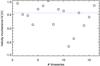 |
Fig. 4 Ratio between the total accumulated net helicity and the total accumulated amplitude of helicity for the 16 quiet-Sun regions, with negative and positive values denoting negative (left-handed) and positive (right-handed) accumulated net helicity, respectively. The blue dotted line denotes the mean absolute amplitude of this ratio. |
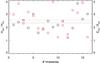 |
Fig. 5 Ratio between the accumulated amplitudes of helicity due to shuffling and emergence (black squares) and the corresponding ratio between the accumulated amplitudes of the respective energy terms (red squares) for the 16 quiet-Sun regions. The dotted black and red lines denote respective mean values. |
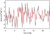 |
Fig. 6 Helicity rates calculated with DAVE4VM (black line) and DAVE (red line) from the vector and LOS magnetograms for the quiet-Sun sequence of July 15, 2014. |
Concerning the injection of energy, as Fig. 3 suggests, the majority of the studied quiet-Sun regions exhibit negative energy rates corresponding to energy removal, with only three (3) of them showing an overall positive energy injection. We can only conjecture that this could actually be associated with large ongoing diffusion processes as these quiet-Sun regions are remnants of old ARs and all studied quiet-Sun sequences exhibit a much quicker evolution than the reported 1.8 ± 0.9 day lifetime of supergranules. The ratio of amplitudes of energy injected by shuffling motions over energy injected by emergence (Fig. 5, red squares) shows, like helicity, a clear dominance of the shuffling term. This is in contrast to the respective behavior in ARs, in which the continuous emergence of large magnetic flux results in dominance of energy injected through emergence over shuffling (Tziotziou et al. 2013). The average ratio between the respective shuffling and emergence energy terms is 2.53 and could probably be attributed, like helicity, to the nature, dynamics, and magnitude of magnetic flux emergence in quiet-Sun regions (Schrijver et al. 1997; Gošić et al. 2014) combined with intense diffusion that mostly removes energy from the magnetic configuration.
3.2. Energy and helicity budgets of quiet-Sun regions
Figure 7 shows the helicity and energy rates per network unit area for each of the 16 quiet-Sun regions under study. These correspond to the mean values derived from the respective sequences of Fig. 3. Most of the derived helicity/energy rates per network unit area are quite consistent within errors, with only one clear outlier corresponding to the quiet-Sun region of March 6, 2014 (seventh region). This region exhibits much higher values, both in helicity and energy, and considerable errors. Furthermore, as Fig. 4 suggests, it exhibits a dominant sense of helicity (ratio equal to 1) like in ARs and contrary to the normal behavior of quiet Sun regions. As the corresponding magnetogram of Fig. 1 shows, this region is quite exceptional when compared to the others, with large patches of magnetic field concentrations, far from the familiar cell-like magnetic topology of supergranules in quiet-Sun regions.
Hence, for our analysis, hereafter, we consider the average values derived without the aforementioned outlier region. The average value of helicity rate per network unit area of all remaining 15 quiet-Sun regions is 2.70 ± 1.37 × 1015 Mx2 cm-2 s-1, while the average energy rate per network unit area for the two remaining regions with positive energy rates is 7.73 ± 3.67 × 10⁵ erg cm-2 s-1. The approximate mean values derived by Tziotziou et al. (2014a) are 1.25 × 1015 Mx2 cm-2 s-1 and 5.4 × 10⁵ erg cm-2 s-1. These are calculated from the corresponding coefficients B of their linear fit for a network threshold of 100 G (see their Fig. 4), that provide helicity/energy per network area, under the assumption that both helicity/energy replenish within the 1.8-day lifetime of supergranules. Both values are in good agreement with the values derived from the present analysis.
The derived free energy injection rate of 7.73 ± 3.67 × 10⁵ erg cm-2 s-1 and its subsequent use for the calculation of the quiet-Sun free magnetic energy budget over an entire solar cycle is of particular interest and used for comparison to previous results, as it is derived only from two quiet-Sun regions during solar maximum. Although it is in good agreement with the result of Tziotziou et al. (2014a), which was derived with a different method during solar minimum, further investigation is perhaps necessary during the next solar minimum when diffusive processes of ARs will be negligible.
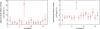 |
Fig. 7 Helicity amplitude (left panel) and energy (right panel) rates per network unit area and respective 1σ errors for all 16 SDO/HMI quiet-Sun regions under study. The dotted blue lines in both panels denote the average helicity energy rate value (3.85 ± 4.79 × 1015 Mx2 cm-2 s-1) of all 16 regions and the average energy rate value (2.23 ± 2.53 × 10⁶ erg cm-2 s-1) of all regions with positive energy rates. Errors are larger than the obtained average values due to the presence of the seventh region (see text). The dotted red lines denote the average helicity/energy rate value excluding this seventh, outlier, quiet-Sun region, which are finally used in our analysis. The light gray line in the right panel indicates the zero level. |
Assuming a sinusoidal variation of the network area between 10% and 25% within a solar cycle, as Fig. 3 of Caccin et al. (1998) suggests, we can derive the total quiet-Sun budgets for helicity and free magnetic energy in an entire solar cycle. The derived values of 9.1 ± 4.6 × 1045 Mx2 and 2.6 ± 1.2 × 1036 erg are of the same order as the respective values derived by Tziotziou et al. (2014a). These authors, however, used the calculated instantaneous budgets of helicity and energy and assumed that both quantities dissipate/replenish within the supergranular lifetime of 1.8 ± 0.9 days to calculate the corresponding rates. The derived solar-cycle helicity budget is almost three orders of magnitude higher than the value of ~1043 Mx2 reported by Welsch & Longcope (2003), who relied on a similar analysis using LOS magnetogram sequences and an order of magnitude higher than the approximate value of ~1.5 × 1044 Mx2 reported by Georgoulis et al. (2009). Georgoulis et al. (2009) used typical velocity and magnetic field values in the helicity rate equation. The aforementioned energy/helicity integration does not take the already existing budgets of free magnetic energy and relative magnetic helicity into account, hence, possibly even slightly larger amounts of energy/helicity could be available in quiet-Sun network regions.
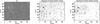 |
Fig. 8 Vertical magnetic field component Bz (left panel) for the vector magnetogram of July 15, 2014 at 23:42 UT, with white and black denoting positive and negative magnetic field concentrations. Respective derived gray-scale maps of the magnitude of energy injection density (middle panel) and the magnitude of helicity injection density (right panel) with black denoting high values. |
3.3. Are energy and helicity budgets in quiet Sun sufficient to power small-scale structure dynamics?
Figure 8 shows the two dimensional distributions of energy and helicity injection density magnitudes for the magnetogram of July 15, 2014 (23:42 UT), corresponding to the velocity field of Fig. 2. Both distributions suggest that generation of helicity and energy, governed by the photospheric velocity field, is mostly occurring along magnetic field concentrations that constitute the magnetic network. However, there is significant injection/generation of helicity/energy within the IN, which via flows continuously migrates toward the network boundaries where it finally merges and/or annihilates with the existing helicity/energy budgets (e.g., Gošić et al. 2014). The accumulated energy in the magnetic network could probably be dissipated in fine-scale structures residing at the supergranular boundaries, such as mottles and spicules (Tsiropoula et al. 2012), through dissipative processes, such as magnetic reconnection. This energy has been calculated to be at least 1.2 × 10⁵ erg cm-2 s-1 in mottles (Tsiropoula & Tziotziou 2004), while similar calculations for spicules by including cogenerated Alvén waves (Moore et al. 2011) also, resulted in a value of 7 × 10⁵ erg cm-2 s-1. Both these values are of the same order of magnitude as the value of 7.73 ± 3.67 × 10⁵ erg cm-2 s-1 derived in this analysis and the value of 5.4 × 10⁵ erg cm-2 s-1 (see Sect. 3.2 for details) derived by Tziotziou et al. (2014a), using the instantaneous budgets of energy and helicity. Hence, the derived free energy injection seems to be enough to power the dynamics of fine-scale structures and probably play a role in the heating of the chromosphere, which needs considerable amounts of energy (Tsiropoula & Tziotziou 2004).
There are no quantitative estimations of the helicity stored and/or carried by fine-scale structures, such as mottles and spicules, although there exist reports in literature (Jess et al. 2009; Curdt & Tian 2011; De Pontieu et al. 2012; Tsiropoula et al. 2012) that such structures often show a helical behavior. Recent observations with NASA’s Interface Region Imaging Spectrograph (IRIS) have shown that even the quiet-Sun chromosphere and transition region, in sub-arcsec scales, are filled with twist or torsional motions (De Pontieu et al. 2014). However, observations cannot confirm if and how these observed twists and torsional motions are related to possible manifestations of helicity presence and/or removal. Investigation of the association of reconnection-driven dynamics with the energy and helicity evolution has only been reported so far in larger-scale solar polar jet simulations in polar coronal holes (Pariat et al. 2009).
4. Discussion and conclusions
We have studied 16 daily sequences of quiet Sun vector magnetograms to derive the relative magnetic helicity and free magnetic energy injection, both from emergence and photospheric surface motion, in an attempt to a) simultaneously measure both quantities contrary to similar previous works by Welsch & Longcope (2003) and Georgoulis et al. (2009), which provided estimates only for the helicity; and b) to get a direct measure of these quantities without any assumptions concerning their temporal behavior, as in the work of Tziotziou et al. (2014a). As the selected regions fall within the maximum of the solar cycle, they all exhibit significant diffusion as possible remnants of older ARs, unsigned fluxes in the higher end of expected quiet Sun values and twice as low network coverage than previous studies reported. In conjunction with the continuous, but stochastic nature of magnetic flux emergence in quiet Sun, driven also by supergranular surface dynamics, all sequences show significant scattering around their median values and the majority of them show significant energy removal in the form of negative energy injection rates.
Our analysis suggests that a) quiet Sun regions exhibit no dominant sense of helicity injection; and b) helicity/energy generation in quiet Sun due to surface shuffling motions dominates over emergence. This is dictated, both by the nature and dynamics of magnetic flux emergence in the quiet Sun. There, continuous emergence in IN of small magnetic flux elements of the order of 1018 Mx, is followed by their continuous migration toward the network boundaries where they either merge or annihilate, depending on the polarity, with the existing network magnetic fields. Furthermore, it implies a difference in helicity generating mechanisms in quiet Sun and ARs, with near-surface generation as the most probable mechanism in quiet Sun, in contrast to deeper, dynamo-generation for ARs (emerging helical magnetic flux tubes) combined with further shear generation in PIL-dominated ARs.
The derived average values for helicity and energy rate per network unit area are in good agreement with the approximate values derived from Tziotziou et al. (2014a) using the instantaneous budgets of helicity/energy per network area and the assumption that these replenish within the supergranular lifetime. Consequently, the total quiet-Sun budgets in an entire solar cycle for magnetic helicity and free magnetic energy (9.1 ± 4.6 × 1045 Mx2 and 2.6 ± 1.2 × 1036 erg, respectively) are similar to the values derived by Tziotziou et al. (2014a). However, the derived helicity budget is almost three orders of magnitude higher than the value of ~1043 Mx2 derived by Welsch & Longcope (2003) and one order of magnitude higher than the approximate value of ~1.5 × 1044 Mx2 reported by Georgoulis et al. (2009). Although the derivation of Welsch & Longcope (2003) only corresponds to helicity generated through surface motions, as our analysis indicates, there is no significant difference (much less than an order of magnitude) between helicity through shuffling and total helicity (Figs. 5 and 6). Tziotziou et al. (2013) noticed that methods relying on photospheric flow velocities and respective helicity injection rates tend to underestimate the integrated helicity budgets in ARs compared to methods relying on instantaneous budgets. This, however, does not seem to be the case for quiet Sun regions, as both methods give similar results. It is hard to say if this is related to differences arising between the two used quiet-Sun samples (as the present one was selected during solar maximum, while the previous one during solar minimum) and the assumptions made, or indeed the method is more accurate for quiet Sun than ARs. As, however, similar calculations of Welsch & Longcope (2003) are almost three orders of magnitude lower, this suggests that sample selection probably does play an important role in the derived results.
The derived free magnetic energy rate per network unit area of 7.73 ± 3.67 × 10⁵ erg cm-2 s-1 is similar to the value of 5.4 × 10⁵ erg cm-2 s-1 (see Sect. 3.2 for details) derived by Tziotziou et al. (2014a) and of the same order as the energy needed to power mottles/spicules. The latter is equal to 1.2 × 10⁵ erg cm-2 s-1, according to Tsiropoula & Tziotziou (2004), and 7 × 10⁵ erg cm-2 s-1, according to Moore et al. (2011), when co-generated Alvén waves are included. With generation of both helicity and energy mostly concentrated along the network, our analysis suggests that there is sufficient free energy in the network to power fine-scale structures residing at the network via dissipative processes, such as magnetic reconnection. Although there is currently substantial observational evidence (Jess et al. 2009; Curdt & Tian 2011; De Pontieu et al. 2012; Tsiropoula et al. 2012; De Pontieu et al. 2014) for the presence of helical behavior and twist in small structures, such as mottles and spicules, complemented by some simulations on larger polar-jet structures (Pariat et al. 2009), there are no quantitative estimates of this helicity. However, our present analysis suggests an available helicity of 2.70 ± 1.37 × 1015 Mx2 cm-2 s-1 in network areas, which is close to the value of 1.25 × 1015 Mx2 cm-2 s-1 reported by Tziotziou et al. (2014a). Verification of these values is still pending and as the three-dimensional magnetic field configuration cannot be inferred from observations, it relies on a combination of high-resolution magneto-hydrodynamic helicity simulations in fine-scale structures with high-resolution chromospheric observations.
Acknowledgments
The data are used courtesy of NASA/SDO and the HMI science team. The research was funded through the project “SOLAR-4068”, which is implemented under the “ARISTEIA II” Action of the operational program “Education and Lifelong Learning” and is co-funded by the European Social Fund (ESF) and Greek national funds.
References
- Berger, M. A. 1984, Ph.D. Thesis Harvard Univ., Cambridge, MA [Google Scholar]
- Berger, M. A. 1999, Plasma Physics and Controlled Fusion, 41, 167 [Google Scholar]
- Berger, M. A., & Field, G. B. 1984, J. Fluid Mech., 147, 133 [NASA ADS] [CrossRef] [Google Scholar]
- Borrero, J. M., Tomczyk, S., Kubo, M., et al. 2011, Sol. Phys., 273, 267 [Google Scholar]
- Caccin, B., Ermolli, I., Fofi, M., & Sambuco, A. M. 1998, Sol. Phys., 177, 295 [NASA ADS] [CrossRef] [Google Scholar]
- Chae, J. 2001, ApJ, 560, L95 [NASA ADS] [CrossRef] [Google Scholar]
- Curdt, W., & Tian, H. 2011, A&A, 532, L9 [NASA ADS] [CrossRef] [EDP Sciences] [Google Scholar]
- Démoulin, P., & Berger, M. A. 2003, Sol. Phys., 215, 203 [NASA ADS] [CrossRef] [Google Scholar]
- De Pontieu, B., Carlsson, M., Rouppe van der Voort, L. H. M., et al. 2012, ApJ, 752, L12 [NASA ADS] [CrossRef] [Google Scholar]
- De Pontieu, B., Rouppe van der Voort, L., McIntosh, S. W., et al. 2014, Science, 346, 1255732 [CrossRef] [Google Scholar]
- DeVore, C. R. 2000, ApJ, 539, 944 [NASA ADS] [CrossRef] [Google Scholar]
- Finn, J. M., & Antonsen, T. M., Jr. 1985, Commun. Plasma Phys. Controlled Fusion, 9, 111 [Google Scholar]
- Galsgaard, K., Parnell, C. E., & Blaizot, J. 2000, A&A, 362, 395 [NASA ADS] [Google Scholar]
- Gary, G. A., & Hagyard, M. J. 1990, Sol. Phys., 126, 21 [NASA ADS] [CrossRef] [Google Scholar]
- Georgoulis, M. K. 2005, ApJ, 629, L69 [NASA ADS] [CrossRef] [Google Scholar]
- Georgoulis, M. K., Rust, D. M., Pevtsov, A. A., Bernasconi, P. N., & Kuzanyan, K. M. 2009, ApJ, 705, L48 [NASA ADS] [CrossRef] [Google Scholar]
- Georgoulis, M. K., Tziotziou, K., & Raouafi, N.-E. 2012, ApJ, 759, 1 [NASA ADS] [CrossRef] [Google Scholar]
- Gošić, M., Bellot Rubio, L. R., Orozco Suárez, D., Katsukawa, Y., & del Toro Iniesta, J. C. 2014, ApJ, 797, 49 [NASA ADS] [CrossRef] [Google Scholar]
- Jess, D. B., Mathioudakis, M., Erdélyi, R., et al. 2009, Science, 323, 1582 [NASA ADS] [CrossRef] [PubMed] [Google Scholar]
- Kusano, K., Maeshiro, T., Yokoyama, T., & Sakurai, T. 2002, ApJ, 577, 501 [NASA ADS] [CrossRef] [Google Scholar]
- Lites, B. W., Kubo, M., Socas-Navarro, H., et al. 2008, ApJ, 672, 1237 [NASA ADS] [CrossRef] [Google Scholar]
- Low, B. C. 1994, Phys. Plasmas, 1, 1684 [NASA ADS] [CrossRef] [Google Scholar]
- Metcalf, T. R., Leka, K. D., Barnes, G., et al. 2006, Sol. Phys., 237, 267 [Google Scholar]
- Metcalf, T. R., De Rosa, M. L., Schrijver, C. J., et al. 2008, Sol. Phys., 247, 269 [Google Scholar]
- Meyer, K. A., Sabol, J., Mackay, D. H., & van Ballegooijen, A. A. 2013, ApJ, 770, L18 [NASA ADS] [CrossRef] [Google Scholar]
- Moore, R. L., Sterling, A. C., Cirtain, J. W., & Falconer, D. A. 2011, ApJ, 731, L18 [NASA ADS] [CrossRef] [Google Scholar]
- November, L. J., & Simon, G. W. 1988, ApJ, 333, 427 [Google Scholar]
- Pariat, E., Antiochos, S. K., & DeVore, C. R. 2009, ApJ, 691, 61 [NASA ADS] [CrossRef] [Google Scholar]
- Parnell, C. E. 2001, Sol. Phys., 200, 23 [NASA ADS] [CrossRef] [Google Scholar]
- Pesnell, W. D., Thompson, B. J., & Chamberlin, P. C. 2012, Sol. Phys., 275, 3 [NASA ADS] [CrossRef] [Google Scholar]
- Rieutord, M., & Rincon, F. 2010, Liv. Rev. Sol. Phys., 7, 2 [Google Scholar]
- Scherrer, P. H., Schou, J., Bush, R. I., et al. 2012, Sol. Phys., 275, 207 [Google Scholar]
- Schrijver, C. J., & Harvey, K. L. 1994, Sol. Phys., 150, 1 [NASA ADS] [CrossRef] [Google Scholar]
- Schrijver, C. J., Title, A. M., van Ballegooijen, A. A., Hagenaar, H. J., & Shine, R. A. 1997, ApJ, 487, 424 [NASA ADS] [CrossRef] [Google Scholar]
- Schrijver, C. J., De Rosa, M. L., Metcalf, T. R., et al. 2006, Sol. Phys., 235, 161 [Google Scholar]
- Schuck, P. W. 2005, ApJ, 632, L53 [NASA ADS] [CrossRef] [Google Scholar]
- Schuck, P. W. 2006, ApJ, 646, 1358 [NASA ADS] [CrossRef] [Google Scholar]
- Schuck, P.W. 2008, ApJ, 683, 1134 [NASA ADS] [CrossRef] [Google Scholar]
- Tsiropoula, G., & Tziotziou, K. 2004, A&A, 424, 279 [NASA ADS] [CrossRef] [EDP Sciences] [Google Scholar]
- Tsiropoula, G., Tziotziou, K., Kontogiannis, I., et al. 2012, Space Sci. Rev., 169, 181 [NASA ADS] [CrossRef] [Google Scholar]
- Tziotziou, K., Georgoulis, M. K., & Raouafi, N.-E. 2012, ApJ, 759, L4 [NASA ADS] [CrossRef] [Google Scholar]
- Tziotziou, K., Georgoulis, M. K., & Liu, Y. 2013, ApJ, 772, 115 [NASA ADS] [CrossRef] [Google Scholar]
- Tziotziou, K., Tsiropoula, G., Georgoulis, M. K., & Kontogiannis, I. 2014a, A&A, 564, A86 [NASA ADS] [CrossRef] [EDP Sciences] [Google Scholar]
- Tziotziou, K., Moraitis, K., Georgoulis, M. K., & Archontis, V. 2014b, A&A, 570, L1 [NASA ADS] [CrossRef] [EDP Sciences] [Google Scholar]
- Wang, H., Tang, F., Zirin, H., & Wang, J. 1996, Sol. Phys., 165, 223 [NASA ADS] [CrossRef] [Google Scholar]
- Welsch, B. T., & Longcope, D. W. 2003, ApJ, 588, 620 [NASA ADS] [CrossRef] [Google Scholar]
- Welsch, B. T., Abbett, W. P., De Rosa, M. L., et al. 2007, ApJ, 670, 1434 [NASA ADS] [CrossRef] [Google Scholar]
- Woodard, M. F., & Chae, J. 1999, Sol. Phys., 184, 239 [NASA ADS] [CrossRef] [Google Scholar]
- Zhao, M., Wang, J.-X., Jin, C.-L., & Zhou, G.-P. 2009, RA&A, 9, 933 [Google Scholar]
All Figures
|
Fig. 1 Vertical magnetic field component Bz at 00:00 UT for all 16 SDO/HMI quiet-Sun magnetogram sequences in our study. White and black denote positive and negative magnetic field concentrations. Same dates correspond to quiet-Sun regions observed in different locations on the solar disk. |
| In the text | |
|
Fig. 2 Derived photospheric velocity field (yellow and red arrows) calculated with DAVE4VM for a vector magnetogram of the sequence of July 15, 2014, on top of a gray-scale image of the normal component of the magnetic field. A threshold of 0.07 km s-1 for velocities and 20 G for the magnetic field was used when plotting the velocity field. Black and white denotes positive and negative magnetic field concentrations, respectively. Yellow and red velocity arrows are associated with positive and negative fields, respectively. The white arrow at the bottom right corner indicates the velocity scale. |
| In the text | |
|
Fig. 3 Absolute helicity and the energy rate variation per network unit area (red and blue solid lines, and left and right ordinate, respectively) for our 16 daily SDO/HMI quiet-Sun magnetogram sequences (only the seventh magnetogram sequence starts later at 10:00 UT). For clarity in assessing the long-term evolution of helicity and energy rates, all shown curves are one-hour averages of the actual curves. The dotted red and blue lines denote the corresponding values of the mean helicity amplitude rate and energy rate per network unit area, respectively (see also Fig. 7). |
| In the text | |
|
Fig. 4 Ratio between the total accumulated net helicity and the total accumulated amplitude of helicity for the 16 quiet-Sun regions, with negative and positive values denoting negative (left-handed) and positive (right-handed) accumulated net helicity, respectively. The blue dotted line denotes the mean absolute amplitude of this ratio. |
| In the text | |
|
Fig. 5 Ratio between the accumulated amplitudes of helicity due to shuffling and emergence (black squares) and the corresponding ratio between the accumulated amplitudes of the respective energy terms (red squares) for the 16 quiet-Sun regions. The dotted black and red lines denote respective mean values. |
| In the text | |
|
Fig. 6 Helicity rates calculated with DAVE4VM (black line) and DAVE (red line) from the vector and LOS magnetograms for the quiet-Sun sequence of July 15, 2014. |
| In the text | |
|
Fig. 7 Helicity amplitude (left panel) and energy (right panel) rates per network unit area and respective 1σ errors for all 16 SDO/HMI quiet-Sun regions under study. The dotted blue lines in both panels denote the average helicity energy rate value (3.85 ± 4.79 × 1015 Mx2 cm-2 s-1) of all 16 regions and the average energy rate value (2.23 ± 2.53 × 10⁶ erg cm-2 s-1) of all regions with positive energy rates. Errors are larger than the obtained average values due to the presence of the seventh region (see text). The dotted red lines denote the average helicity/energy rate value excluding this seventh, outlier, quiet-Sun region, which are finally used in our analysis. The light gray line in the right panel indicates the zero level. |
| In the text | |
|
Fig. 8 Vertical magnetic field component Bz (left panel) for the vector magnetogram of July 15, 2014 at 23:42 UT, with white and black denoting positive and negative magnetic field concentrations. Respective derived gray-scale maps of the magnitude of energy injection density (middle panel) and the magnitude of helicity injection density (right panel) with black denoting high values. |
| In the text | |
Current usage metrics show cumulative count of Article Views (full-text article views including HTML views, PDF and ePub downloads, according to the available data) and Abstracts Views on Vision4Press platform.
Data correspond to usage on the plateform after 2015. The current usage metrics is available 48-96 hours after online publication and is updated daily on week days.
Initial download of the metrics may take a while.