| Issue |
A&A
Volume 581, September 2015
|
|
|---|---|---|
| Article Number | A109 | |
| Number of page(s) | 12 | |
| Section | Cosmology (including clusters of galaxies) | |
| DOI | https://doi.org/10.1051/0004-6361/201526289 | |
| Published online | 16 September 2015 | |
Time variations of narrow absorption lines in high resolution quasar spectra ⋆
1
Sorbonne Universités, UPMC Univ. Paris 06, UMR 7095, Institut
d’Astrophysique de Paris,
75014
Paris,
France
e-mail:
This email address is being protected from spambots. You need JavaScript enabled to view it.
2
CNRS, UMR 7095, Institut d’Astrophysique de Paris,
75014
Paris,
France
3
UCO/Lick Observatory, UC Santa Cruz, Santa Cruz, CA
95064,
USA
4
Aix-Marseille Université, CNRS, LAM (Laboratoire d’Astrophysique
de Marseille) UMR 7326, 13388
Marseille,
France
5
Department of Astronomy, University of Chicago,
5640 South Ellis Avenue,
Chicago, IL
60637,
USA
Received: 9 April 2015
Accepted: 28 May 2015
Abstract
Aims. We have searched for temporal variations of narrow absorption lines in high resolution quasar spectra. A sample of five distant sources were assembled, for which two spectra are available, either VLT/UVES or Keck/HIRES, which were taken several years apart.
Methods. We first investigate under which conditions variations in absorption line profiles can be detected reliably from high resolution spectra and discuss the implications of changes in terms of small-scale structure within the intervening gas or intrinsic origin. The targets selected allow us to investigate the time behaviour of a broad variety of absorption line systems by sampling diverse environments: the vicinity of active nuclei, galaxy halos, molecular-rich galaxy disks associated with damped Lyα systems, as well as neutral gas within our own Galaxy.
Results. Intervening absorption lines from Mg ii, Fe ii, or proxy species with lines of lower opacity tracing the same kind of (moderately ionised) gas appear in general to be remarkably stable (1σ upper limits as low as 10% for some components on scales in the range 10–100 au), even for systems at zabs ≈ ze. Marginal variations are observed for Mg ii lines towards PKS 1229−021 at zabs = 0.83032; however, we detect no systems that display any change as large as those reported in low resolution SDSS spectra. The lack of clear variations for low β Mg ii systems does not support the existence of a specific population of absorbers made of swept-up gas towards blazars. In neutral or diffuse molecular media, clear changes are seen for Galactic Na i lines towards PKS 1229−02 (decrease in N by a factor of four for one of the five components over 9.7 yr), corresponding to structure on a scale of about 35 au, in good agreement with known properties of the Galactic interstellar medium. Tentative variations are detected for H2J = 3 lines towards FBQS J2340−0053 at zabs = 2.05454 (≃35% change in column density, N, over 0.7 yr in the rest frame), suggesting there is structure at the 10 au-scale for this warm molecular gas. A marginal change is also seen in C i from another velocity component of the same absorption system (≃70% variation in N(C i).
Key words: quasars: absorption lines / ISM: structure
Based on observations with UVES on the Very Large Telescope at the European Southern Observatory (under programs 67.C-0157, 68.A-0170, 074.B-0358, 278.A-5048, 082.A-0569, 087.A-0597, and 087.A-0778) and with HIRES on the Keck Telescope.
© ESO, 2015
1. Introduction
Absorption lines in distant active galactic nuclei (AGN) spectra have long been recognised as an invaluable source of information on diffuse material lying along these lines of sight (LoS), from local interstellar material within the Milky Way, disks or halos of intervening galaxies, intergalactic clouds, up to gas located in the vicinity of the AGN itself. As illustrated by numerous studies (see e.g. Noterdaeme et al. 2007; Neeleman et al. 2015), many properties of the gas can be investigated through a detailed analysis of the absorption lines, including ionisation level, chemical composition, density, and temperature.
Aside from the broad absorption lines (BAL) and intrinsic narrow absorption lines that often display time variations on timescales of months or years in the absorber’s frame (Hamann et al. 2008, 2011; Filiz Ak et al. 2013 and references therein; Misawa et al. 2014; Grier et al. 2015), intervening absorption systems observed in quasar spectra are thought to be essentially stable in time. However, a recent study based on multi-epoch low resolution SDSS spectra (Hacker et al. 2013) suggests that some narrow intervening systems (mainly Mg ii and Fe ii) might also display variability. These authors propose that time changes are due to the transverse motion of the LoS through the absorber coupled to the presence of structure in the absorbing gas at scales in the range 10–100 au, similar to what is observed for diffuse neutral gas in our own Galaxy (Crawford 2003; Lauroesch 2007; Welty 2007; Meyer et al. 2012). Indeed, transverse peculiar velocity values of a few 100 km s-1 are expected for the target, the observer, and the intervening gas, which imply drifts over a few years falling in this range. (We recall that 1 au yr-1 is equivalent to 4.67 km s-1.)
Information on spatial structure within the low-ionisation medium similar to the one probed by multi-epoch SDSS spectra remains quite limited. Observations of gravitationally lensed quasars with multiple images have been used to investigate spatial variations on scales of a few 100 pc. In particular, Rauch et al. (2002) studied the behaviour of Mg ii–Fe ii systems along three adjacent LoS towards Q2237+0305 and, by comparing the line profiles, infer a lower limit of about 0.5 kpc for the overall absorber extent and a typical size of the order of 100 pc for cloudlets associated with individual velocity components. Similarly, towards the lensed quasi-stellar object (QSO) pair APM 08279+5255, Kobayashi et al. (2002) derived an estimate for the cloudlet size of 200 pc, in good agreement with values inferred from earlier modelling of these absorbers (Churchill & Charlton 1999; Crighton et al. 2015). Such observations are restricted to a few systems and do not enable a study of the structure on smaller scales. In our own Galaxy, structure in the low-ionisation medium has been investigated by Welty (2007), who found no change in O i, Si ii, S ii, and Fe ii lines over tens of au. Thus, the limited information available (see also the recent study by Neeleman et al. 2015) does not suggest the presence of significant structure on scales as small as 100 au in the low-ionisation medium, comparable to the one seen in the neutral medium.
The results obtained by Hacker et al. (2013) then appear somewhat puzzling and require additional investigations. Their study is based on low resolution SDSS spectra, which can only provide equivalent width measurements and do not give access to the true line profiles and to the identification of the individual absorption velocity components. If some absorption lines do vary, changes most probably affect only some velocity components and should be much more apparent in high resolution spectra. High resolution line profiles would also be very useful for assessing the reality of any variation detection. Indeed, when spectral profiles are resolved (or at least partially resolved), changes in a specific transition from a given species imply a corresponding change for other transitions from the same species that can be computed a priori, providing a stringent reliability test. Furthermore, high resolution data will minimise the impact of various artefacts like imperfect sky subtraction, bad pixels, etc.
Good signal-to-noise (S/N) high resolution quasar spectra have been taken routinely over the past 15 yr (for instance, in the context of Large Programs conducted on 8–10 m class telescopes; see e.g. Bergeron et al. 2004; Molaro et al. 2013) and for some distant sources, several observations have been performed over time intervals reaching ten years. We have thus gathered a sample of five sources with at least two VLT/UVES or Keck/HIRES spectra taken several years apart. In one case, we acquired a spectrum specifically for this study. These LoS all together include a broad variety of systems, probing various environments ranging from neutral Galactic gas, galaxy disks at intermediate redshifts (i.e. damped Lyα system), Mg ii-Fe ii systems due to intervening galaxy halos, as well as systems with a redshift close to the emission redshift. Several of our targets fall in the blazar category, which will allow us to investigate the possible presence of narrow systems with a high ejection velocity, in line with the scenario put forward by Bergeron et al. (2011).
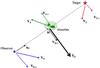 |
Fig. 1 Observer and target move with 3D velocities VO and VT in the cosmological frame. Their transverse component VO ⊥ and VT ⊥ determines the transverse velocity VM ⊥ of the impact point M. The latter combines with the transverse velocity of the absorber VA ⊥ to define the relative drift velocity of the LoS with respect to the gas, Vd, which sets the scale probed within the absorber during a given time interval. |
The purpose of our study is to explore the potential of multi-epoch high-resolution observations of AGN to investigate the small-scale structure in intervening gas and possible intrinsic variations for narrow low ejection velocity systems. In Sect. 2, we describe the method (expected LoS drifts, selection of transitions that are best suited for a search of variations, etc.) while the data and raw results are presented in Sect. 3. Their implications are discussed in Sect. 4. We summarise our results and mention some prospects for further variability studies in Sect. 5.
2. Detecting absorption line variations
When considering two spectra of the same target taken over some time interval, an important parameter is the drift of the LoS relative to a foreground absorber. We first discuss how one can estimate this scalelength, over which the comparison of the two observations will provide structure information. Next, we examine which line parameters (the opacity in particular) yield the best sensitivity to a given fractional column density change. Finally, we discuss methods that can be used to reliably detect line variations and assess their significance.
2.1. Line of sight drifts relative to the absorber
For now, we consider that the target is point-like and that it defines an “ideal” LoS, intersecting an intermediate-redshift absorber at point M (hereafter the “impact point”; Fig. 1). As mentioned above, it is the combination of small-scale density or velocity structure in the intervening gas and the transverse motion of the LoS through this material that can potentially induce line variations. The appropriate frame for computing the velocities of interest is a cosmological one, in which the cosmic microwave background (CMB) is globally isotropic. The motion of both the target and the observer determines the drift of the LoS in this frame. The observer’s motion is due mainly to the peculiar motion of the Milky Way and to Galactic rotation. The combination of the two corresponding velocities is directly constrained by the detection of the dipolar anisotropy in the CMB radiation, indicating that the solar system is moving at 368 ± 2 km s-1 relative to the observable Universe towards the direction lo = 263.85deg and bo = 48.25deg (Fixsen et al. 1996).
We denote by VO the corresponding velocity vector. Consider a target T with Galactic coordinates (lT,bT) and let uT be the unit vector pointing in this direction (Fig. 1). We are only concerned by the transverse component, thus by the projection, VO ⊥, of VO onto a plane normal to uT.
The sample.
This projected velocity can be written as  (1)where VO = VO.uO. From these relations, and using the components (cosbTcoslT, cosbTsinlT, sinbT) of the unit vector associated with Galactic coordinates (lT,bT), it is straightforward to compute VO, ⊥ for any specific target (for the five targets listed in Table 1, VO, ⊥ = 288,368,129,365, and 12 km s-1, respectively). In the most favourable case for which VO, ⊥ = VO, this motion alone results in a shift of about 4 × 10⁻³ pc or 800 au near the observer, over a time interval of ten years.
Unfortunately, we cannot estimate the transverse velocity of the target because the proper motion onto the sky is much too small to be measurable, contrary to interstellar medium studies, in which the proper motion of nearby bright stars is known. Unless the target belongs to a peculiar environment like a galaxy cluster or has experienced an ejection event, the magnitude of its peculiar velocity should be also a few 100 km s-1. The transverse velocity of the impact point M can then be written as  (2)where α = dA/dT, dA as the distance to the absorber and dT the distance to the target. Finally, one must take the velocity VA of the absorber into account in the cosmological frame or rather its transverse component, VA ⊥. In the end, the value of interest is the relative drift velocity
  (3)Again, VA ⊥ cannot be determined (interstellar studies suffer from the same difficulty), and only a typical value of a few hundred km s-1 can be considered. As with the observer, the actual value results from the combination of the bulk intervening galaxy motion and of the absorbing gas internal kinematics, e.g. rotation, infall, or outflow. A maximum value for the drift velocity Vd can be estimated assuming an optimal configuration in which VO ⊥ and VT ⊥ are parallel, while VA ⊥ points in the opposite direction. In that case, Vd can reach values Vd = max (VO ⊥,VT ⊥) + VA ⊥, as large as about 500 km s-1.
Equations (2) and (3) are valid in the local 3D space. On large cosmological scales, there is no unique way to define distances. Thus, these relations can hold only at low redshifts where all cosmological distances become equivalent. Since the exact values of both VT ⊥ and VA ⊥ are unknown for any specific target, it is sufficient for our purpose to estimate drift velocities by i) inserting typical values for VT ⊥ and VA ⊥ into the above equations; ii) using the angular size distance for d; and iii) taking time dilation into account: a time interval Δt in the observer’s frame corresponds to Δt/ (1 + zA) or Δt/ (1 + zT) in the absorber’s or target’s frame respectively, which is equivalent to reduce VA ⊥ and VT ⊥ by a factor of (1 + zA) or (1 + zT).
In fact, a quasar is an extended continuum source with a typical size in the range 10–100 au (the size of the accretion disk responsible for the optical emission; Dai et al. 2010). Thus, unlike observations of moving stars used to probe interstellar gas structure, significant averaging of the foreground structure can occur, implying a reduced amplitude for absorption line variations. The situation may be different for blazars. These sources undergo spectacular photometric variations and, when in a “high state”, their continuum is dominated by emission from the relativistic jet. Changes in the morphology of the source itself can also occur, which would be equivalent to an additional contribution to the drift of the LoS. Time changes in the 21 cm absorption seen towards AO 0235+164 and PKS 1127−14 by Wolfe et al. (1982) and Kanekar & Chengalur (2001) are attributed precisely to such an effect.
When dealing with absorption by Galactic interstellar material (four out of our five selected targets display relatively strong Ca ii or Na i absorption from Milky Way gas), the appropriate frame to consider is the local standard of rest (LSR), in which interstellar gas is at rest on average. In this case, the drift of the LoS is determined by the peculiar motion of the Sun in this frame, VS, or more specifically, by its projection onto a plane perpendicular to the LoS considered. This question is discussed in more detail in Boissé et al. (2013).
2.2. Sensitivity to absorption line variations
To select the absorption lines that are best suited to searching for time variations, we now quantify the sensitivity to a given fractional column density (N) change. Obviously, very weak or, in contrast, saturated features will be of little use: there must be some optimal intermediate value for the opacity.
Consider a fully resolved normalised profile, In(v), expressed in the velocity scale, 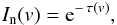 (4)where τ(v) is the line opacity at velocity v, written as
  (5)where k is a constant, λ0 the rest wavelength of the transition, f the oscillator strength, and N(v) dv the column density for species within the velocity interval [ v,v + dv ]. Let us first assume a spectrum noise that is independent of In. The sensitivity can then be expressed as
 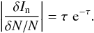 (6)It reaches its maximum at τ = 1, for which In ≈ 0.37. The interval over which the sensitivity is reduced by less than 20% is 0.61 ≤ τ ≤ 1.53, which corresponds to 0.22 ≤ In ≤ 0.54.
An alternative case of interest is that of photon noise, for which the spectrum rms follows a  law. The ability to detect a given variation δIn is then proportional to
 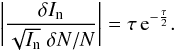 (7)This expression reaches its maximum at τ = 2, where In ≈ 0.14 (the sensitivity remains good in the sense defined above for 1.2 ≤ τ ≤ 3.1). In practice, observed spectra are within these two extreme cases, so we conclude that the sensitivity for the detection of variations is optimal for intermediate opacity values (typically 1.5), corresponding to normalised intensities of about 0.2.
One should keep in mind that, depending on the instrumental resolution and Doppler b parameter value, absorption profiles will generally not be fully resolved, implying apparent opacities that are lower than the true ones (Savage & Sembach 1991). For instance, with an instrumental resolution of 6.6 km s-1, the depth of a Gaussian line is reduced by a factor of 0.45 for b = 2 km s-1. Then, if the true opacity at line centre is τ0 = 1, the apparent opacity becomes 0.33. Therefore, to conclude on the sensitivity of a given line to changes in N, one cannot rely only on its observed profile. Fortunately, several transitions from the same species are often available with various f values. Simultaneous fitting of the corresponding line profiles will then allow us to determine the true opacity and assess whether these transitions are appropriate for a variability search.
2.3. Characterisation of line variations
Our aim is to detect line profile variations and to quantify their significance. A first direct indication can be obtained by superposing the two successive spectra after careful normalisation and adjustment of the wavelength scales if necessary. Such a raw comparison is meaningful only if the spectral resolution, R, is the same at the two epochs. If this is not the case, the higher R spectrum has to be degraded to the lower resolution value. Fortunately, the HIRES and UVES data used in this paper have very similar nominal resolutions – FWHM = 6.25 and 6.6 km s-1, respectively, and we could verify that, given the S/N, such a slight difference has a negligible effect on the profile of the absorption features discussed in this paper (cf. Sect. 3). Differences in the line spread function (LSF) might also play a role. One can use unresolved lines to check that such an effect does not affect the comparison of successive profiles.
It turns out that for the systems investigated here, the two successive spectra available rarely display marked, unambiguously significant differences. Thus, in order to i) increase our ability to detect weak variations by relying on the presence of several transitions from a given species (e.g. Fe ii, or H2); and ii) take differing R values into account if necessary, a more powerful method is to simultaneously fit all profiles corresponding to these transitions at each epoch. To this purpose, we used VPFIT1 a routine that uses multi-component Voigt profiles (convolved with the instrument profile, which we assume to be Gaussian here) and that yields the redshift zi, column density Ni, and Doppler parameter bi for each velocity component, together with their 1σ uncertainties. Comparison of the values obtained for each epoch then allows us to determine whether some of these parameters have undergone significant time changes. In all cases, the same sets of components were appropriate for fitting the profiles at both epochs with no significant change in zi or in bi.
Some time variations in Ni are detected or suspected for a few absorptions systems (see Sect. 3). To assess their significance, we computed the difference between epoch 1 and 2, ΔNi = Ni,2−Ni,1 and its uncertainty σ(ΔNi) by combining uncertainties on Ni,1 and Ni,2 in quadrature. This procedure provides a formal significance that properly takes the noise level in both spectra into account. Other sources of uncertainty related to continuum placement or to the choice of velocity components are more difficult to quantify, especially when variations are small. As a conservative approach, variations with a significance level above 3.5σ and an associated relative column density variation, ΔN/⟨N ⟩, above 25% are qualified as “significant”. Variations at more than 2σ but that do not fulfil these two criteria are considered as “marginal”.
When several transitions from the same species are available, the quality of the fit obtained provides a stringent test of the internal consistency of the data and gives a powerful way to rule out false variations due to instrumental artefacts. Indeed, changes must not only be present for all transitions but their magnitude must also be consistent with the f values. In this regard, species such as Fe ii, C i, or H2, which display many transitions from a given level within a relatively narrow wavelength interval, are especially suitable for probing weakly ionised, neutral, or molecular gas, respectively.
Often, several species can be used to trace a given phase (e.g. Mg ii, Fe ii, S ii for weakly ionised gas). One can then select among all lines detected from these species those i) whose opacity falls in the optimal range discussed above; and ii) that occur in spectral regions of good S/N.
Absorption systems.
Targets with absorption systems showing marginal or significant variability.
3. Variability study of five blazars with low-moderate β systems
3.1. The absorber sample
One of our initial motivations was to explore the link between gas swept by the AGN jet and low β absorbers, as suggested by Bergeron et al. (2011). We then investigated among their blazar sample objects with jets, thus radio-loud and γ-ray emitters (detected by Egret, Integral or Fermi/LAT). An additional selection criterion is the existence of Mg ii absorption systems at low relative velocity β ≡ Δv(zem,zabs) /c< 0.15 with a rest-frame equivalent width Wr(2796) > 0.3 Å, as well as intervening systems and Damped Ly-α (DLA) systems at high β. We then searched the VLT-UVES and Keck-HIRES archives for high-spectral resolution spectra of this blazar subsample, and selected targets observed several years apart, possibly about one decade. We checked that the S/N per pixel was S/N ≳ 10 for the main absorptions of interest: the Mg ii doublets at β< 0.15 and the Galactic Na i doublets.
One blazar satisfying the above selection criteria, is the extensively studied, highly variable BL Lac object AO 0235+164 for which variations of 21 cm intervening absorption at zabs = 0.524 had been reported three decades ago (Wolfe et al. 1982). This absorber has been identified as a BAL quasar with very faint extended emission (Burbidge et al. 1996). The variations were interpreted as most probably due to variations in the brightness distribution of the background radio source. Another blazar is PKS 1741−038, which was re-observed by us with UVES in 2011 to search for variability of its two strong Mg ii absorbers at β = 0.074 and 0.287. For both objects, the available UVES and HIRES spectra have been obtained at epochs about 9.5 yr apart in the observer’s frame.
We also searched for high resolution spectra of PKS 1229−02, a blazar for which we obtained deep HST imaging showing optical emission associated with knots in the radio jet (Le Brun et al. 1997). There is a DLA system at zabs = 0.3950 with associated 21 cm absorption, and several Mg ii absorbers at β ≤ 0.15. The above selection criteria are also met for this source and there are two sets of high S/N UVES spectra taken at epochs 9.2 yr apart.
Finally, there are HIRES and UVES data available for two targets with C i absorption at zabs ~ 1.5 with associated 21 cm absorption at high β (Kanekar et al. 2010): PKS 0458−020 (zabs = 1.5606) and FBQS J2340−0053 (zabs = 1.3608), the latter with observations about two years apart. In the radio spectrum of PKS 0458−020, variable 21 cm absorption on time-scale of months has been detected at zabs = 2.0395 (Kanekar et al. 2014, and references therein). There are also DLA systems at low β ≤ 0.10 toward PKS 0458−020 at zabs = 2.0395 and FBQS J2340−0053 at zabs = 2.0545. The physical conditions in the low β DLA system of FBQS J2340−0053, with associated C i absorption, have been investigated by Jorgenson et al. (2010). The multiple system at zabs = 1.3608 toward FBQS J2340−0053 has been extensively studied by Rahmani et al. (2012) to constrain the variation of fundamental constants.
Information on the sample and the observations is given in Table 1 and that on the absorption systems in Table 2. For some UVES data, we used the reduced data sets produced internally at ESO, based on the latest calibration pipelines and the best available calibration data. For the other UVES observations, the spectra were reduced by us or made available to us by several colleagues (see the acknowledgements). For HIRES spectra, the data sets were reduced by Prochaska’s team. All redshifts and velocities considered in the following are vacuum heliocentric.
In the analysis presented below, we estimate the variation of N between the two epochs and use the combined quadratic errors to evaluate its significance level, as described in Sect. 2.3. In case of no variation, we give the 1σ limit on ΔN/⟨N ⟩, restricting this evaluation to fairly good S/N, thus meaningful limits: ΔN/⟨N⟩ < 50%.
3.2. Tracers of the interstellar medium
The main tracers of the local interstellar medium (ISM) detectable in our spectra are the Na i and Ca ii doublets, Ca iλ4227, as well as the CH+λ4232 and CHλ4300 molecular lines. Diffuse interstellar bands (DIBs), mainly at 4428, 5780, and 5797 Å, could also be identified in some UVES spectra.
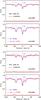 |
Fig. 2 Galactic Na i absorption toward PKS 1229−02: spectrum, its error (red curves) and simultaneous fit to both transitions (blue curve). The UVES 2002 data are shown in the top panel; in the bottom panel we display the UVES 2011 data together with the fits to the 2002 data (blue). Note the disappearance of the component at vhelio = 9.6 km s-1 (thick vertical tick mark), within a period of 9.2 yr. The heliocentric redshift z = −0.000159 (strongest component) corresponds to v = 0 km s-1. |
Towards AO 0235+164, the Galactic Na i absorption shows a strong, single component at zabs = + 0.00002. A simultaneous fit to both members of the Na i doublet yields identical values at the two epochs, 9.2 yr apart, within the 1σ errors: N(Na i) = (2.51 ± 0.04) × 1012 cm-2.
The Galactic Na i absorption towards PKS 1229−02 is multiple (5 components) and extends over 76 km s-1. Significant variation is present for the component at zabs = −0.000127: in 9.7 yr, it has nearly disappeared, with N(Na i) decreasing by a factor of four (see Table 3 and Fig. 2). The three other strong components (N(Na i) > 1011 cm-2) did not vary (1σ: 17%).
Towards PKS 1741−038, Galactic molecular absorptions at vLSR = 2 km s-1 have been extensively investigated with detections of HCO+ (Lucas & Liszt 1996), CO (Akeson & Blitz 1999), and C2H (Lucas & Liszt 2000), together with variable 21 cm absorption (Lazio et al. 2001). The associated Na i absorption at zabs = −0.00033 is multiple (4 components), partly saturated, and blended with atmospheric Na i emission, thus preventing a search for variations. Two well-known 5780 and 5797 Å DIBs are detected at both epochs. Their equivalent widths are equal to 0.33 and 0.10 Å, respectively, and are similar at two epochs 9.8 yr apart with ΔW/⟨ W⟩ = 21% ± 13% and 20% ± 23%. Two other DIBs at 4428 and 6196 Å, the Ca ii doublet and CH+λ4232, are detected but are far too noisy in the 2001 spectrum to investigate variability.
Finally, towards FBQS J2340−0053, the Na i 5897 line is not covered in the HIRES spectrum. The single component of the Ca ii doublet at zabs = −0.00002 remains stable (1σ: 3.8%) within 1.9 yr.
3.3. Neutral and molecular gas at high z
Towards PKS 0458−020, C i is well detected at zabs = 1.5605 in the HIRES spectrum (with a single component, as reported in Kanekar et al. 2010) but with too low a S/N in the UVES spectrum to get useful variability constraints. In FBQS J2340−0053 spectra, C i is detected at zabs = 1.3606 and 2.0545. The three well-separated components of the lower z system are stable (1σ: 12%). The fit of C i at zabs = 2.0545 involves a minimum of eight components, two sets being heavily blended (components 3–4 and 5–6, respectively). Within the blend at zabs = 2.05473, a very narrow component (number 6) shows a possible variation ΔN/⟨N ⟩ of 69% in 0.71 yr (rest frame) at the 3.0σ significance level (see Table 3 and Fig. 3 left panel); the 1σ limits for the other seven components are in the range 9–50%.
Molecular hydrogen has already been detected towards FBQS J2340−0053 at zabs = 2.0545 (Jorgenson et al. 2010). The Lyman and Werner transitions display six components (which roughly correspond to C i components number 1, 2, 3–4, 5–6, 7, and 8), and there is a possible variation of the sixth H2, J = 3 weak component at zabs = 2.05513. Using the unblended components of the transitions at 1081, 1084, and 1099 Å, we find a decrease, ΔN/⟨N⟩ = −34%, in only 0.71 yr (rest frame), significant at the 3.1σ level (Table 3 and Fig. 3, right panel). Unfortunately, the corresponding C i features are too weak to check whether C i lines display similar variations (in the left panel of Fig. 3, features at v ≃ 40 km s-1 for the C iλ1277 and C iλ1328 transitions are in fact dominated by C i∗ transitions from the strongest components). Conversely, the fourth H2 component, which corresponds to the second C i blend (components 5 and 6) with marginal variations is opaque in the available transitions, hence insensitive to time changes.
3.4. The Mg II–Fe II systems
3.4.1. Low β Mg II systems
There are only two blazars with low β Mg ii systems of moderate strength. For the other three, these systems are either DLAs or extremely strong saturated Mg ii absorbers. We then searched for proxies of intermediate opacity (e.g. Fe ii lines) to constrain variability.
Towards AO 0235+164, there are three Mg ii systems at low β: zabs = 0.8514 (three fitted components), 0.8523 (seven components), and 0.85562 (single). There is no variation in the triple and single systems (1σ limits on ΔN/⟨N ⟩ of 9.5% and 6.3%, respectively). For the multiple system, one Mg ii component at zabs = 0.85236, blended with two weaker ones at zabs = 0.85231 and 0.85241, shows a tentative variability of its column density ΔN/⟨N ⟩ of 53% in 5.0 yr (absorber rest frame), but at a low significance level of only 2.3σ (see Table 3 and Fig. 4). For these three components, the associated Fe ii doublet is stable (1σ: 5.2%)
Towards PKS 1229−02, there is a triple, unblended system at zabs = 0.830. The strongest component at zabs = 0.83032 shows a marginal small variation ΔN/⟨N ⟩ of 17% in 5.0 yr (rest frame) at a 3.7σ significance level (Table 3 and Fig. 5). There is no variation in the associated four strongest Fe ii lines (1σ: 7.3%). The systems at zabs = 0.83102 and 0.83128 are too weak to derive meaningful limits on their variabilty. There are two other Mg ii systems at β ≤ 0.15, and they are stable: the weak, single-component doublet at zabs = 0.7684 (1σ: 8.7%) and the triple system at zabs = 0.7564 with one nearly saturated component (1σ: 20%).
Only one of the three targets with extremely strong saturated, low β Mg ii systems has proxy lines that yield meaningful limits. Towards PKS 0458−020, the Ni ii triplet and the Zn ii-Cr ii lines at zabs = 2.03956 all have moderate strength and are heavily blended without clear variation. In PKS 1741−038 spectra, the Fe ii lines are saturated. Thus, some variability constraint can only be placed on the zabs = 2.0545 DLA absorber towards FBQS J2340−0053: the three strongest S ii components of medium strength at zabs = 2.0546 and the strongest one of Al iii at zabs = 2.05511 do not show variability (1σ: 32% and 28%, respectively; see Sect. 4.2).
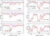 |
Fig. 3 C iλ1277,1280,1328 and molecular H2, J = 3λ1081,1084,1081 absorptions at zabs = 2.05472 towards FBQS J2340−0053 in the November 2006 (HIRES, black line) and October 2008 (UVES, red line) spectra. Left panel: the eight C i components required to fit the profiles are shown by blue ticks, and the marginally varying feature is at v = 0 (thick tick). In the top C iλ1280 plot, three C iλ1656 lines from the zabs = 1.3606 system are also shown (green ticks). For the C iλ1277 and C iλ1328 transitions, we show the position expected for C i∗ transitions associated with the 8 components (cyan ticks). The features at v ≃ 40 km s-1 are mainly due to C i∗ transitions. Right panel: six H2J = 3 components are required to fit the profiles. Marginal variability is seen in the sixth component (thick tick) at v ≃ 40 km s-1. Some difference is also seen in the fifth component, but it is significant only at the 2.0σ level, instead of 3.1σ for the sixth one. For both narrow components displaying marginal variations in C i (v ≃ 0) or H2 (v ≃ 40 km s-1), we checked that the slightly higher resolution of the HIRES spectrum cannot account for the observed difference between the profiles. |
3.4.2. High β Mg II systems
For the high β systems, variations are not detected from either their Mg ii doublets or proxy lines. Towards AO 0235+164, the two strongest components of the Ca ii doublet at zabs = 0.5239, associated with the DLA, do not vary (1σ: 26%). Towards PKS 0458−020, the Fe iiλλ2344,2382 lines at zabs = 1.5271 (selecting the 3 unblended components) do not vary either (1σ: 15%). Finally, towards FBQS J2340−0053, the highly multiple Fe ii system at zabs = 1.3606, associated with C i and 21 cm absorptions, is stable (1σ: 14% for all the components, using the weak Fe iiλλ2249, 2260 doublet to constrain the other nearly saturated lines).
4. Discussion
4.1. Presence of intrinsic systems in blazar spectra?
Time variability of narrow absorption lines at low β have been securely detected in small samples of high ionisation systems (involving C iv, N v, and O vi), observed at low and intermediate resolution (Narayanan et al. 2004; Wise et al. 2004; Hamann et al. 2011). The lines showing variations are essentially from mini-BALs and associated (Δv< 5000 km s-1) narrow-line systems. The time-scales investigated (in the quasar rest frame) range from 0.28 to 8.8 yr, and the variable narrow lines remained fixed in velocity. High and low ionization systems (at β> 0.01) with repeated observations have been identified by Hacker et al. (2013) in a very large sample of SDSS-DR7 quasar spectra: 33 out of 1084 systems have absorption lines with variations in their equivalent widths. For most of them Wr> 0.3 Å and ΔWr/Wr> 50%, with two-thirds of the variable systems being at “relatively low” β (<0.22). Low ionisation species are present in all the 33 variable systems, and C iv is detected in the 17 systems at sufficiently high zabs (>1.50). Chen et al. (2013) focussed their variability study on associated (β< 0.03) Mg ii systems identified in SDSS-DR7 and SDSS-DR9 (BOSS survey) spectra. They do not detect time variations at a significance level higher than 3σ in their sample of 36 Mg ii doublets.
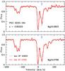 |
Fig. 4 Intervening Mg ii absorption at zabs = 0.852 towards AO 0235+164 in the 1997 December (HIRES, black line) and 2007 February (UVES, red line) spectra (lower panel: Mg iiλ2796; upper panel: Mg iiλ2803). The blue vertical tick underlines a marginally variable blended component at zabs = 0.85237, although at only a 2.3σ significance level. |
No variation of intervening Mg ii systems in high spectral resolution spectra has been reported so far. Amongst the five targets in our sample, three blazars have in total six Mg ii doublets at β ≤ 0.15 that are suitable (unsaturated, not heavily blended lines) for variability studies. As described in Sect. 3.4, only marginal column density variations have been detected for two zabs ~ 0.85 Mg ii absorbers at significance levels of 2.3σ and 3.7σ, respectively. The four other Mg ii absorbers at zabs ~ 0.75–0.85 are stable with ΔN/⟨N ⟩ in the range 6–20% at 1σ confidence level. Among them, the one in the spectrum of AO 0235+164 is 150 km s-1 away from the tentatively variable system.
In Bergeron et al. (2011), we found a potential excess of Mg ii systems at β ≈ 0.1 in blazar spectra and proposed that gas swept up by the AGN jet could be responsible for it. In such a scenario, absorption line variability can be expected, but, in the absence of predictions from numerical simulations, it is difficult to anticipate the time scale and magnitude expected for the column density changes; this should depend strongly on the occurrence of marked variations in the activity of the nucleus itself at about the time when the blazar was observed. Thus, we cannot really draw conclusions from the lack of clear evidence for time variations among the limited set of systems that we could investigate here.
4.2. Structure in moderately ionised halo gas
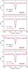 |
Fig. 5 Intervening Mg ii absorption at zabs = 0.83032 towards PKS 1229−02: spectrum and its error (red curves), together with a simultaneous fit to both transitions (blue curve). In the upper panel, we show the UVES 2002 data, while the bottom panel displays the UVES 2011 data with the fit performed on the UVES 2002 spectrum. The blue vertical tick underlines the marginally variable Mg ii doublet. |
We now discuss systems involving narrow absorption lines associated with halo gas that is optically thick to UV ionizing radiation, i.e. gas classically traced by Mg ii or Fe ii transitions. We mentioned above the few cases for which we could get stringent upper limits on column density variations for discrete velocity components seen through intermediate opacity lines. One good example is the zabs = 1.3606 system towards FBQS J2340−0053 involving 10 Fe ii components. Even when most of the absorption profile is optically thick (this is often the case for the Mg ii doublet), the data can be used to search for variations near the profile edges (e.g. appearance or disappearance of faint components). We could not identify any change of this kind. Moreover, since the component redshifts are allowed to be free when fitting the profiles, we could also get constraints on velocity variations; again, we found no significant change, with 3σ upper limits generally below 1 km s-1. Occasionally, some line profiles are observed to be rather smooth as seen for the resolved S iiλ1253 and 1259 lines at zabs = 2.05454 in the FBQS J2340−0053 spectrum. As shown in Fig. 6, no significant difference is seen along the entire profile. The 1σ upper limit on the relative flux variation is 1.7 × 10⁻² per resolution element along the S iiλ1259 line profile. Since the latter spans over 120 km s-1, the previous upper limit applies to about 120 / 6.6 ≃ 18 distinct resolution elements.
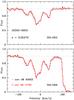 |
Fig. 6 S iiλλ1253,1259 absorption at zabs = 2.05454 towards FBQS J2340−0053 in the 2006 November (HIRES, black line) and 2008 October (UVES, red line) spectra. |
To conclude the discussion for these systems, we detected no structure in the density and velocity field within Mg ii/Fe ii halos on the scales that we could probe (typically of the order of 100 au). This is consistent with previous observations of moderately ionised gas in galaxy halos. Indeed, both Rauch et al. (2002) and Kobayashi et al. (2002) find that a typical value for the cloud size associated with the individual velocity components is 200 pc, implying very little structure on the much smaller scales that we probe here. We also note that, from the analysis of the number density of strong Mg ii systems detected on top of quasar emission lines in SDSS spectra, Lawther et al. (2012) derive a lower limit of about 0.03 pc for the individual Mg ii absorbing clouds. Finally, Welty (2007) analysed multi-epoch HST spectra of HD 219188 and detect no variations for S ii, O i, Si ii, and Fe ii in the disk of our own Galaxy, on scales of the order of 100 au. Thus, our results are in good agreement with all known constraints on structure in moderately ionised gas.
In this context, the variations tentatively detected by Hacker et al. (2013) for narrow intervening Mg ii systems are most surprising. These authors analysed more than 1000 reliable quasar absorption systems with multi-epoch observations and extracted a small subset of 33 systems displaying some evidence for time changes in their equivalent widths. Their study differs markedly from ours in the number of systems investigated, and given the small fraction of systems showing variability – about 3% – it is true that we expect very few variable lines in our sample. However, it should be stressed that the two studies also differ strongly in the sensitivity expressed in terms of ΔWr or ΔWr/Wr. The variations reported in the SDSS spectra are very large with, in most cases, ΔWr> 0.3 Å and ΔWr/Wr> 50%, corresponding to even greater fractional column density variations. For comparison, the marginal variation quoted above in the Mg iiλ2796 line at zabs = 0.83032 towards PKS 1229−02 is smaller than ΔWr = 0.01 Å and ΔWr/Wr = 5%.
If the large variations quoted by Hacker et al. (2013) are real, one can imagine that the number of systems expected to display changes at the level that we can reach in our high resolution study should be much greater, coming into contradiction with the absence of clear detection of variations in our sample. Before drawing any conclusion, additional observations aiming at confirming the status of the 33 potentially variable systems would be highly desirable. In particular, since variations are (to first order) expected to be regular, a third spectrum should confirm the trend observed on the two first ones. Such a work is currently in progress (see Appendix B2 in Dawson et al. 2013). Repeated high resolution observations of the brightest quasars involved would also be very useful for checking the reality of time variations and characterising them.
4.3. High z neutral/molecular gas
C i and H2 are known to be closely related in diffuse molecular clouds (Srianand et al. 2005). Indeed, the velocity components found for both species are generally similar, although some significant differences in their relative strength can be observed, as is the case for the zabs = 2.0545 system towards FBQS J2340−0053 (Sect. 3.3 and Fig. 3). We successively discuss these two tracers below.
C i lines are detected in three high z systems, one towards PKS 0458−020 and two towards FBQS J2340−0053, but useful constraints could be obtained only for the last two at zabs = 1.3606 (no change in N) and 2.0454 (possible variation of about 70% for an unresolved component). Unfortunately, since i) the transverse velocity of the quasar is unknown; and ii) the LoS drift is determined solely by the quasar motion for the zabs = 2.0545 system because zabs ≃ zem, it is not possible to compute the scale probed through the neutral gas. Furthermore, since the transverse observer’s velocity for this target is only 12 km s-1, little drift due to the observer’s motion is expected for the zabs = 1.3606 absorber. We can then just get a typical value for the drifts by assuming a transverse velocity of about 300 km s-1 for the intervening galaxies. This value, together with a time interval of 1.9 yr (observer’s frame) between the two observations, corresponds to a linear scale of about 50 and 40 au at zabs = 1.3606 and 2.0545, respectively. In our own Galaxy, the available information on structure in the C i distribution remains quite limited. Welty (2007) performed a detailed study of the time behaviour observed for visible and UV transitions due to an intermediate velocity cloud towards the star HD 219188. Variations by a factor of about two are seen for Na i, C i, and Ca ii column densities on scales of tens of au. Qualitatively, Na i and C i display the same time behaviour, indicating that the more extensive results obtained on the Na i structure (Crawford 2003; Smoker et al. 2011) are also probably valid for C i. In this context, results obtained for N(C i) at zabs = 1.3606 and 2.0545 are certainly consistent with the properties known for Galactic gas. Clearly, studies involving more systems are desirable to reach firm conclusions.
Regarding H2, velocity components number 5 and 6 display an intermediate opacity that provides good sensitivity for the J = 3 column densities. The other J = 3 components are either too weak or too saturated; similarly, J = 2 lines are too strong, while J = 4 are too weak to be suitable. The detection of marginal variations in component number 6 is interesting in the context of questions related to the “warm H2” observed along many Galactic LoS (Gry et al. 2002; Jensen et al. 2010). Ultraviolet pumping is generally found to be insufficient for explaining the observed excess of J ≥ 2 H2 with respect to the amount expected for a thermal distribution (Gry et al. 2002). Small structures (like shocks or turbulent vortices) where the temperature can locally reach high values have been proposed to account for both the production of species like CH+ and the relative amount of J ≥ 2 H2 (Godard et al. 2009). Presently, there are no direct constraints on the size of these putative regions.
In our Galaxy, the only repeated measurements in the far-UV were performed towards the runaway O star, HD 34078 (Boissé et al. 2009). Stringent constraints were derived from the analysis of damped line profiles associated with J = 0 lines, but no limit could be obtained for the J = 2,3,4 levels because the corresponding lines are insensitive to small relative changes in N. It is noticeable that for the varying component towards FBQS J2340−0053, the N(J = 0,1,2,3) values (1.39 × 10¹⁷, 2.61 × 10¹⁷, 4.71 × 10¹⁵ and 5.28 × 1014 cm-2; for the J = 3 column density, we give the average of the 2006 and 2008 values) are consistent with a unique excitation temperature, Tex = 120 K, unlike what is seen over most of Galactic LoS where an excitation temperature of about 300 K is required to fit N(J) values at J ≥ 2 (Jensen et al. 2010). This indicates that the gas is dense enough to ensure thermalisation, which is in qualitative agreement with the small size suggested by the time variations observed for this component.
4.4. Local Galactic gas
We found a large variation (factor of four) in Galatic N(Na i) for one of the five velocity components towards PKS 1229−02. The constraint on the corresponding cloudlet size can be estimated from the peculiar motion of the Sun with respect to the LSR (see Sect. 2.2). For this direction, the Sun’s velocity is mostly transverse with Vt (Sun)/LSR = 17.8 km s-1, implying a drift of about 35 au. This is well within the range (typically a few 10 au or larger) for which Na i line changes have been observed on other LoS (Crawford 2003). The other four components towards PKS 1229−02 remained stable on the same linear scale, indicating that the associated fragments are characterised by sizes larger than 100 au. For other targets providing useful constraints on Galactic gas structure, we find variation neither towards AO 0235+164 nor towards FBQS J2340−0053. The transverse velocity of the Sun for these two targets is 15.8 km s-1 and 16.6 km s-1, respectively, implying drifts of about 30 and 7 au in local material. In these two cases, Na i lines have a relatively high opacity, implying a poor sensitivity to variations.
Towards PKS 1741−038, the estimated drift over the 9.8 yr separating the two observations is about 17 au. The absence of variations in DIBs near 5780.5 and 5797.1 Å can be related to results obtained recently by Cordiner et al. (2013) for ρ Oph stars. These authors find variations of about 5–9% for the above DIBs on scales exceeding 300 au. Thus, given our limited sensitivity, the observed stability is not surprising.
5. Summary and prospects for further studies
As discussed above, the only clear and unambiguous variation has been detected for the Na i doublet from our own Galaxy towards PKS 1229−02, in good agreement with previous results on the au-scale structure of neutral Galactic gas. In the same kind of media but at higher redshifts (z ≈ 2 toward FBQS J2340−0053), we also find tentative evidence of structure in neutral and molecular gas: C i with ΔN/⟨N ⟩ ≃ 70% at the 3.0σ significance level and H2 with ΔN/⟨N⟩ ≃ 35% at the 3.1σ level. For low β absorption systems in blazar spectra, absorption profiles are, for the most part, very stable and only a marginal 3.7σ 17% variation has been seen in the strength of a narrow Mg ii component towards PKS 1229−02. On the other hand, no change was seen for moderately ionised gas at high β (i.e. intervening halo gas), which again is consistent with known constraints on typical cloud sizes in such media.
The results discussed above illustrate well the potential and the limits of the method used in this paper to investigate the small-scale structure of absorbing gas in quasar spectra. We first outline the high value of high spectral resolution. Often, several transitions from the same species are detected and can be used to fit absorption line profiles, thus yielding well constrained b and N values for the velocity components seen at each epoch. This redundancy provides a powerful objective way (at least for those components that are partially resolved) to assess the reality of time changes and rule out false variations. Indeed, it is very unlikely to find two artefacts mimicking true variations by chance, i.e. occurring on two line profiles at the same position in velocity space and with a strength consistent with the f values of the transitions involved. If species displaying more than two transitions (like C i or H2) can be used to increase the redundancy and the range covered by f values, the probability is even lower, and better constraints can be derived from line fitting. Conversely, the Mg ii system at zabs = 0.85236 towards AO 0235+164 illustrates well that with only two transitions differing in their f values by a factor no higher than two, one may be unable to reach firm conclusions when variations are moderate. Furthermore, high resolution allows us to quantify the changes in meaningful astrophysical parameters, N and b values, or to set upper bounds on their variations. Limitations appear, however, for some line profiles (e.g. the C i component towards FBQS J2340−0053 for which variations are suspected), when the decomposition into discrete components required by line fitting is poorly defined or not unique. Such difficulties mean that the spectral resolution used is not high enough to analyse the velocity distribution properly, implying that line opacities, as well as N and b values, cannot be determined reliably. One should therefore prefer absorption systems with simple velocity structure for repeated observations.
Our study considered several topics for which useful constraints can be obtained from an investigation of time variations. We now discuss prospects for two of them. We mentioned above that, generally, we have poor knowledge of the scales probed by repeat observations because the transverse motion of the target is not measurable. The situation is more favourable for low redshift absorbers because the drift of the LoS through the intervening gas is determined mainly by the observer’s motion, which is inferred directly from observations of the CMB dipole. For instance, to study whether the small-scale structure seen in the Galactic neutral or weakly ionised gas is ubiquitous in external galaxies, one could observe quasars belonging to the so-called quasar-galaxy pairs again (see e.g. Bowen et al. 1991) and search for temporal changes in the Ca ii or Na i lines over more than 20 yr. Of course, targets located in directions that are more or less normal to our large-scale peculiar velocity should be preferred (in this favourable configuration, the scales probed over 20 yr are of the order of 1500 au). Regarding high redshift absorbers, for which only a rough estimate of the scales probed can be obtained, one needs to observe a statistically significant sample of targets to derive meaningful results concerning the presence and strength of small-scale structure. Some quasars are found in pairs (Hennawi et al. 2010), and occasionally, absorbers appear to belong to galaxy clusters (Whiting et al. 2006), implying increased peculiar velocities. Such LoS will, on average, be associated with larger drifts, and should be targetted preferentially.
A second topic for which repeated observations of quasars at high spectral resolution are especially timely involves the properties and origin of the warm (J ≥ 2) H2 found in diffuse molecular gas in our own Galaxy, as well as in high redshift absorbers. During the past ten years, the number of high z H2 systems has increased very significantly and now exceeds 20 (Albornoz-Vásquez et al. 2014). Some of them display narrow velocity components that are well suited to a detailed study (see e.g. Noterdaeme et al. 2007). As discussed in Sect. 3 for the system at zabs = 2.0545 towards FBQS J2340−0053, multi-epoch observations can provide key information on the typical size of regions where diffuse molecular gas is heated to temperatures above 200 K. Such high z warm H2 is seen at epochs when star formation was much more efficient than today (Madau & Dickinson 2014), and one can therefore anticipate that the diffuse molecular medium should be strongly affected by a very high dissipation rate of the mechanical energy carried by shock waves and turbulence.
To conclude, we wish to stress that the data used here were acquired for purposes other than variability searches and thus are certainly not the best choice for our study. First, the two spectra available for each target often differ significantly in their S/N, and one is then limited in the comparison by the lower quality spectrum. The time interval also varies a lot from target to target and, unfortunately, the lag for the quasar displaying the richest spectrum – FBQS J2340−0053 – is of only two years. A straightforward strategy for getting better constraints or addressing some of the questions discussed above with more appropriate data would consist in i) selecting targets that display the required types of absorption lines and targets with one already available good high resolution spectrum taken at least ten years ago; and ii) observing them again at similar S/N and resolution. Obviously, the existence of databases where high resolution quasar spectra are archived properly are extremely useful in such an approach. Finally, we note that improvements in the accuracy of wavelength calibrations accomplished recently in the context of the ESO Large Programme designed to constrain the variation in fundamental constants (Molaro et al. 2013) or improvements foreseen for instruments that will become available in the near future (e.g. the ESPRESSO spectrograph to be mounted on the ESO/VLT telescope) should indeed help to investigate the velocity field within the absorbers in more detail.
Acknowledgments
We are very grateful to several colleagues who provided some of the spectra used in our study or contributed to their reduction: John Black (for the 2001 PKS 1741-038 spectrum), Cédric Ledoux (PKS 0458-020, UVES data), Pasquier Noterdaeme and Hadi Rahmani (FBQS J2340-0053, UVES data), John O’Meara (AO 0235+164, HIRES spectrum), and Giovanni Vladilo (UVES spectra of AO 0235+164 and PKS 1229-02). Thanks are also due to Jean-Philippe Uzan for discussions about the estimate of line-of-sight drifts on cosmological scales and to Gary Mamon for help on data handling techniques. We are grateful to the referee for several constructive comments that helped to clarify the content of this paper.
References
- Akeson, R. L., & Blitz, L. 1999, ApJ, 523, 163 [NASA ADS] [CrossRef] [Google Scholar]
- Albornoz-Vàsquez, D., Rahmani, H., Noterdaeme, P., et al. 2014, A&A, 562, A88 [NASA ADS] [CrossRef] [EDP Sciences] [Google Scholar]
- Bergeron, J., Petitjean, P., Aracil, B. et al. 2004, The Messenger, 118, 40 [NASA ADS] [Google Scholar]
- Bergeron, J., Boissé, P., & Ménard, B. 2011, A&A, 525, A51 [NASA ADS] [CrossRef] [EDP Sciences] [Google Scholar]
- Boissé, P., Rollinde, E., Hily-Blant, P., et al. 2009, A&A, 501, 221 [NASA ADS] [CrossRef] [EDP Sciences] [Google Scholar]
- Boissé, P., Federman, S. R., Pineau Des Forêts, G., & Ritchey, A. M. 2013, A&A, 559, A131 [NASA ADS] [CrossRef] [EDP Sciences] [Google Scholar]
- Bowen, D. V., Pettini, M., Penston, M. V., & Blades, C. 1991, MNRAS, 249, 145 [NASA ADS] [CrossRef] [Google Scholar]
- Burbidge, E. M., Beaver, E. A., Cohen, R. D., Junkkarinen, V. T., & Lyons, R. W. 1996, AJ, 112, 2533 [NASA ADS] [CrossRef] [Google Scholar]
- Chen, Z.-F., Pan, C.-J., Li, G.-Q., Huang, W.-R., & Li, M.-S. 2013, JA&A, 34, 317 [NASA ADS] [Google Scholar]
- Churchill, C. W., & Charlton, J. C. 1999, AJ, 118, 59 [NASA ADS] [CrossRef] [Google Scholar]
- Cordiner, M. A., Fossey, S. J., Smith, A. M., & Sarre, P. J. 2013, ApJ, 764, 10 [Google Scholar]
- Crawford, I. A. 2003, Ap&SS, 285, 661 [NASA ADS] [CrossRef] [Google Scholar]
- Crighton, N. H. M., Hennawi, J. F., Simcoe, R. A., et al. 2015, MNRAS, 446, 18 [NASA ADS] [CrossRef] [Google Scholar]
- Dai, X., Kochanek, C. S., Chartas, G., et al. 2010, ApJ, 709, 278 [NASA ADS] [CrossRef] [Google Scholar]
- Dawson, K. S., Schlegel, D. J., Ahn, C. P., et al. 2013, AJ, 145, 10 [Google Scholar]
- Filiz, A.k. N., Brandt, W. N., Hall, P. B., et al. 2013, MNRAS, 777, 168 [Google Scholar]
- Fixsen, D. J., Cheng, E. S., Gales, J. M., et al. 1996, ApJ, 473, 576 [NASA ADS] [CrossRef] [Google Scholar]
- Godard, B., Falgarone, E., & Pineau Des Forêts, G. 2009, A&A, 495, 847 [NASA ADS] [CrossRef] [EDP Sciences] [Google Scholar]
- Grier, C. J., Hall, P. B., Brandt, W. N., et al. 2015, ApJ, 806, 111 [NASA ADS] [CrossRef] [Google Scholar]
- Gry, C., Boulanger, F., Nehmé, C., et al. 2002, A&A, 391, 675 [NASA ADS] [CrossRef] [EDP Sciences] [Google Scholar]
- Hacker, T. L., Brunner, R. J., Lundgren, B. F., & York, D. G. 2013, MNRAS, 434, 183 [NASA ADS] [CrossRef] [Google Scholar]
- Hennawi, J. F., Myers, A. D., Shen, Y., et al. 2010, ApJ, 719, 1672 [NASA ADS] [CrossRef] [Google Scholar]
- Hamann, F., Kaplan, K. F., Rodriguez Hidalgo, P., Prochaska, J. X., & Herbert-Fort, S. 2008, MNRAS, 391, L39 [NASA ADS] [CrossRef] [Google Scholar]
- Hamann, F., Kanekar, N., Prochaska, J. X., et al. 2011, MNRAS, 410, 1957 [NASA ADS] [Google Scholar]
- Jensen, A. G., Snow, T. P., Sonneborn, G., & Rachford, B. L. 2010, ApJ, 711, 1236 [NASA ADS] [CrossRef] [Google Scholar]
- Jorgenson, R. A., Wolfe, A. M., & Prochaska, J. X. 2010, ApJ, 723, 460 [NASA ADS] [CrossRef] [Google Scholar]
- Kanekar, N., & Chengalur, J. N. 2001, MNRAS, 325, 631 [NASA ADS] [CrossRef] [Google Scholar]
- Kanekar, N., Prochaska, J. X., Ellison, S. L., & Chengalur, J. N. 2010, ApJ, 712, L152 [NASA ADS] [CrossRef] [Google Scholar]
- Kanekar, N., Prochaska, J. X., Smette, A., et al. 2014, MNRAS, 438, 2131 [NASA ADS] [CrossRef] [Google Scholar]
- Kobayashi, N., Terada, H., Goto, M., & Tokunaga, A. 2002, ApJ, 569, 676 [NASA ADS] [CrossRef] [Google Scholar]
- Lauroesch, J. T. 2007, ASP Conf. Ser., 365, 40 [NASA ADS] [Google Scholar]
- Lawther, D., Paarup, T., Schmidt, M., et al. 2012, A&A, 546, A67 [NASA ADS] [CrossRef] [EDP Sciences] [Google Scholar]
- Lazio, T. J. W., Gaume, R. A., Claussen, M. J., et al. 2001, ApJ, 546, 267 [NASA ADS] [CrossRef] [Google Scholar]
- Le Brun, V., Bergeron, J., Boissé, P., & Deharveng, J. M. 1997, A&A, 321, 733 [NASA ADS] [Google Scholar]
- Lucas, R., & Liszt, H. 1996, A&A, 307, 252 [Google Scholar]
- Lucas, R., & Liszt, H. 2000, A&A, 358, 1069 [NASA ADS] [Google Scholar]
- Madau, P., & Dickinson, M. 2014, ARA&A, 52, 415 [NASA ADS] [CrossRef] [Google Scholar]
- Meyer, D. M., Peek, J. E. G., Peek, J. E. G., & Heiles, C. 2012, ApJ, 752, 119 [NASA ADS] [CrossRef] [Google Scholar]
- Misawa, T., Charlton, J. C., & Eracleous, M. 2014, ApJ, 792, 77 [NASA ADS] [CrossRef] [Google Scholar]
- Molaro, P., Centurión, M., Whitmore, J. B., et al. 2013, A&A, 555, A68 [NASA ADS] [CrossRef] [EDP Sciences] [Google Scholar]
- Narayanan, D., Hamann, F., Barlow, T., et al. 2004, ApJ, 601, 715 [NASA ADS] [CrossRef] [Google Scholar]
- Neeleman, M., Prochaska, J. X., & Wolfe, A. M. 2015, ApJ, 800, 7 [Google Scholar]
- Noterdaeme, P., Ledoux, C., Petitjean, P., et al. 2007, A&A, 474, 393 [Google Scholar]
- Rahmani, H., Srianand, R., Gupta, N., et al. 2012, MNRAS, 425, 556 [NASA ADS] [CrossRef] [Google Scholar]
- Rauch, M., Sargent, W. L. W., Barlow, T. A., & Simcoe, R. A. 2002, ApJ, 576, 45 [NASA ADS] [CrossRef] [Google Scholar]
- Savage, B. D., & Sembach, K. R. 1991, ApJ, 379, 245 [NASA ADS] [CrossRef] [Google Scholar]
- Srianand, R., Petitjean, P., Ledoux, C., Ferland, G., & Shaw, G. 2005, MNRAS, 362, 549 [Google Scholar]
- Smoker, J. V., Bagnulo, S., Cabanac, R., et al. 2011, MNRAS, 414, 59 [NASA ADS] [CrossRef] [Google Scholar]
- Welty, D. E. 2007, ApJ, 668, 1012 [NASA ADS] [CrossRef] [Google Scholar]
- Whiting, M. T., Webster, R. L., & Francis, P. J. 2006, MNRAS, 368, 341 [NASA ADS] [CrossRef] [Google Scholar]
- Wise, J. H., Eracleous, M., Charlton, J. C., & Ganguly, R. 2004, ApJ, 613, 129 [NASA ADS] [CrossRef] [Google Scholar]
- Wolfe, A. M., Davis, M. M., & Briggs, F. H. 1982, ApJ, 259, 495 [NASA ADS] [CrossRef] [Google Scholar]
All Tables
All Figures
|
Fig. 1 Observer and target move with 3D velocities VO and VT in the cosmological frame. Their transverse component VO ⊥ and VT ⊥ determines the transverse velocity VM ⊥ of the impact point M. The latter combines with the transverse velocity of the absorber VA ⊥ to define the relative drift velocity of the LoS with respect to the gas, Vd, which sets the scale probed within the absorber during a given time interval. |
| In the text | |
|
Fig. 2 Galactic Na i absorption toward PKS 1229−02: spectrum, its error (red curves) and simultaneous fit to both transitions (blue curve). The UVES 2002 data are shown in the top panel; in the bottom panel we display the UVES 2011 data together with the fits to the 2002 data (blue). Note the disappearance of the component at vhelio = 9.6 km s-1 (thick vertical tick mark), within a period of 9.2 yr. The heliocentric redshift z = −0.000159 (strongest component) corresponds to v = 0 km s-1. |
| In the text | |
|
Fig. 3 C iλ1277,1280,1328 and molecular H2, J = 3λ1081,1084,1081 absorptions at zabs = 2.05472 towards FBQS J2340−0053 in the November 2006 (HIRES, black line) and October 2008 (UVES, red line) spectra. Left panel: the eight C i components required to fit the profiles are shown by blue ticks, and the marginally varying feature is at v = 0 (thick tick). In the top C iλ1280 plot, three C iλ1656 lines from the zabs = 1.3606 system are also shown (green ticks). For the C iλ1277 and C iλ1328 transitions, we show the position expected for C i∗ transitions associated with the 8 components (cyan ticks). The features at v ≃ 40 km s-1 are mainly due to C i∗ transitions. Right panel: six H2J = 3 components are required to fit the profiles. Marginal variability is seen in the sixth component (thick tick) at v ≃ 40 km s-1. Some difference is also seen in the fifth component, but it is significant only at the 2.0σ level, instead of 3.1σ for the sixth one. For both narrow components displaying marginal variations in C i (v ≃ 0) or H2 (v ≃ 40 km s-1), we checked that the slightly higher resolution of the HIRES spectrum cannot account for the observed difference between the profiles. |
| In the text | |
|
Fig. 4 Intervening Mg ii absorption at zabs = 0.852 towards AO 0235+164 in the 1997 December (HIRES, black line) and 2007 February (UVES, red line) spectra (lower panel: Mg iiλ2796; upper panel: Mg iiλ2803). The blue vertical tick underlines a marginally variable blended component at zabs = 0.85237, although at only a 2.3σ significance level. |
| In the text | |
|
Fig. 5 Intervening Mg ii absorption at zabs = 0.83032 towards PKS 1229−02: spectrum and its error (red curves), together with a simultaneous fit to both transitions (blue curve). In the upper panel, we show the UVES 2002 data, while the bottom panel displays the UVES 2011 data with the fit performed on the UVES 2002 spectrum. The blue vertical tick underlines the marginally variable Mg ii doublet. |
| In the text | |
|
Fig. 6 S iiλλ1253,1259 absorption at zabs = 2.05454 towards FBQS J2340−0053 in the 2006 November (HIRES, black line) and 2008 October (UVES, red line) spectra. |
| In the text | |
Current usage metrics show cumulative count of Article Views (full-text article views including HTML views, PDF and ePub downloads, according to the available data) and Abstracts Views on Vision4Press platform.
Data correspond to usage on the plateform after 2015. The current usage metrics is available 48-96 hours after online publication and is updated daily on week days.
Initial download of the metrics may take a while.