| Issue |
A&A
Volume 581, September 2015
|
|
|---|---|---|
| Article Number | A10 | |
| Number of page(s) | 35 | |
| Section | Extragalactic astronomy | |
| DOI | https://doi.org/10.1051/0004-6361/201526252 | |
| Published online | 24 August 2015 | |
VEGAS: A VST Early-type GAlaxy Survey
I. Presentation, wide-field surface photometry, and substructures in NGC 4472⋆
1 INAF–Astronomical Observatory of Capodimonte, Salita Moiariello 16, 80131 Naples, Italy
e-mail: This email address is being protected from spambots. You need JavaScript enabled to view it.
2 University of Naples Federico II, C.U. Monte Sant’Angelo, via Cinthia, 80126 Naples, Italy
3 INAF–Astronomical Observatory of Teramo, via Maggini, 64100 Teramo, Italy
4 Department of Physics and Astronomy, San José State University, One Washington Square, San José, CA 95192, USA
5 University of California Observatories, 1156 High Street, Santa Cruz, CA 95064, USA
6 Centre for Astrophysics & Supercomputing, Swinburne University, Hawthorn, VIC 3122, Australia
7 Institute of Astrophysics, 782-0436 Macul, Santiago, Chile
8 National Research Council Canada, Victoria, BC V9E 2E7, Canada
Received: 2 April 2015
Accepted: 15 June 2015
Abstract
Context. We present the VST Early-type GAlaxy Survey (VEGAS), which is designed to obtain deep multiband photometry in g,r,i, of about one hundred nearby galaxies down to 27.3, 26.8, and 26 mag/arcsec2 respectively, using the ESO facility VST/OmegaCAM.
Aims. The goals of the survey are 1) to map the light distribution up to ten effective radii, re; 2) to trace color gradients and surface brightness fluctuation gradients out to a few re for stellar population characterization; and 3) to obtain a full census of the satellite systems (globular clusters and dwarf galaxies) out to 20% of the galaxy virial radius. The external regions of galaxies retain signatures of the formation and evolution mechanisms that shaped them, and the study of nearby objects enables a detailed analysis of their morphology and interaction features. To clarify the complex variety of formation mechanisms of early-type galaxies (ETGs), wide and deep photometry is the primary observational step, which at the moment has been pursued with only a few dedicated programs. The VEGAS survey has been designated to provide these data for a volume-limited sample with exceptional image quality.
Methods. In this commissioning photometric paper we illustrate the capabilities of the survey using g- and i-band VST/OmegaCAM images of the nearby galaxy NGC 4472 and of smaller ETGs in the surrounding field.
Results. Our surface brightness profiles reach rather faint levels and agree excellently well with previous literature. Genuine new results concern the detection of an intracluster light tail in NGC 4472 and of various substructures at increasing scales. We have also produced extended (g − i) color profiles.
Conclusions. The VST/OmegaCAM data that we acquire in the context of the VEGAS survey provide a detailed view of substructures in the optical emission from extended galaxies, which can be as faint as a hundred times below the sky level.
Key words: techniques: image processing / galaxies: elliptical and lenticular, cD / gravitation / galaxies: fundamental parameters / galaxies: formation
Appendices are available in electronic form at http://www.aanda.org
© ESO, 2015
1. Introduction
Recent years have witnessed renewed interest in bright early-type galaxies (ETGs). Observations at high redshift revealed that ETGs have undergone remarkable amounts of size evolution over time (e.g., Daddi et al. 2005; van Dokkum et al. 2010). Theory suggests this growth to be a basic aspect of hierarchical structure formation, with mergers building up extended bulges and stellar halos (Oser et al. 2010; Hopkins et al. 2010).
The new paradigm of “two-phase” or “inside-out” galaxy assembly, pictured by cosmological simulations, outlines two regimes in the formation of the baryonic structure of a galaxy. In a first early (z ≳ 2) phase there is rapid in situ star formation from infalling cold gas, followed by a longer accretion phase where the system considerably grows in size and mass by accreting smaller satellites. This new paradigm motivates a return to classical studies of nearby ETGs, searching for the expected signatures of formational processes, particularly at large radii.
Pilot studies have indeed revealed extensive evidence of outer galaxy assembly: from pervasive photometric substructures (Tal et al. 2009; Janowiecki et al. 2010) to metallicity gradients (Coccato et al. 2010; Forbes et al. 2011), rotational changes (Proctor et al. 2009; Coccato et al. 2009; Arnold et al. 2011), and accretion signatures in chemo-dynamical phase space (Romanowsky et al. 2012).
A full understanding of any galaxy begins with photometry. The situation for nearby ETGs is the following: the central regions are studied in much detail (e.g., Ferrarese et al. 2006, hereafter F+06; Côté et al. 2007), while the faint outskirts are still poorly investigated, even if they are becoming a hot topic with multiple surveys being carried out (e.g., Kormendy et al. 2009, hereafter K+09; Duc et al. 2015). There is a critical need for modern, wide-field (WF), multiband CCD photometry of a large sample of galaxies in a broad range of environments, replacing the photographic and narrow-field CCD work of decades past (e.g., Peletier et al. 1990; Caon et al. 1994). The aim is to systematically gauge the basic global properties of ETGs over a wide baseline of sizes: luminosity profiles, isophote shapes, substructure characteristics, color gradients, surface brightness fluctuations, inventories of satellite galaxies and globular clusters (GCs), etc. The wide range of science results and applications available from such a dataset, beyond the general goal of testing two-phase assembly models, cannot be covered here, therefore we briefly highlight a few topics.
Multiband surface brightness (SB) mapping of ETGs allows us to measure key physical parameters through the fit of generalized R1 /n profiles (Caon et al. 1993): total luminosity, Sersic index n, effective surface brightness and radius, μe and Re, boxy- or diskyness, etc. (Caon et al. 1993; Balcells et al. 2007). The correlations between them, such as μe vs. Re, mass vs. size or photometric plane (Kormendy 1985; Capaccioli et al. 1992; Shen et al. 2003) help shedding light into formation processes. Along the same line, outer breaks in the SB profiles might correlate in a non-trivial way with the inner core or cusp transition (e.g., Côté et al. 2007); this has not been studied so far. Moreover, photometry is a way to identify and gauge substructure and/or light excesses as expected from the diffuse stellar components (e.g., Zibetti et al. 2005), especially in the intracluster environment (Mihos et al. 2005, 2013), through deviations from the regular R1 /n behavior. Radial color gradients are critically related to the formation mechanisms (Carlberg 1984) because they give a hint of the different distributions in stellar ages and metallicities (Saglia et al. 2002; Pipino et al. 2008; Tortora et al. 2011). The combination of color distribution with surface brightness fluctuations (SBF, Tonry & Schneider 1988) supplies further information on the chemical properties of the stellar populations and helps lift the age-metallicity degeneracy out to a few effective radii (Cantiello et al. 2013).
 |
Fig. 1 VEGAS potential target distribution in the parameter space (blue points). Higher priority is given to galaxies with HST data (red circles) and Chandra/XMM data (yellow dots). We note that close systems are observed in a single VST/OmegaCAM pointing in many cases. |
Furthermore, accurate photometry up to 10 Re is mandatory (and still lacking) for dark matter studies because of the advent of efficient kinematical tracers such as the planetary nebulae (PNe, e.g., Romanowsky et al. 2003; Napolitano et al. 2009) and globular clusters (GCs, e.g., Romanowsky et al. 2009; Napolitano et al. 2014). In particular, extended deep photometric mapping will naturally provide a fairly complete census of galaxy satellites, from globular clusters (GCs) to satellite galaxies: a multipurpose database that is also useful for testing the formation scenarios.
Among the key questions that still remain open there is the well-known bimodality of the color distribution of GCs in galaxies (e.g., Peng et al. 2006). This has different possible explanations: i) either high-redshift, two-phase formation of elliptical systems (e.g., Forbes et al. 1997); ii) the dissipative merging of late-type spirals (e.g., Ashman & Zepf 1992); iii) the hierarchical feeding of a bright (metal-rich) elliptical by (metal-poorer) dwarfs (e.g., Côté et al. 1998); iv) the recent proposal of a unimodal metallicity distribution that is transformed into a bimodal color distribution because of the nonlinearity of color-metallicity relations (e.g., Yoon et al. 2006; Cantiello et al. 2015, and references therein). Although a unique consensus on the interpretation of this phenomenon is still lacking, we note that as in the Milky Way GC system, the systems of several other early-type galaxies are clearly bimodal in metallicity (Brodie et al. 2012, 2014; Usher et al. 2012, 2015).
Finally, satellite galaxies are important because they can be tidally disrupted in their journey around larger systems. These events are possibly the mechanisms producing the diffuse halos around galaxies (Ibata et al. 1994; Zibetti et al. 2004; Arnaboldi et al. 2012) or even the intragroup or cluster light (Mihos et al. 2013; Zibetti et al. 2005).
In view of all this and considering the special characteristics of the VLT Survey Telescope (VST; Capaccioli & Schipani 2011), a project for a photometric survey of nearby ETGs, dubbed VEGAS, has been undertaken on the Italian Guaranteed Time Observation (GTO). This is the first paper of a series where we present the survey project and its strategy, the data reduction and analysis techniques, and report on a test case conducted to assess and certify the quality of our products.
The paper is organized as follows. In Sect. 2 we briefly describe the VEGAS survey aims and objectives. The observations of a test galaxy are described in Sect. 3. In Sect. 4 we illustrate the strategies adopted for the data analysis, with a particular emphasis on the determination of the sky background and the measurement of accurate surface brightness profiles. In Sect. 5 we discuss the surface brightness profiles of the objects in this study and compare results with previous literature, while in Sect. 6 we discuss the effects of the scattered light on the surface brightness profiles. Finally, in Sect. 7 we discuss that the VST/OmegaCAM data are of the highest quality for wide-field imaging and why we believe that this machinery is a powerful tool for an “industrial” analysis of optical photometry of nearby galaxies. In Appendix A and B we describe the details of the data reduction and of the point spread function.
We adopt a distance modulus for the Virgo cluster of 31.14 ± 0.05 mag as in Mei et al. (2007). This correspond to a distance of 16.9 Mpc, so 1 arcsec is 81.9 pc. The magnitudes throughout the paper are in the AB system. Our surface brightness data are not corrected for Galactic extinction, but the total magnitude values listed in Table 1 have been corrected assuming the recipe of Arrigoni Battaia et al. (2012).
2. VEGAS survey
The VST Elliptical GAlaxies Survey (VEGAS) is a deep multiband (g,r,i) imaging survey of early-type galaxies in the southern hemisphere carried out with VST at the ESO Cerro Paranal Observatory (Chile). The large field of view (FOV) of the OmegaCAM mounted on VST (one square degree matched by pixels 0.21 arcsec wide), together with its high efficiency and spatial resolution (typically better than 1 arcsec; Kuijken 2011) allows us to map with a reasonable integration time the surface brightness of a galaxy out to isophotes encircling about 95% of the total light. Observations started in October 2011 (ESO Period 88), and since then, the survey has acquired exposures for about 20 bright galaxies (and for a wealth of companion objects in the field), for a totality of ~80 h (up to Period 93).
Since the OmegaCAM detector is a mosaic of 32 CCDs, a dithering strategy has to be devised to fill the blind gaps among the 2000 × 4000 pixels of individual CCDs. The actual implementation of the dithering strategy has consequences for setting the weight map of the various pixels of the final combined image, as well as for mixing and averaging the residual errors in the engineering of the individual CCDs because of the overlapping of adjacent CCDs.
The survey project is designed to map the surface brightness of galaxies with Ttype< 0, σ> 150, Dec < + 5, Vrad< 4000 km s-1, and Btot< − 19.2, sampling all environmental conditions and the whole parameter space. To this end, we selected from the catalog of nearby galaxies by Prugniel & Simien (1996) a large sample of about 240 potential E/S0 targets (Fig. 1) with the aim of optimizing the observing strategy throughout the year so as to observe half of this sample in five years and to uniformly cover the galaxy parameter space.
The distribution of parameters in Fig. 1 refers to the central targets of the VEGAS pointings, while we expect to simultaneously observe many lower luminosity systems. Higher priority is given to galaxies with ancillary data (e.g., HST or Chandra/XMM, see Fig. 1).
The expected depths at a signal-to-noise ratio (S/N) of >3 in the g, r, and i bands are 27.3, 26.8, and 26 mag arcsec-2, respectively. They are the result of a compromise between a reasonable exposure time and the need to detect signatures of a diffuse stellar component around galaxies (see, e.g., Zibetti et al. 2005) and the dynamical interaction of ETGs with the intergalactic medium.
The main products of the VEGAS survey are 1) a 2D light distribution out to 8–10 Re: galaxy structural parameters and diffuse light component, inner substructures as a signature of recent cannibalism events, inner disks and bars fueling active nuclei present in almost all the objects of our sample; 2) radially averaged surface brightness profiles and isophote shapes out to 10 Re; 3) color gradients and the connection with galaxy formation theories; 4) detection of external low-surface brightness structures of the galaxies and the connection with the environment; 5) census of small stellar systems (SSS: GCs, ultra-compact dwarfs and galaxy satellites) out to ~20 Re from the main galaxy center, and their photometric properties (e.g., GC luminosity function and colors, and their radial changes out to several Re), allowing us to study the properties of GCs in the outermost “fossil” regions of the host galaxy. This latter subproject is also called VEGAS-SSS (Cantiello et al. 2015). We note that the majority of studies on the photometric properties of the GC system in ETGs cover the central (few arcmin) region of the host galaxy (e.g., ACS Virgo & Fornax cluster surveys, Côté et al. 2004 and Jordán et al. 2007). An exception to the inner imaging studies is the SLUGGS survey that uses the Subaru/Suprime camera (e.g., Blom et al. 2012).
As a natural byproduct of the survey (for the depth and high S/N in the central galaxy regions), a galaxy SBF, and a SBF-gradient analysis is planned to chemically characterize the stellar population within ~2Re (or more, for the nearest ETGs in the sample).
A fundamental aspect of the survey resides in the legacy value of the data-set for ETGs, to be used for a wide range of research lines. The survey area extends from −70 to +5 degrees in Dec and 0–24 h in RA (see Fig. 1), which ensures observability throughout the year and an advantageous overlap with the KiDS survey area (de Jong et al. 2013).
VEGAS will provide a volume-limited survey in the South complementary to the Next Generation Virgo Cluster Survey (NGVS, Ferrarese et al. 2012), with similar depth but no environmental restrictions, and will be the southern equivalent to MATLAS (Duc et al. 2015)1.
3. NGC 4472 field: observations and data reduction
This first VEGAS paper presents a deep photometric analysis of the ETGs in the VST field of the galaxy NGC 4472 (M 49), the brightest member of the Virgo cluster (Table 1). We have chosen this field for the following reasons:
-
it is well-studied with an ample sci-entific photometric literature (Kimet al. 2000; Ferrareseet al. 2006; Kormendyet al. 2009; Janowieckiet al. 2010; Mihoset al. 2013);
-
it offers a wide range of cases for investigating the ability of VEGAS to map the faint galaxy outskirts. Together with this supergiant nearby object that fills almost the entire OmegaCAM field, there are smaller ETGs either embedded in the light of NGC 4472 or close to the edges of the frame (see Fig. 2). Each one of these cases requires a different data reduction strategy and calls for an independent verification.
 |
Fig. 2 VST color composite image of the 0.9° × 0.8° field around the giant galaxy NGC 4472 from g and i band VEGAS images. Circles mark the other four ETGs studied in this paper and the interacting system UGC 7636. |
Parameters of NGC 4472.
The data used in this paper consist of exposures in g and i SDSS bands (Table 2) obtained with VST + OmegaCAM in service mode under photometric sky conditions and with the following constraints:
-
S/N ≥ 3 per arcsec2;
-
dark time;
-
seeing ≤1′′;
-
airmass ≤1.2.
For the sake of clarity, we repeat that the FOV of each frame covers one square degree, with a scale of 0.21 arcsec pixel-1. The total integration time is 5695 s in g and 4590 s in i. The different exposures have the same center, which has been chosen not to coincide with that of NGC 4472, principally in order to move the galaxy core out of the central crossing of the gaps. More details about the dithering strategy can be found in the VST manual2.
VST exposures used in the photometry of the NGC 4472 field.
The data were processed with a pipeline specialized for the VST-OmegaCAM observations (dubbed VST-tube; Grado et al. 2012), which performs the following main steps:
-
prereduction;
-
astrometric and photometric calibration;
-
mosaic production.
Science images are first treated to remove the instrumental signatures, applying overscan, bias, and flat-field corrections, as well as gain harmonization of the 32 CCDs, illumination correction and, for the i band, defringing. Relative and absolute astrometric and photometric calibrations are applied before creating the final coadded image mosaics. In Appendix A we describe the various steps of the procedure in detail.
4. NGC 4472 field: photometric processing
4.1. Sky background subtraction
The background estimate and subtraction is the most critical operation in deep photometric analysis because it affects the ability of detecting and measuring the faint outskirts of galaxies.
There are at least two ways to model the sky background. The first one, extensively tested in classical photographic surface photometry (Capaccioli 1988), consists of fitting a surface, typically a 2D polynomial, to the pixel values of the mosaic that is unaffected by celestial sources or defects. The advantage comes from the simultaneity of the exposure of the galaxy and the background, which is particularly relevant in wide-field images owing to the differential effects of refraction and to the moon light, if any. Minor glitches in the CCDs’ sensitivity are averaged as well. The second method mimics the ON-OFF procedure devised in IR astronomy that is made possible by the use of digital detectors. The background is estimated from exposures taken as close as possible, in space and time, to the scientific ones. The main advantage is that the risks in guessing which pixels belong to celestial sources and which to the background are largely reduced, particularly in the target galaxy outskirts. A shortcoming of this strategy, in addition to the already mentioned lack of simultaneity in the galaxy and background exposures, is that it consumes more telescope-time.
In this first paper we have adopted the direct polynomial interpolation procedure described below. The reason is that it this is capable of exploring the background for galaxies embedded in the light of more extended sources, as is the case for all the objects of this study except NGC 4472. At the same time, we have tested the procedure on the giant galaxy whose size competes with that of the VST frame.
VST images contain a very large number of sources (stars, galaxies, and image defects). They have to be masked out to define the subset of bona fide background pixels to perform the interpolation. To this end, we used ExAM3 (Huang et al. 2011), a program based on SExtractor (Bertin & Arnouts 1996), which was developed to accurately mask background and foreground sources, reflection haloes, and spikes from saturated stars. Very bright stars and galaxies were masked manually. Figure 3 shows a 0.89 × 0.91 square degrees OmegaCAM g-band image4 of the NGC 4472 field to which the masking procedure has been applied. Masked areas are marked as blank circles.
 |
Fig. 3 VST g-band mosaic of NGC 4472 showing the masking of bright sources in the field, done either automatically or manually depending on the brightness of the sources. |
The most critical step is to optimize the size of the galaxy mask. In principle the problem is very simple. The pixels to be removed from the image are all and only those belonging to the galaxy: a) “all” because we wish the residual galaxy halo to avoid causing an overestimate of the background that induces spurious cutoff in the outer light profiles; b) “only” because we wish to avoid unnecessarily widening the blank area where the computed surface interpolates the background, which might again induce unreal trends in the faint end of the light distribution. The problem is particularly difficult for ETGs compared to spirals and irregulars because the outermost light distribution smoothly fades.
We solved the problem by creating a set of elliptical masks of increasing sizes centered on the galaxy, with fixed flattening and orientation mimicking the mean behavior of the outer galaxy halo. For each mask we then computed the fifth-order Chebyshev polynomial that best fit the residual source-free image. We then analyzed the median values of the differences between the image and the fitted surface in elliptical annuli around each mask as a function of the mask size to find the smallest mask with vanishing residuals. Clearly this procedure hardly converges when the targeted galaxy fills a significant portion of the OmegaCAM FOV.
 |
Fig. 4 VST g-band mosaic of NGC 4472. The isophotal contour (in white) represents the last isophote fitted to obtain the surface brightness profile. The image size is 0.9° × 0.8°. |
This is the case for NGC 4472 (see Fig. 4). Our compromise strategy here assumes that the background level is the median value over the outer annuli of the mosaic. This rough constant estimate is first subtracted from the image and then further improved by randomly picking 5 × 5 pixel2 boxes at the edge of the image and averaging the median counts. By this approach we have estimated a further correction of Δc = −0.3 ADU over ~100 ADU for the g band and Δc = −1.3 ADU over ~600 ADU for the i band.
As a test we assumed that the surface brightness profile of the galaxy (see Sect. 4.3) can be well approximated by an r1 / 4 law (de Vaucouleurs 1948), and fitted5 the function I(a) = I0 × 10( − 3.3307 × (a/ae)1 / 4) + Δc′, where a is the galaxy semi-major axis, to the azimuthal light profiles derived in Sect. 4. The free parameters are I0, ae and Δc′. It turns out that Δc′, meaning that the second-order correction of Δc is about zero with an uncertainty of 0.1% in the less favorable case (g band).
Moreover, we applied the methodology described by Pohlen & Trujillo (2006) to quantify the sky variations. As described in the following subsection, we extracted from the sky-subtracted image of NGC 4472 the azimuthally averaged intensity profile out to the edges of the frame by fixing both the position angle and the ellipticity of the galaxy. From this profile (Fig. 5) we estimated a residual background of ~0.3 ± 0.09 counts by extrapolating the outer trend. The uncertainty in the extrapolated value is lower than 0.1% of the sky background, which means that it becomes relevant at a level of 29 mag/arcsec2. This limit is not intrinsic to VST, but arises from the fact that NGC 4472 practically fills the field of view of the camera. In Fig. 6 we show a false-color image of the NGC 4472 field (left) together with its 2D residuals (right) obtained by subtracting the galaxy model described in Sect. 5.1.2. The white circles mask the areas ignored in the isophotal fitting. The bluish foggy patch in the middle of the right side in both images is due to the malfunctioning of CCD 82 of OmegaCam (a problem now solved by the replacement of the board).
 |
Fig. 5 Azimuthally averaged intensity profile of NGC 4472 as a function of the semi-major axis. The horizontal line indicates the residual background counts of Δsky ~ 0.3. |
In conclusion, we stress that the background-subtraction procedure for the OmegaCAM images is sometimes made quite difficult by the residual unevennesses left in the mosaic by the combination of the 32 independent CCDs. For this reason, we will evaluate the ON-OFF background-subtraction procedure in another paper.
4.2. Isophotal analysis
The isophotal analysis of the VEGAS galaxies is performed on the final mosaic in each band with the IRAF6 task ELLIPSE. Briefly, ELLIPSE computes the intensity, I(a,θ), azimuthally sampled along an elliptical path described by an initial guess for the isophote center, (X,Y), ellipticity, ϵ, and semi-major axis position angle, θ, at different semi-major axis lengths, a. At a given a0, I(a0,θ) is expanded into a Fourier series as  (1)according to Jedrzejewski (1987). The best-fit parameters are those minimizing the residuals between the actual and the model isophotes; ak and bk are the coefficients measuring the deviations from a pure ellipse, including the signature of boxiness and/or diskiness (Bender et al. 1989).
4.3. Light and color distribution
Together with the geometrical parameters, the task ELLIPSE provides the light distribution azimuthally averaged either over each isophote or within isophotal annuli of specified thickness.
The error associated with the surface brightness measurements was computed with the formula  (2)where the flux I and the errors σ for the flux I, the sky, and the photometric ZP, and the resulting σμ are in counts. We assumed simple Poissonian behavior, therefore
  , where n is the number of pixels producing the median value I. The errors on the background are those discussed in Sect. 4.1, while those on the ZP are listed in Table A.1.
The resulting light profiles are presented and discussed in the next section, and the tables with the corresponding data for each galaxy are published in Appendix C. Here we comment on the resolution of the innermost and the reliability of the outermost measurements. Although our data have a good overall resolution, as shown by the FWHM values of the PSF (see Table 2), we did not attempt any deconvolution to improve the resolution since our galaxies have previously been observed by HST. The direct comparison with HST profiles (Kormendy et al. 2009; see next section) shows our profiles to be unaffected by seeing for r> 2 arcsec in the g band; this limit is also valid for the i band. When we present the light profiles below, we also show and quote the seeing-blurred innermost measurements, but they will not be used for fitting the data with empirical photometric laws.
The faintest end of the luminosity profiles has large errors. They do not reach the same threshold value in all cases because of the different nature of the background to be subtracted combined with the size of the object (the smaller the better).
 |
Fig. 6 Left: false-color image of the VST pointing of NGC 4472, trimmed to the same size as that in Fig. 4. The magnitude scale adopted to produce the picture is shown at the bottom. The last clearly visible isophote is at μg ~ 27 mag/arcsec2. Right: residual image obtained by subtracting from the left picture the galaxy model described in Sect. 5.1.2. Masks adopted to exclude features from the fitting are shown as circles. |
5. Individual galaxies: results and comparisons
In this section we present and discuss the results for the objects of this study and compare them with the available literature. Tables with the photometric and geometric profiles are available in Appendix C; for the sake of clarity, we repeat that these data are not corrected for interstellar extinction. The effective parameters and the total magnitudes are listed in Table 3, while Table 4 provides the effective parameters of the models that best fit our profiles outside of the seeing-convolved cores.
The effects of the scattered light are illustrated for NGC 4472 in Appendix B. At the end of this section, we list the effects for the smaller companions.
Magnitudes and effective parameters.
5.1. NGC 4472
Figure 7 shows the results of the isophotal analysis performed by ELLIPSE. Some comments are in order.
The profiles in the two bands are substantially similar out to a ~ 15′ or (a/ae)g ~ 4.83, where ae is the effective semi-major axis. The rapid change in the inner region is due to the well-known peculiarity of the nucleus of NGC 4472. Ferrarese et al. (2006) in fact detected a “boomerang-shaped” dust lane crossing the central regions of the galaxy. Beyond a1 / 4 ≃ 4 arcsec both the ellipticity and the position angle profiles diverge in the two bands: the g isophotes flatten outward, while in the i band they have a rounded shape. The deviations are far larger than the formal errors provided by ELLIPSE. Nonetheless, we doubt that this behavior is spurious; it may be due to the excessively large size of the supergiant elliptical that almost fills the OMEGACam FOV. A comparison with Kormendy et al. (2009) suggests that the diverging g-band flattening profile might not be real. We return to this point below.
The shape parameters in both the g and i bands (Fig. 7) show a moderate boxiness of the isophotes, which confirms the presence of dust in the central regions of the galaxy. Since the dust optical depth decreases toward longer wavelengths, the i-band profiles are less affected by dust.
The azimuthally averaged light profiles in the g and i bands are shown in Fig. 8 as a function of the isophote semi-major axis a. The average surface brightness extends out to a ≃ 30.6 arcmin from the galaxy center for the g band, with the largest formal errors of about 0.3 mag, while in the i band we reach ~17.6 arcmin with errors four times larger.
The effect produced by the extended PSF onto the image of NGC 4472, and therefore onto its azimuthally averaged light profile, was estimated by the methods outlined in Appendix B. The result is that no significant contribution is present in the light distribution out to the faintest measured point. This conclusion is particularly important because it verifies that the observed bending in the light profile occurs at μg ~ 27 mag/arcsec2. This cannot be due to scattered light.
The surface brightness profiles in both the g and i band are fairly linear in r1 / 4 units except at the center. When forcing a de Vaucouleurs (1948) law (de Vaucouleurs 1948) over the range 1′′ to 625′′, the best-fit parameters are re = 152′′ ± 6′′ and μe = (22.52 ± 0.05) mag/arcsec2 in g band and re = 152′′ ± 7′′ and μe = (21.25 ± 0.05) mag/arcsec2 in i band (see also Table 4). Interestingly enough, the effective radii are exactly the same, with the same error in both bands. The color at re is (g − i) = 1.27 ± 0.07.
The r1 / 4 fit highlights a neat change in the slope of the g-band light profile at  , where μg ~ 27 mag arcsec-2. Is this bending, just outlined by the less extended i-profile and by the B-band major axis profile of Caon et al. (1994), a signature of intracluster light (ICL)? To determine whether it might be an artifact of the turn-up of the flattening of the outer isophotes (see Sect. 4.2), we simulated an r1 / 4 galaxy using the g-band interpolation parameters of NGC 4472 for two isophotal geometries: a fixed ellipticity ϵ = 0.25, which in the second case increases linearly from ae = 750′′ and mimicks the g-band ellipticity profile of Fig. 7. The outer light profile of the second case remains brighter where the ellipticity increases, but the effect is quantitatively negligible compared to what we observe. Moreover, we note that as suggested by Gonzalez et al. (2005), the presence of an outer and more elliptical component with a significant gradient in the PA is most likely due to a population of some ICL.
Effective parameters of the r1 / 4 models that best fit our light profiles outside the seeing-blurred cores.
There is another possibility of how a spurious change of slope in the SB profile might be produced: an incorrect setting of a background level. However, this is not the case here because a too faint value for the background would produce a smooth change in the slope instead of a sharp break. Finally, we note that the level at which the break occurs is compatible with the typical SB values at which Zibetti et al. (2005) have observed changes of slope induced by the ICL in a series of stacked galaxy clusters.
 |
Fig. 7 NGC 4472. Top: position angle (PA) and ellipticity (ϵ) profiles in the g and i bands compared with those in K+09. Bottom: isophotal shape parameters in the g and i bands. |
 |
Fig. 8 NGC 4472. Top: azimuthally averaged light profiles in the g (blue) and i (red) bands. Bottom: (g − i) color profile in the region (a> 2 arcsec) unaffected by differential seeing. The red dots trace the (B − V) profile published by Mihos et al. (2013) shifted by +0.25 mag, measured in the regions of high S/N for both datasets. The comparison supports the blueward gradient that we found for a/ae> 4, although with very large errors. |
 |
Fig. 9 NGC 4472. Top panel: azimuthally averaged g-band profile from VEGAS compared to literature. The color code of the symbols mimicks the corresponding photometric bands. Arbitrary shifts have been used to match with the VEGAS profile. In particular, the B-band profile byMihos et al. (2013) has been shifted by −0.35 mag, the V band from Kormendy et al. (2009) and Janowiecki et al. (2010) by +0.35 mag, and the profile by Kim et al. (2000) by +0.92 mag. Bottom panel: (O–C) residuals of mean profiles from a best-fitting r1 / 4 model used only to remove the main gradient and facilitate comparison. The blue solid line plots the (O–C) residuals for the east-west photometric cross-section of the standard elliptical galaxy NGC 3379 from de Vaucouleurs & Capaccioli (1979). There are clear similarities: the bright core and a wavy trend overimposed on the smooth r1 / 4 trend. |
Our azimuthally averaged g-band profile is compared with results from the available literature in Fig. 9. The offsets providing the best match to our photometry are −0.35 mag for the B-band profile of Mihos et al. (2013), +0.35 for the V photometry of Kormendy et al. (2009) and Janowiecki et al. (2010), and +0.92 for the R-like band of Kim et al. (2000). Caon et al. (1994) have not been considered here because these authors provided main axes and no azimuthal profiles. In spite of the different color bands, the agreement among the various profiles is good from outside the seeing-blurred core to μg ~ 27 mag arcsec2. Janowiecki et al. (2010), whose data extend far enough out, did not confirm the ICL tail exhibited by our profile.
There is instead a problem in the zero points of the various photometric analyses of NGC 4472. In particular, by adding the offsets to the B band (Mihos et al. 2013) and the V band (Kormendy et al. 2009), we obtain a ⟨ (B − V) ⟩ = 0.70, which is largely inconsistent with the known average color of NGC 4472 (e.g., ⟨ (B − V) ⟩ = 0.96 from RC3 de Vaucouleurs et al. 1991). Comparison with the stellar population synthesis models by Bruzual & Charlot (2003) with standard assumptions7 provide ⟨ (B − g)BC ⟩ = 0.49 and ⟨ (g − V)BC ⟩ = 0.48, which turn into zero-point residuals of Δ ⟨ (B − g)BC ⟩ = 0.14 and Δ ⟨ (g − V)BC ⟩ = −0.13, which might be the zero-point shifts in both Mihos et al. (2013) and Kormendy et al. (2009). The very small error estimated for our photometry by the comparison with 2MASS (see Appendix A.6) is confirmed by the comparison of our photometry of NGC 4472 with that of Ferrarese et al. (priv. comm.) which in the range from 18 to 26 mag/arcsec2 provides an average value of Δμg = 0.002 ± 0.016.
A clearer way to compare these different data is to plot their residuals with respect to r1 / 4 fits all with the same slope (Fig. 9). The agreement is spectacular: the scatter is better than the formal error computed for our photometry for all μg brighter than ~27 mag arcsec2. Thereafter, the scatter increases significantly with no apparent dependence on the color band. In the same figure we have plotted as a solid line the residuals for the east-west photometric cross-section of the standard elliptical galaxy NGC 3379 from de Vaucouleurs & Capaccioli (1979), scaled in such a way that the effective surface brightness of the two galaxies coincides. We note in NGC 4472 the same inner core as was discovered in NGC 3379 by de Vaucouleurs & Capaccioli (1979) and the occurrence of a wavy pattern of the residuals of similar amplitude, which calls for an explanation. A recent study of the M 96 galaxy group (Watkins et al. 2014) has revealed faint shells around NGC 3379 and a dusty disk in the inner regions. The observed trend in the observed minus calculated (O–C) residuals seems to be typical for galaxies with such substructures. We intend to verify with VEGAS whether this behavior is a common feature for ETGs.
The bottom panel of Fig. 8 plots the mean (g − i) color profile for NGC 4472, obtained from the two azimuthally averaged luminosity profiles above. Data points affected by differential seeing (a< 2 arcsec) were removed. On average, the center of the galaxy has a redder color, with a maximum value up to (g − i) ~ (1.3 ± 0.18) mag. Our (g − i) color profile is fully consistent with that published by Chen et al. (2010), which only extends up to a1 / 4 ~ 2.8 or a/ae ~ 1, however. The color stays bluer in the range 5′′ ≤ a ≤ 150′′ (1.5 ≤ a1 / 4 ≤ 3.5), then it turns redder again, and the gradient is almost flat, although the errors here are too large to robustly assess whether there are color gradients outside this radial range. However, a comparison with the (B − V) color profile published by Mihos et al. (2013; red dots in Fig. 8, plotted with a shift Δ(B − V) = 0.25, measured in the regions of high S/N for both datasets) seems to confirm the steep blueward gradient in the galaxy outskirts, from approximately a ~ 10′ or a/ae> 4.
5.1.1. Total magnitudes
Total magnitudes require a careful examination of the trends of the light profiles as well as a critical analysis of the geometry of the isophotes. Direct integration over all pixels encircled by a given outermost isophote is out of consideration because it is difficult to interpolate the light profile around contaminating sources (satellite galaxies, GCs, background galaxies, foreground start, etc.). The procedure we adopted consists of summing the areas encircled between successive isophotes multiplied by an average flux value. These growth curves, built using the azimuthally averaged light profiles and the flattening profiles under the assumption of elliptical isophotes, are then plotted against the reciprocal of the outer semi-major axis 1 /a of the various elliptical annuli to estimate the extrapolation to 1 /a → 0. There is no need to correct for resolution since the convolution with the PSF preserves the energy. In contrast, much care must be placed 1) in judging the meaning of the ellipticity measurements at faint levels because they may significantly affect the result; and 2) in the method of extrapolating a signal there where the trend of the light profile is totally unknown. Errors in the total magnitude reflect onto the estimates of the effective radius, which is thus a rather poorly defined parameter. It can be shown that for an r1 / 4 galaxy, an error Δm in the extrapolation turns into a relative error Δre/re = 1.84Δm.
The case of NGC 4472 is particularly complex for two reasons: 1) it shows a stretched tail in the outermost g-band profile, which is interpreted as intracluster light that may be cut off in computing the total luminosity of the galaxy; and 2) the trend of the flattening with radius for a> 150 arcsec, which is just opposite in the two bands (see Fig. 7) and poses the question of whether this is real or if the truth is in between these two curves. The difference is non-negligible. Table 3 reports the total magnitude in the g and i bands, computed using the nominal ellipticity curves shown in Fig. 7. The integration is performed out to the last observed point at aL. The extrapolation term Δm was estimated assuming an r1 / 4 extension mimicking the behavior of the main body of the galaxy, that is, cutting out the ICL tail. The exercise was repeated including ICL, but in this case, the extrapolation is large and indeed uncertain. It is very difficult to set a reliable figure for the error on mT. The overall uncertainty in the light profile combines with those on the isophotal shape and on the extrapolation to give an uncertainty of at least 0.1 mag. In any case, it seems that ICL contributes some 15% of the total g-band light of NGC 4472.
The effective semi-major axes were derived by the growth curves at 50% of the total luminosity given by mT, while the corresponding surface brightness was interpolated at ae in the light profiles.
5.1.2. Substructures of NGC 4472
To examine the inner structure of NGC 4472 and detect the high-frequency structures, we first smoothed the images in the two bands with the IRAF task FMEDIAN, which takes a median in a 2D window of 150 × 150 pixels in i band and of 300 × 300 pixels in g band. These sizes were chosen by trial and error to best emphasize the inner structure of the galaxy. Each image was then divided by its smoothed version to remove the low-frequency components. The final unsharp masked images are shown in Fig. 10. They both show an X-shaped pattern in the inner regions that most likely is the signature of boxy isophotes, as pointed out in Sect. 4.2. Boxy isophotes are indicative of an interaction or a mass transfer from a passive satellite (Binney & Petrou 1985; Whitmore & Bell 1988) and of the presence of dust.
 |
Fig. 10 NGC 4472. Unsharp masked image, extracted from the whole VST mosaic (500 × 600 arcsec) in the i (left panel) and g band (right panel). Lighter colors correspond to brighter features. |
To highlight possible larger substructures, we produced a 2D model of NGC 4472 that best fit the azimuthally averaged isophotes with the IRAF task BMODEL. Only the g-band image was considered here because of its higher S/N. The image and its model are shown in Fig. 11, while Fig. 12 shows the difference between them. This residual map shows a clear asymmetry in the nuclear region and some diffuse features, such as a tail associated with the dwarf irregular galaxy UGC 7636 interacting with NGC 4472 and concentric shells and fans of material (white contours) that were also identified photometrically by Janowiecki et al. (2010) and Arrigoni Battaia et al. (2012) and by D’Abrusco et al. (2015) using globular clusters. The outer boundaries of these shells and substructures mimic the pattern of the minima in the O–C residuals of the azimuthal light profile with respect to a smooth r1 / 4 interpolation, shown in the bottom panel of Fig. 9.
 |
Fig. 11 NGC 4472. Left panel: a region of 55 × 56 arcmin of the VST g band mosaic. Right panel: 2D model (see text). |
 |
Fig. 12 NGC 4472. Zoom (37 × 35 arcmin) of the median-smoothed residual image. The outermost elliptical contour marks the region where the b-model subtraction was not applied. The superimposed white contours are 1) the tail connecting UGC 7636 to the giant ETG; and 2) shells and fan of material identified by Janowiecki et al. (2010) and Arrigoni Battaia et al. (2012) that is visible in our residual image. The wave-like residuals, concentric with the NGC 4472 nucleus, are spuriously introduced by the numerical procedure. |
The 2D modeling above assumed the isophotes to be homocentric and elliptical. To relax these requirements and search for asymmetric features, we rotated the original g-band image around the galaxy center by 180° and then subtracted the image itself. The result is shown in Fig. 13. In this way, we discovered the possible presence of a long tail connecting UGC 7636 to NGC 4472, twisted around the nucleus. The brightest part of this tail associated with UGC 7636 is also visible in the residual map of Fig. 12. The tail is not shown in the BMODEL subtraction residual image, but this method is probably less sensitive to local very low surface brightness features.
 |
Fig. 13 Long tail connecting UGC 7636 with the core of NGC 4472, from a double-folding subtraction. The image size is 15 × 15 arcmin. |
 |
Fig. 15 NGC 4434. Top panel: azimuthally averaged light profiles in the g (blue) and i (red) bands. Center panel: (O−C) residuals of the VEGAS profiles and the V-band profile of K+09 with respect to the best-fitting r1 / 4 model (see Table 4). The best match is obtained with the shifts listed in Table 5. VEGAS data for a1 / 4< 1.2 are affected by seeing. Bottom panel: (g − i) color profile. Again the data at a1 / 4< 1.2 have not been corrected for seeing. |
5.2. NGC 4434
NGC 4434 (also known as VCC 1025) is an E0 galaxy where F+06 highlighted the large nucleus, derived from a “break” in the surface brightness profiles around 1′′.
The ellipticity and PA profiles in Fig. 14 show strong variations within the first 20′′, which are not mirrored in the shape parameters (a and b high-order coefficients), which look very regular and featureless in the central 20′′, making this galaxy a quite perfect E0 system (there is a peak of 0.1 in the ellipticity at a ~ 6′′ while ϵ< 0.05 everywhere). However, the shape parameters start to show strong variation outside, which are difficult to comment on because of the large errors.
Figure 15 reproduces the azimuthal SB profile in g and i bands. Even deeper than for NGC 4472, reaching ~28 mag/arcsec2 in g band and ~27 mag/arcsec2 in i band at a/ae ~ 10, they appear regular and very similar, and both show a bump in the profiles at a/ae ~ 2.5. This feature is evident as an excess of the residuals with respect to the best-fitting de Vaucouleurs profiles (Table 4), which are again overplotted on the SB profiles and are better highlighted by the (O–C) curves (central panel of Fig. 15).
The (g − i) color distribution (bottom panel of the same figure) is fairly constant out to 40′′ (a1 / 4 ~ 2.5′′ and a/ae ~ 3.6), while it decreases steeply immediately after the bump in the light profile. One might be tempted to blame an improper background subtraction as responsible for the effect, since the galaxy lies at the edge of the OmegaCAM field. However, the change in the slope of the i-band profile with respect to the g profile occurs at a surface brightness level where the photometric error is typically small. Moreover, just the same pattern is shown by another two galaxies of our sample (Sect. 7).
The bump shows up lighter in the K+09 photometry, overplotted on our g band profile in Fig. 15 using the same color term as applied to NGC 4472. Here we also see that our profile deviates from that of HST in the very central regions (r< 1′′) as a result of the seeing broadening, while it remains consistent within the errors with K+09 at all the other radii.
Total luminosity and effective parameters are estimated as for NGC 4472 (Sect. 5.1.1) and listed in Table 3.
5.3. NGC 4464
NGC 4464 (VCC 1178) is an E3 system. Figure 17 shows the azimuthal SB profiles reaching ~30 mag/arcsec2 in g band and ~29 mag/arcsec2 in i band at about 100′′ (a/ae ~ 12.8). In this case as well, the color distribution outside 1′′ is very flat over a wide radial range: (g − i) ~ 1.2 for a/ae< 3. Outside, the color profile bends toward a minimum in correspondence of a rapid variation of the ellipticity, PA, and shape parameters (Fig. 16). In particular, a4 indicates “disky” isophotes both in g and i bands, although outside a ~ 20′′, the shape parameters are again rather noisy.
The SB profiles in both bands also show for this galaxy some hints of a substructure as light excess with respect to the r1 / 4 fit (Table 4) shown in Fig. 17 (in this case around a/ae ~ 1.7; see the (O–C) profile).
The multiple components along the line of sight have previously been discussed by Halliday et al. (2001) and are most likely due to the occurrence of significant asymmetrical and symmetrical deviations of the line-of-sight velocity distribution (LOSVD) from a Gaussian at a ≤ 10′′ along the major axis. In particular, for a ≤ 5′′, the measurements are consistent with the superposition of a bulge and an additional more rotationally supported component, which agrees with our finding of flatter isophotes and b4> 0 in both bands.
The comparison with the K+09 photometry is shown in Fig. 17. As for NGC 4434, the steep inner profile nicely follows the r1 / 4 fit in Fig. 17, which is a fair reproduction of the whole galaxy surface brightness distribution, with the caveat of the possible multicomposition as highlighted above.
5.4. NGC 4467
NGC4467 is a faint-system classified dwarf elliptical (e.g., Bender et al. 1992, but see also the classification as an E3 galaxy by F+06). It lies at an apparent distance of 4.2′ from NGC 4472, equivalent to 23 kpc. F+06 found that its SB profile is tidally truncated in the outer regions, where the ellipticity is also affected by the close giant companion. They also detected a small blue cluster within 0.1′′ from the nucleus, a second about 0.9′′ to the southeast. This galaxy appears to be very compact, with a nucleus brighter than galaxies of similar magnitude.
Our azimuthal SB profiles are shown in Fig. 19. Despite the bright background of NGC 4472, flux could be measured out to a/ae ~ 6.8, where μg ~ 28.3 mag/arcsec2 and μi ~ 27.0 mag/arcsec2. The SB profiles deviate from an r1 / 4 profile at all radii, as shown by the (O–C) profile in the same figure.
The color distribution has a shallow gradient followed by a sharp decrease starting at a/ae ~ 2.1. The shape parameters (in particular b4, see Fig. 18) show the emergence of disky isophotes with higher ellipticity than the center in the outer bluer regions. Here there is a rapid transition from boxy to disky isophote shapes and a quite significant twisting of the isophotes of about 20 deg at a ~ 20′′. These are all indications of a multicomponent system.
The comparison with the K+09 photometry (Fig. 19) again is quite good.
5.5. VCC 1199
VCC 1199 is another close companion of NGC 4472, located at 4.5′ from its center. F+06 found that it has a surface brightness brighter than galaxies of similar luminosity and is tidally truncated in the outer regions. They also found a very thin edge-on disk aligned with the galaxy major axis, extending less than 1′′, and a large-scale spiral pattern.
The ELLIPSE azimuthal SB profiles are shown in Fig. 21. They provide a (g − i) color profile with almost no gradient outside 1′′, which is the reddest in our sample. The shape parameters (see Fig. 20) show a structure very similar to NGC 4467, with a rapid and significant variation of ellipticity and position angle, and the transition from inner boxy isophotes to outer disky ones (although less pronounced than in NGC 4667). This confirms the multicomponent nature of the object and the presence of an outer disk.
Average colors computed as shifts giving the best match of the inner light profiles.
 |
Fig. 22 UGC 7636. Top panel: azimuthally averaged light profiles in the g (blue dots) and i (red dots) bands. Bottom panel: (g − i) color profile. |
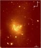 |
Fig. 23 VST g-band image (100 × 117 arcsec) of the interacting system UGC 7636. |
 |
Fig. 24 Top panel: azimuthally averaged light profiles in the g band for the five ETGs of this paper scaled to their effective parameters. Bottom panel: assembly of the (g − i) color profiles for the five ETGs and for the interacting system UGC 7636 (open circles). |
The comparison with the K+09 photometry (Fig. 21) again is quite good.
5.6. UGC 7636
As a byproduct of this paper, we also analyzed the dwarf irregular UGC 7636 (VCC1249; Nilson 1973) located 5.6′ to the southeast of NGC 4472. This object has been extensively analyzed by Arrigoni Battaia et al. (2012), who studied the tidal interaction with NGC 4472 and the gas-stripping phenomena. They found an extensive series of shells and filaments, in agreement with Janowiecki et al. (2010). Lee et al. (2000) carried out spectroscopic observations of the system and discovered an HII region associated with this galaxy but not spatially coincident with it, lying in the envelope of the giant galaxy NGC 4472.
Lacking the possibility of deriving a geometrical model of this very irregular object, we computed mean profiles by azimuthally averaging the background-corrected flux in annuli with orientation, flattening, and center all identical to that of the best ellipse encircling the visible boundaries of the object (ϵ = 0.39, PA = 0 deg and center at RA = 12h30m01.0s, Dec = +07d55m46s). The result is shown in Fig. 22. The procedure is reasonably reliable because the output changes marginally by varying the input parameters within a fair range. The method is effective in providing the trend of the color with distance. Both profiles mimic the behavior of late spiral or irregular galaxies (Capaccioli 1973). The temptation to fit the data with the sum of an r1 / 4 bulge and an exponential disk is hampered by the complexity of the body of the object (Fig. 23).
Based on Fig. 7 of Arrigoni Battaia et al. (2012), we judge that our light profiles agree with those of these authors, extending twice as deep, down to μg ~ 28.7 mag/arcsec2.
We also derived the average (g − i) color profile (Fig. 22). It reddens steadily outwards with the higher slope from a> 80 arcsec. We note, however, that in the outer range the errors are quite large. Our result agrees with that of Arrigoni Battaia et al. (2012). Outside the main galaxy body, where the SB profiles steepen, the color becomes consistent with NGC 4472 (Fig. 8), indicating a continuity between the two systems, as expected in the close interaction of the dwarf irregular with the giant elliptical.
6. Scattered light
The surface brightness levels where our estimated effects of the extended PSF are larger than twenty per cent (0.2 mag) are ~29 mag/arcsec2 in g and ~28 mag/arcsec2 in i. The following is apparent from these values:
-
1.
Typically, the azimuthally averaged light profiles derived out toa surface brightnessμg ~ 28 mag/arcsec2 are little affected by scattered light for all of our angularly small galaxies. This fact may explain the remarkable agreement between our results and those of Kormendy (Kormendy et al. 2009) because this author did not mention any correction of his light profiles, which were made using a material quite different from ours.
-
2.
The dip observed in the color profiles of NGC 4434, NGC 4464, and NGC 4467 (see Fig. 24) occurs at a surface brightness level at least two magnitudes brighter than the one where scattering becomes important.
7. Discussion and conclusions
We have presented the VST Early-type Galaxy Survey (VEGAS) that is currently ongoing with VST/OmegaCAM (PI: M. Capaccioli) and aims at studying about one hundred galaxies mainly in the southern hemisphere. The survey is as deep as the Next Generation Virgo Survey, but has no environment constraints and is expected to provide a systematic coverage of the surface photometry in at least three optical bands, g,r, and i, down to 27.3, 26.8, and 26 mag arcsec-2 (S/N> 3 per arcsec2), respectively, while u band is foreseen for a subsample of the entire survey. VEGAS is also expected to provide a census of the faint satellites (globular clusters, ultra-compact dwarfs, and dwarf galaxies; see, e.g., Cantiello et al. 2015) in the surroundings of the targeted systems, characterize their extended stellar haloes, and find evidence of the intracluster or group light around the giant galaxies in denser environments as well as signatures of merging and interactions between galaxies (e.g., tidal tails and stellar streams) and between galaxies and the group or cluster medium.
We demonstrated the typical specifications of the survey in terms of depth and photometric accuracy and illustrated the performance of the telescope and camera as well as the data reduction and data analysis approach. To this end, we chose the field of the giant elliptical galaxy NGC 4472 in the southern extension of the Virgo cluster. This is a well-studied system with extensive literature photometry to compare our results with.
In particular, we presented the deep observations in two bands (g and i). The observations were collected with the VST/OmegaCAM in March, April and May of 2013. The major advantage of this wide-field dataset is the good seeing in both filters and the uniformity of the observing conditions (data are taken within one month), which are uncommon for service-mode observations.
The surface brightness profiles of NGC 4472 reach a depth of 27.5 mag/arcsec2 in g band and 26 mag/arcsec2 in i band, which is similar to previous deep studies (see Fig. 9). This depth allowed us to spot deviations from a simple de Vaucouleurs profile and in particular a change of slope at a ~ 14′.2 (see Fig. 8) that we have associated with a decoupled ICL component that has not been detected in previous analyses (e.g., K+09). The ICL in the Virgo Cluster has been discussed before and is mainly concentrated in the cluster core. It has been detected either through direct deep imaging (Mihos et al. 2005) or using planetary nebulae as stellar light tracers (ICPNe, e.g., Arnaboldi et al. 2002; Aguerri et al. 2005). In the area around NGC 4472, evidence of ICL has been obtained with PNe by Feldmeier et al. (2004) (see also Castro-Rodriguéz et al. 2009 for a summary of ICPNe observations over a range of Virgo cluster-centric distances). However, none of these studies has addressed a detailed 2D distribution of the ICL around NGC 4472 and its connection with the giant galaxy. Here we stress that the simple inspection of the deep SB profile of NGC 4472 clearly shows a diffuse component starting to dominate at μg ~ 26.5 mag/arcsec2 (see Fig. 8), which is compatible with the typical SB values at which Zibetti et al. (2005) have observed a change of slope induced by the ICL in a series of stacked galaxy clusters.
We note that the trend of the residuals of the luminosity profiles of NGC 4472 with respect to an r1 / 4 best-fitting model has some striking analogies with the similar curve for NGC 3379 (de Vaucouleurs & Capaccioli 1979). In addition to a bright extended core, we found evidence for a wavy pattern that is possibly associated with shells of diffuse material.
We also studied the fainter ETGs in the one square degree of the OmegaCAM field: NGC 4434, NGC 4464, NGC 4467, and VCC 1199, including the dwarf irregular UGC 7636 in the proximity of the giant galaxy NGC 4472. For the two galaxies projected onto the bright halo of NGC 4472, NGC 4467 and VCC 1199, located at r ~ 4.1′ and r ~ 4.5′ from NGC 4472, we were able to estimate and subtract the galaxy background and trace the SB distribution down to μg ~ 29 mag/arcsec2 and μi ~ 27.5 mag/arcsec2, which is well beyond the nominal specifications of the survey. We reached an even greater depth for the farther systems NGC 4464 and NGC 4434, which are not (deeply) affected by the extended halo of NGC 4472 and for which we have gone down to 29−30 mag/arcsec2 in g band and ~28 mag/arcsec2 in i band. Together with the extremely good comparison with the V-band photometry by Kormendy et al. (2009), at least for our g band, this demonstrates that for normal galaxies the survey VEGAS provides an unprecedented view of the faint features around early-type galaxies, with less than one night of telescope time per galaxy (in g,r,i).
For all these systems we have highlighted some substructures that were defined as deviations from a simple de Vaucouleurs (1948) best-fit profile, as done for NGC 4472. In particular, we found evidence of bumps seen in both bands for the intermediate-luminosity systems NGC 4434 and NGC 4464. These bumps are associated with strongly varying values of the ellipticity and PA and a4 and b4 parameters, hence suggesting some substructures. They are possibly also seen in their kinematics, as for NGC 4464 (Halliday et al. 2001), but are not clearly seen in NGC 4434 (e.g., Simien & Prugniel 1997).
The color profiles, at variance with simulations (Tortora et al. 2013), do not show either the sharp decrease of the average value in the first re for objects fainter than Mg ~ − 19 or the pattern of the gradient as a function of the host galaxy absolute magnitude, which remains very flat with Mtot. We instead found an indication, which needs to be confirmed, that for r> 3re a very negative colour gradient develops in some galaxies, which apparently vanishes at r ≃ 8re (see Fig. 24).
To conclude, we illustrated the performance and accuracy achieved with the VST/OmegaCAM to produce surface photometry of early-type galaxies also in very extreme conditions. For the case of NGC 4472 the extended halo around the giant galaxy, reaching the edge of the one-square-degree field of view, has allowed us to fully test the procedure for data reduction and background subtraction. The results obtained with our observations are similar in accuracy to the collection of observations from different telescopes (see K+09). In the future we expect to implement a more general surface analysis including a wider set of photometric laws (Sersic, cored Sersics, double de Vaucouleurs, etc.) to characterize the SB measurements in a larger sample of galaxies and thus discuss results in the context of galaxy formation theories. Moreover, a forthcoming paper based on the same data as were used in the present work will be devoted to the study of small stellar systems (e.g., GCs and UCDs).
Online material
Appendix A: Data reduction
Appendix A.1: Overscan correction and master bias
For each exposure, the median value of an overscan region is computed and then subtracted, row by row. Then a masterbias, created as a sigma-clipped (5σ) average of (at least) ten bias frames, is subtracted from all the other scientific and technical exposures for full 2D bias removal.
Appendix A.2: Flat-fielding
The conversion from photons to ADUs, called gain, varies over the whole camera frame, owing to the optical design, pixel response, and electronics behavior. In principle, an exposure of a uniformly illuminated field is sufficient to build a gain-variation map. We use exposures of the sky at twilight. Because of the wide field of the instrument, these twilight flat fields may suffer from illumination variations amounting to some percent units on a degree scale. This undesired effect is mitigated by the illumination-correction procedure described below (Sect. A.5).
A master flat-field is created by averaging a set of twilight flat-fields (typically five); a sigma-clipping rejection procedure helps removing non-stationary features. The method tracks the gain variations at high spatial frequencies well, but sometimes fails at low frequencies. The reason may be the color and flux mismatch between twilight and science exposures. In this case, the twilight flat-fields are combined with some science images taken during the same night with exposure times similar to those of the images under correction. This type of frame combination has been used to process the NGC 4472 exposures. Specifically, we applied the formula  (A.1)where
 (A.2)The superscript indicates the ith CCD, the subscript low is for the low-frequency spatial component obtained by applying a low-pass spatial filter in the Fourier space. The master twilight (TFlat) and master skyflat (SFlat) are produced using a sigma-clipped average of overscan- and bias-corrected twilight frames and sky frames, respectively. The choice of the exposures used to produce the master skyflat requires special care. The dithering pattern of the exposures must be wider than the largest structure in the images (such as galaxies or the halo of bright stars) to avoid fictitious gain variations. Moreover, all the bright features in the science images (galaxies stars, halos, etc.) are accurately masked. In all these formulas, chevron brackets indicate medians done on a 1000 × 2000 pixel central spot in the CCDs.
The terms Gaini × ICi accounts for the average CCD gain and for the illumination correction and is described in Sect. A.5.
 |
Fig. A.1 Differences of magnitude among observed and SDSS DR8 equatorial stars as a function of x and y pixel coordinates. |
 |
Fig. A.2 Differences of magnitude among observed and SDSS DR8 equatorial stars as a function of x and y pixel coordinates after applying the surface fit (top). Bottom right panel: contour plot of the IC image. Bottom left panel: IC 3D view. |
Appendix A.3: Defringing
The i-band images need a correction for the fringe pattern caused by thin-film interference of sky emission lines in the detector. This is an additive component and, as such, it must be subtracted. The first step of the defringing is determining the fringing pattern by the formula  (A.3)where imsurfit indicates a fifth-order surface Chebyshev polynomial fit.
Once the pattern is found, it must be subtracted from the science image,  (A.4)using a scale factor, frscale, that is derived as follows. We assume that the fringe-pattern features are quite stable in time. We have then a priori determined the regions in the OmegaCAM frame where they clearly stand out. The best scale factor minimizes within these regions the absolute differences between peak and valley values in the fringe-corrected image.
Appendix A.4: Gain harmonization
The gain harmonization procedure sets the photometric zero point over the whole OmegaCAM mosaic. We derive the relative gain coefficients that minimize the background differences in adjacent CCDs. First we select a set of auxiliary scientific images belonging to the same night and having approximately the same exposure time as the science image to be calibrated.
Each such image is heavily clipped around the median pixel level to flag out all the sources; holes created by the procedure are filled up in a subsequent step. After overscan and bias correction, the auxiliary images are properly scaled and sigma-clipped combined. The scaling factor is calculated as the median over the scientific image divided by the median of the medians. All the holes surviving the stacking procedure are filled by interpolated values. The resulting image, corrected for the master twilight flat-frame, is then fitted with a third-order polynomial surface. This is used to compute 32 median values over subregions of 1000 × 2000 pixels centered on each CCD. These values, normalized to the median of all the CCDs medians, are the relative gain corrections. The gain harmonization correction typically ranges from 0.9 to 1.17.
Appendix A.5: Illumination correction
Another effect to be considered is the scattered light in the telescope and in the camera that is due to insufficient baffling, which produces an uncontrolled redistribution of light. In the presence of this additive contribution to the signal, the flat field is no longer an accurate model of the spatial detector response. Indeed, after flat-fielding, the image background appears perfectly flat, but the photometric response is position dependent (Andersen et al. 1995). This bias in the flat field can be mitigated by applying the illumination correction (IC) map. We determine such a map by comparing our magnitude measurements of stars observed in equatorial fields with the corresponding SDSS DR8 psf magnitudes.
The differences of magnitudes, Δm(x,y), as a function of the position are fitted with a generalized additive model (GAM; Wood 2011) to derive a surface used to correct the science images during the pre-reduction stage. GAM also provides a well-behaved surface when the standard stars do not sample the field of view uniformly, and in general the resulting image has a smoother behavior at the frame edges than do simple polynomial fits. Figures A.1 and A.2 illustrate the position dependency of the zero point before and after the IC application and the IC shape. The statistics on the differences in magnitude between the reference photometric catalog and the magnitude of sources before and after the illumination correction are the following: STD = 0.09 and MAD = 0.084 before and STD 0.05 and MAD 0.026 after the correction. The IC was created using 2189 sources. As shown in Eq. (A.1), the IC is embedded in the master flat field. In this way, the images have a uniform zero point all over the field, but the background does not appear flat. To have a flat background, the properly rescaled IC surface is also subtracted from the images.
Appendix A.6: Photometric and astrometric calibration
In VST-tube, the absolute photometric calibration is performed by observing standard star fields each night and comparing their OmegaCAM magnitudes with SDSS DR8 photometry. For the data analyzed in this work, the absolute photometric calibration was derived using 4392 sources in the g and 4489 in the i band. For each night and band, the zero point (ZP) and color term were obtained using the tool Photcal provided by Mario Radovich (Radovich et al. 2004). The extinction coefficient was derived from the extinction curve M.OMEGACAM.2011-12-01T16:15:04.474 provided by ESO. Table A.1 lists the fitted values for the zero points and color terms obtained for the nights used for the absolute photometric calibration.
Relative photometric correction among the exposures was obtained by minimizing the quadratic sum of magnitude differences between overlapping detections. The tool used for this task was SCAMP (Bertin 2006). The final coadded images were then normalized to an exposure time of one second of time and a ZP of 30 mag.
The absolute and relative astrometric calibrations were performed using SCAMP. For the absolute astrometric calibration we refer to the 2MASS catalog. Compared to this catalog, the rms of the residuals after the astrometric correction has been applied is 0.28′′. The rms on the residuals of the differences between coordinates of overlapping detections, that is, the internal astrometric accuracy, is 0.09′′. The image resampling for the application of the astrometric solution and final image coaddition is made with the program SWARP (Bertin et al. 2002).
Absolute photometric calibration for NGC 4472.
Appendix B: Convolution by the scattering profile of the point spread function
To evaluate the contribution of the scattered light, which is indeed a reason of concern for the surface photometry of galaxy outskirts, we first derived an extended stellar point spread function (PSF) by combining the unsaturated azimuthally averaged light profiles of stars of different luminosities, properly shifted in magnitudes. Our interest is not in the seeing profile, that is, in the inner few arcseconds of the PSF, but instead in the wings produced by the scattering in the mirror and in the atmosphere (Capaccioli & de Vaucouleurs 1983).
The measured PSF profiles for the g and i band are shown in Fig. B.1, normalized to unity up to the last observed point. Although the inner PSF has an average behavior that is uncorrelated with the actual seeing of each of the images contributing to the final mosaic, it could not be used for deconvolving the inner regions of the galaxy. Nonetheless, it must be kept just for providing a way to normalize the PSF itself.
To extend the PSF beyond the observational limits, we adopted the polynomial expansion of Capaccioli & de Vaucouleurs (1983), which was used to interpolate the total PSF profile (see Fig. B.1):  (B.1)where c0 = 2.187 × 10⁻⁶ (mag/arcsec2), c1 = 1.725 × 10⁻⁵, c2 = −8.559 × 10⁻⁶ and c3 = 1.570 × 10⁻⁶ for the g band and c0 = −9.497 × 10⁻⁴ (mag/arcsec2), c1 = 2.109 × 10⁻³, c2 = 1.157 × 10⁻³ and c3 = 2.134 × 10⁻⁴ for the i band. As expected, the g PSF spans a wider range than in the i band. The total integrated energy included in the inner regions, r1 / 4 ≤ 2.3, is 94% of the total flux from the stars for the g band.
 |
Fig. B.1 Adopted extended PSF for VST. |
The expressions B.1 were used to estimate the effect of the scattered light in the outskirts of the galaxies of this study, which have quite different sizes. It is indeed expected that the effect will be quite different at the same surface brightness level between angularly large and small galaxies.
Two methods were employed. The first method is a plain numerical convolution of each galaxy modeled through azimuthally averaged light profiles under the assumptions that the isophotes are ellipses of average flattening and no twisting. At first order, the difference between the model and its convolution provides an estimate of the excess of light in the observed galaxy caused by the broad smearing of the extended PSF.
Another method consists of a straightforward deconvolution of the noiseless model of the galaxy by the extended PSF. To this end, we used the IRAF task LUCY. The two methods provide very consistent results that will be illustrated in a forthcoming paper (Spavone et al., in prep.).
One additional comment is in order about the effect of the background interpolation on the partial removal of the excess of light that is due to PSF scattering. It is expected and verified numerically that small galaxies will be widely broadened by the PSF wings. If this causes the outer light profile to become much flatter, one may expect that the background interpolation procedure is capable of removing part of it, if not all. This is precisely what our numerical experiments show (Spavone et al., in prep.).
Appendix C: Additional tables
The VEGAS sample.
Surface photometry of NGC 4472.
Surface photometry of NGC 4434.
Surface photometry of NGC 4464.
Surface photometry of NGC 4467.
Surface photometry of VCC 1199.
Surface photometry of UGC 7636.
The updated status of VEGAS observations is posted at the link http://www.m2teamsoftware.it/vst/index.php/science/gto-surveys/vegas
ExAM is a code developed by Z. Huang during his Ph.D. A detailed description of the code can be found in his Ph.D. Thesis, available at the following link: http://www.fedoa.unina.it/id/eprint/8368
The reduced size with respect to the nominal VST FOV of one square degree results from a trimming of the low-weight pixels at the rim of the mosaic.
We used MINUIT (James & Roos 1975), which is a program written by staff of CERN (European Organization for Nuclear Research). It searches for minima in a user-defined function with respect to one or more parameters using several different methods as specified by the user.
IRAF (Image Reduction and Analysis Facility) is distributed by the National Optical Astronomy Observatories, which is operated by the Associated Universities for Research in Astronomy, Inc. under cooperative agreement with the National Science Foundation.
We adopted a star formation history with an exponentially decreasing rate, as is typically used for ETGs in the local Universe, with a Salpeter IMF in a metallicity range between Z⊙ and 2.5 Z⊙.
Acknowledgments
The optical imaging is collected at the ESO VLT Survey Telescope on Cerro Paranal under program ID 090.B-0414(D) and 091.B-0614(A), using the Italian INAF Guaranteed Time Observations. The data reduction for this work was carried out with the computational infrastructures of the INAF-VST Center at Naples (VSTceN). The authors wish to thank L. Ferrarese, C. Mihos, and S. Janowiecki for the data provided, C. Tortora for illuminating discussion on colors, and R. Peletier for the ongoing discussion on the best way to remove the sky background. This research made use of the NASA/IPAC Extragalactic Database (NED), which is operated by the Jet Propulsion Laboratory, California Institute of Technology, under contract with the National Aeronautics and Space Administration, and has been partly supported by the PRIN-INAF “Galaxy evolution with the VLT Survey Telescope (VST)” (PI A. Grado). M. Cantiello acknowledges support from Progetto FSE Abruzzo “Sapere e Crescita”.
References
- Aguerri, J. A. L., Gerhard, O. E., Arnaboldi, M., et al. 2005, AJ, 129, 2585 [NASA ADS] [CrossRef] [Google Scholar]
- Andersen, M. I., Freyhammer, L., & Storm, J. 1995, Calibrating and Understanding HST and ESO Instruments, ESO Conf. Proc., 53, 87 [Google Scholar]
- Arnaboldi, M., Aguerri, J. A. L., Napolitano, N. R., et al. 2002, AJ, 123, 760 [NASA ADS] [CrossRef] [Google Scholar]
- Arnaboldi, M., Ventimiglia, G., Iodice, E., Gerhard, O., & Coccato, L. 2012, A&A, 545, A37 [NASA ADS] [CrossRef] [EDP Sciences] [Google Scholar]
- Arnold, J. A., Romanowsky, A. J., Brodie, J. P., et al. 2011, ApJ, 736, L26 [NASA ADS] [CrossRef] [Google Scholar]
- Arrigoni Battaia, F., Gavazzi, G., Fumagalli, M., et al. 2012, A&A, 543, A112 [NASA ADS] [CrossRef] [EDP Sciences] [Google Scholar]
- Ashman, K. M., & Zepf, S. E. 1992, ApJ, 384, 50 [NASA ADS] [CrossRef] [Google Scholar]
- Balcells, M., Graham, A. W., & Peletier, R. F. 2007, ApJ, 665, 1104 [NASA ADS] [CrossRef] [Google Scholar]
- Bender, R., Surma, P., Doebereiner, S., Moellenhoff, C., & Madejsky, R. 1989, A&A, 217, 35 [NASA ADS] [Google Scholar]
- Bertin, E. 2006, Astronomical Data Analysis Software and Systems XV, 351, 112 [NASA ADS] [Google Scholar]
- Bertin, E., & Arnouts, S. 1996, A&AS, 117, 393 [NASA ADS] [CrossRef] [EDP Sciences] [Google Scholar]
- Bertin, E., Mellier, Y., Radovich, M., et al. 2002, Astronomical Data Analysis Software and Systems XI, 281, 228 [NASA ADS] [Google Scholar]
- Binney, J., & Petrou, M. 1985, MNRAS, 214, 449 [NASA ADS] [CrossRef] [Google Scholar]
- Blom, C., Forbes, D. A., Brodie, J. P., et al. 2012, MNRAS, 426, 1959 [NASA ADS] [CrossRef] [Google Scholar]
- Brodie, J. P., Usher, C., Conroy, C., et al. 2012, ApJ, 759, L33 [NASA ADS] [CrossRef] [Google Scholar]
- Brodie, J. P., Romanowsky, A. J., Strader, J., et al. 2014, ApJ, 796, 52 [NASA ADS] [CrossRef] [Google Scholar]
- Bruzual, G., & Charlot, S. 2003, MNRAS, 344, 1000 [NASA ADS] [CrossRef] [Google Scholar]
- Cantiello, M., Grado, A., Blakeslee, J. P., et al. 2013, A&A, 552, A106 [NASA ADS] [CrossRef] [EDP Sciences] [Google Scholar]
- Cantiello, M., Capaccioli, M., Napolitano, N., et al. 2015, A&A, 576, A14 [NASA ADS] [CrossRef] [EDP Sciences] [Google Scholar]
- Caon, N., Capaccioli, M., & D’Onofrio, M. 1993, MNRAS, 265, 1013 [NASA ADS] [CrossRef] [Google Scholar]
- Caon, N., Capaccioli, M., & D’Onofrio, M. 1994, A&AS, 106, 199 [NASA ADS] [Google Scholar]
- Capaccioli, M. 1973, Mem. Soc. Astron. Italiana, 44, 417 [NASA ADS] [Google Scholar]
- Capaccioli, M. 1988, Bol. Acad. Nac. Cienc. Cordoba, Argent., Tomo, 58, 317 [Google Scholar]
- Capaccioli, M., & de Vaucouleurs, G. 1983, ApJS, 52, 465 [NASA ADS] [CrossRef] [Google Scholar]
- Capaccioli, M., & Schipani, P. 2011, The Messenger, 146, 2 [NASA ADS] [Google Scholar]
- Capaccioli, M., Caon, N., & D’Onofrio, M. 1992, MNRAS, 259, 323 [NASA ADS] [CrossRef] [Google Scholar]
- Carlberg, R. G. 1984, ApJ, 286, 403 [NASA ADS] [CrossRef] [Google Scholar]
- Castro-Rodriguéz, N., Arnaboldi, M., Aguerri, J. A. L., et al. 2009, A&A, 507, 621 [NASA ADS] [CrossRef] [EDP Sciences] [Google Scholar]
- Chen, C.-W., Côté, P., West, A. A., Peng, E. W., & Ferrarese, L. 2010, ApJS, 191, 1 [NASA ADS] [CrossRef] [Google Scholar]
- Coccato, L., Gerhard, O., Arnaboldi, M., et al. 2009, MNRAS, 394, 1249 [NASA ADS] [CrossRef] [Google Scholar]
- Coccato, L., Gerhard, O., & Arnaboldi, M. 2010, MNRAS, 407, L26 [NASA ADS] [Google Scholar]
- Côté, P., Marzke, R. O., & West, M. J. 1998, ApJ, 501, 554 [NASA ADS] [CrossRef] [Google Scholar]
- Côté, P., Blakeslee, J. P., Ferrarese, L., et al. 2004, ApJS, 153, 223 [NASA ADS] [CrossRef] [Google Scholar]
- Côté, P., Ferrarese, L., Jordán, A., et al. 2007, ApJ, 671, 1456 [NASA ADS] [CrossRef] [Google Scholar]
- D’Abrusco, R., Fabbiano, G., & Zezas, A. 2015, ApJ, 805, 26 [NASA ADS] [CrossRef] [Google Scholar]
- Daddi, E., Renzini, A., Pirzkal, N., et al. 2005, ApJ, 626, 680 [NASA ADS] [CrossRef] [Google Scholar]
- de Jong, J. T. A., Verdoes Kleijn, G. A., Kuijken, K. H., & Valentijn, E. A. 2013, Exp. Astron., 35, 25 [Google Scholar]
- de Vaucouleurs, G. 1948, Ann. Astrophys., 11, 247 [Google Scholar]
- de Vaucouleurs, G., & Capaccioli, M. 1979, ApJS, 40, 699 [NASA ADS] [CrossRef] [Google Scholar]
- de Vaucouleurs, G., de Vaucouleurs, A., Corwin, H. G., Jr., et al. 1991, Third Reference Catalogue of Bright Galaxies, Vol. I: Explanations and references, Vol. II: Data for galaxies between 0h and 12h, Vol. III: Data for galaxies between 12h and 24h (New York: Springer) [Google Scholar]
- Duc, P.-A., Cuillandre, J.-C., Karabal, E., et al. 2015, MNRAS, 446, 120 [NASA ADS] [CrossRef] [Google Scholar]
- Feldmeier, J. J., Ciardullo, R., Jacoby, G. H., & Durrell, P. R. 2004, ApJ, 615, 196 [NASA ADS] [CrossRef] [Google Scholar]
- Ferrarese, L., Côté, P., Jordán, A., et al. 2006, ApJS, 164, 334 [NASA ADS] [CrossRef] [Google Scholar]
- Ferrarese, L., Côté, P., Cuillandre, J.-C., et al. 2012, ApJS, 200, 4 [NASA ADS] [CrossRef] [Google Scholar]
- Forbes, D. A., Brodie, J. P., & Grillmair, C. J. 1997, AJ, 113, 1652 [NASA ADS] [CrossRef] [Google Scholar]
- Forbes, D. A., Spitler, L. R., Strader, J., et al. 2011, MNRAS, 413, 2943 [NASA ADS] [CrossRef] [Google Scholar]
- Gonzalez, A. H., Zabludoff, A. I., & Zaritsky, D. 2005, ApJ, 618, 195 [Google Scholar]
- Grado, A., Capaccioli, M., Limatola, L., & Getman, F. 2012, Mem. Soc. Astron. It. Suppl., 19, 362 [Google Scholar]
- Halliday, C., Davies, R. L., Kuntschner, H., et al. 2001, MNRAS, 326, 473 [NASA ADS] [CrossRef] [Google Scholar]
- Hopkins, P. F., Bundy, K., Hernquist, L., Wuyts, S., & Cox, T. J. 2010, MNRAS, 401, 1099 [NASA ADS] [CrossRef] [Google Scholar]
- Huang, Z., Radovich, M., Grado, A., et al. 2011, A&A, 529, A93 [NASA ADS] [CrossRef] [EDP Sciences] [Google Scholar]
- Ibata, R. A., Gilmore, G., & Irwin, M. J. 1994, Nature, 370, 194 [NASA ADS] [CrossRef] [Google Scholar]
- James, F., & Roos, M. 1975, Comput. Phys. Commun., 10, 343 [NASA ADS] [CrossRef] [PubMed] [Google Scholar]
- Janowiecki, S., Mihos, J. C., Harding, P., et al. 2010, ApJ, 715, 972 [NASA ADS] [CrossRef] [Google Scholar]
- Jedrzejewski, R. I. 1987, MNRAS, 226, 747 [Google Scholar]
- Jordán, A., Blakeslee, J. P., Côté, P., et al. 2007, ApJS, 169, 213 [NASA ADS] [CrossRef] [Google Scholar]
- Kim, E., Lee, M. G., & Geisler, D. 2000, MNRAS, 314, 307 [NASA ADS] [CrossRef] [Google Scholar]
- Kormendy, J. 1985, ApJ, 295, 73 [NASA ADS] [CrossRef] [Google Scholar]
- Kormendy, J., Fisher, D. B., Cornell, M. E., & Bender, R. 2009, ApJS, 182, 216 [NASA ADS] [CrossRef] [Google Scholar]
- Kuijken, K. 2011, The Messenger, 146, 8 [NASA ADS] [Google Scholar]
- Lee, H., Richer, M. G., & McCall, M. L. 2000, ApJ, 530, L17 [NASA ADS] [CrossRef] [Google Scholar]
- Mei, S., Blakeslee, J. P., Côté, P., et al. 2007, ApJ, 655, 144 [NASA ADS] [CrossRef] [Google Scholar]
- Mihos, J. C., Harding, P., Feldmeier, J., & Morrison, H. 2005, ApJ, 631, L41 [NASA ADS] [CrossRef] [Google Scholar]
- Mihos, J. C., Harding, P., Rudick, C. S., & Feldmeier, J. J. 2013, ApJ, 764, L20 [NASA ADS] [CrossRef] [Google Scholar]
- Napolitano, N. R., Romanowsky, A. J., Coccato, L., et al. 2009, MNRAS, 393, 329 [NASA ADS] [CrossRef] [Google Scholar]
- Napolitano, N. R., Pota, V., Romanowsky, A. J., et al. 2014, MNRAS, 439, 659 [NASA ADS] [CrossRef] [Google Scholar]
- Nilson, P. 1973, Nova Acta Regiae Soc. Sci. Upsaliensis, Ser. V [Google Scholar]
- Oser, L., Ostriker, J. P., Naab, T., Johansson, P. H., & Burkert, A. 2010, ApJ, 725, 2312 [NASA ADS] [CrossRef] [Google Scholar]
- Peletier, R. F., Davies, R. L., Illingworth, G. D., Davis, L. E., & Cawson, M. 1990, AJ, 100, 1091 [NASA ADS] [CrossRef] [Google Scholar]
- Peng, E. W., Jordán, A., Côté, P., et al. 2006, ApJ, 639, 95 [NASA ADS] [CrossRef] [Google Scholar]
- Pipino, A., D’Ercole, A., & Matteucci, F. 2008, A&A, 484, 679 [NASA ADS] [CrossRef] [EDP Sciences] [Google Scholar]
- Pohlen, M., & Trujillo, I. 2006, A&A, 454, 759 [NASA ADS] [CrossRef] [EDP Sciences] [Google Scholar]
- Proctor, R. N., Forbes, D. A., Romanowsky, A. J., et al. 2009, MNRAS, 398, 91 [NASA ADS] [CrossRef] [Google Scholar]
- Prugniel, P., & Simien, F. 1996, A&A, 309, 749 [NASA ADS] [Google Scholar]
- Simien, F., & Prugniel, P. 1997, A&AS, 122, 521 [NASA ADS] [CrossRef] [EDP Sciences] [Google Scholar]
- Radovich, M., Arnaboldi, M., Ripepi, V., et al. 2004, A&A, 417, 51 [NASA ADS] [CrossRef] [EDP Sciences] [Google Scholar]
- Romanowsky, A. J., Douglas, N. G., Arnaboldi, M., et al. 2003, Science, 301, 1696 [NASA ADS] [CrossRef] [PubMed] [Google Scholar]
- Romanowsky, A. J., Strader, J., Spitler, L. R., et al. 2009, AJ, 137, 4956 [NASA ADS] [CrossRef] [Google Scholar]
- Romanowsky, A. J., Strader, J., Brodie, J. P., et al. 2012, ApJ, 748, 29 [NASA ADS] [CrossRef] [Google Scholar]
- Saglia, R. P., Maraston, C., Thomas, D., Bender, R., & Colless, M. 2002, ApJ, 579, L13 [NASA ADS] [CrossRef] [Google Scholar]
- Shen, S., Mo, H. J., White, S. D. M., et al. 2003, MNRAS, 343, 978 [NASA ADS] [CrossRef] [Google Scholar]
- Tal, T., van Dokkum, P. G., Nelan, J., & Bezanson, R. 2009, AJ, 138, 1417 [NASA ADS] [CrossRef] [Google Scholar]
- Tonry, J., & Schneider, D. P. 1988, AJ, 96, 807 [NASA ADS] [CrossRef] [Google Scholar]
- Tortora, C., Romeo, A. D., Napolitano, N. R., et al. 2011, MNRAS, 411, 627 [NASA ADS] [CrossRef] [Google Scholar]
- Tortora, C., Pipino, A., D’Ercole, A., Napolitano, N. R., & Matteucci, F. 2013, MNRAS, 435, 786 [NASA ADS] [CrossRef] [Google Scholar]
- Usher, C., Forbes, D. A., Brodie, J. P., et al. 2012, MNRAS, 426, 1475 [NASA ADS] [CrossRef] [Google Scholar]
- Usher, C., Forbes, D. A., Brodie, J. P., et al. 2015, MNRAS, 446, 369 [NASA ADS] [CrossRef] [Google Scholar]
- van Dokkum, P. G., Whitaker, K. E., Brammer, G., et al. 2010, ApJ, 709, 1018 [NASA ADS] [CrossRef] [Google Scholar]
- Watkins, A. E., Mihos, J. C., Harding, P., & Feldmeier, J. J. 2014, ApJ, 791, 38 [NASA ADS] [CrossRef] [Google Scholar]
- Whitmore, B. C., & Bell, M. 1988, ApJ, 324, 741 [NASA ADS] [CrossRef] [Google Scholar]
- Wood, S.N. 2011, J. Roy. Stat. Soc. (B), 73, 3 [Google Scholar]
- Yoon, S.-J., Yi, S. K., & Lee, Y.-W. 2006, Science, 311, 1129 [NASA ADS] [CrossRef] [PubMed] [Google Scholar]
- Zibetti, S., White, S. D. M., & Brinkmann, J. 2004, MNRAS, 347, 556 [NASA ADS] [CrossRef] [Google Scholar]
- Zibetti, S., White, S. D. M., Schneider, D. P., & Brinkmann, J. 2005, MNRAS, 358, 949 [Google Scholar]
All Tables
Effective parameters of the r1 / 4 models that best fit our light profiles outside the seeing-blurred cores.
Average colors computed as shifts giving the best match of the inner light profiles.
All Figures
|
Fig. 1 VEGAS potential target distribution in the parameter space (blue points). Higher priority is given to galaxies with HST data (red circles) and Chandra/XMM data (yellow dots). We note that close systems are observed in a single VST/OmegaCAM pointing in many cases. |
| In the text | |
|
Fig. 2 VST color composite image of the 0.9° × 0.8° field around the giant galaxy NGC 4472 from g and i band VEGAS images. Circles mark the other four ETGs studied in this paper and the interacting system UGC 7636. |
| In the text | |
|
Fig. 3 VST g-band mosaic of NGC 4472 showing the masking of bright sources in the field, done either automatically or manually depending on the brightness of the sources. |
| In the text | |
|
Fig. 4 VST g-band mosaic of NGC 4472. The isophotal contour (in white) represents the last isophote fitted to obtain the surface brightness profile. The image size is 0.9° × 0.8°. |
| In the text | |
|
Fig. 5 Azimuthally averaged intensity profile of NGC 4472 as a function of the semi-major axis. The horizontal line indicates the residual background counts of Δsky ~ 0.3. |
| In the text | |
|
Fig. 6 Left: false-color image of the VST pointing of NGC 4472, trimmed to the same size as that in Fig. 4. The magnitude scale adopted to produce the picture is shown at the bottom. The last clearly visible isophote is at μg ~ 27 mag/arcsec2. Right: residual image obtained by subtracting from the left picture the galaxy model described in Sect. 5.1.2. Masks adopted to exclude features from the fitting are shown as circles. |
| In the text | |
|
Fig. 7 NGC 4472. Top: position angle (PA) and ellipticity (ϵ) profiles in the g and i bands compared with those in K+09. Bottom: isophotal shape parameters in the g and i bands. |
| In the text | |
|
Fig. 8 NGC 4472. Top: azimuthally averaged light profiles in the g (blue) and i (red) bands. Bottom: (g − i) color profile in the region (a> 2 arcsec) unaffected by differential seeing. The red dots trace the (B − V) profile published by Mihos et al. (2013) shifted by +0.25 mag, measured in the regions of high S/N for both datasets. The comparison supports the blueward gradient that we found for a/ae> 4, although with very large errors. |
| In the text | |
|
Fig. 9 NGC 4472. Top panel: azimuthally averaged g-band profile from VEGAS compared to literature. The color code of the symbols mimicks the corresponding photometric bands. Arbitrary shifts have been used to match with the VEGAS profile. In particular, the B-band profile byMihos et al. (2013) has been shifted by −0.35 mag, the V band from Kormendy et al. (2009) and Janowiecki et al. (2010) by +0.35 mag, and the profile by Kim et al. (2000) by +0.92 mag. Bottom panel: (O–C) residuals of mean profiles from a best-fitting r1 / 4 model used only to remove the main gradient and facilitate comparison. The blue solid line plots the (O–C) residuals for the east-west photometric cross-section of the standard elliptical galaxy NGC 3379 from de Vaucouleurs & Capaccioli (1979). There are clear similarities: the bright core and a wavy trend overimposed on the smooth r1 / 4 trend. |
| In the text | |
|
Fig. 10 NGC 4472. Unsharp masked image, extracted from the whole VST mosaic (500 × 600 arcsec) in the i (left panel) and g band (right panel). Lighter colors correspond to brighter features. |
| In the text | |
|
Fig. 11 NGC 4472. Left panel: a region of 55 × 56 arcmin of the VST g band mosaic. Right panel: 2D model (see text). |
| In the text | |
|
Fig. 12 NGC 4472. Zoom (37 × 35 arcmin) of the median-smoothed residual image. The outermost elliptical contour marks the region where the b-model subtraction was not applied. The superimposed white contours are 1) the tail connecting UGC 7636 to the giant ETG; and 2) shells and fan of material identified by Janowiecki et al. (2010) and Arrigoni Battaia et al. (2012) that is visible in our residual image. The wave-like residuals, concentric with the NGC 4472 nucleus, are spuriously introduced by the numerical procedure. |
| In the text | |
|
Fig. 13 Long tail connecting UGC 7636 with the core of NGC 4472, from a double-folding subtraction. The image size is 15 × 15 arcmin. |
| In the text | |
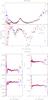 |
Fig. 14 Same as Fig. 7 for NGC 4434. |
| In the text | |
|
Fig. 15 NGC 4434. Top panel: azimuthally averaged light profiles in the g (blue) and i (red) bands. Center panel: (O−C) residuals of the VEGAS profiles and the V-band profile of K+09 with respect to the best-fitting r1 / 4 model (see Table 4). The best match is obtained with the shifts listed in Table 5. VEGAS data for a1 / 4< 1.2 are affected by seeing. Bottom panel: (g − i) color profile. Again the data at a1 / 4< 1.2 have not been corrected for seeing. |
| In the text | |
 |
Fig. 16 Same as Fig. 7 for NGC 4464. |
| In the text | |
 |
Fig. 17 Same as Fig. 15 for NGC 4464. |
| In the text | |
 |
Fig. 18 Same as Fig. 7 for NGC 4467. |
| In the text | |
 |
Fig. 19 Same as Fig. 15 for NGC 4467. |
| In the text | |
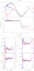 |
Fig. 20 Same as Fig. 7 for VCC 1199. |
| In the text | |
 |
Fig. 21 Same as Fig. 15 for VCC 1199. |
| In the text | |
|
Fig. 22 UGC 7636. Top panel: azimuthally averaged light profiles in the g (blue dots) and i (red dots) bands. Bottom panel: (g − i) color profile. |
| In the text | |
|
Fig. 23 VST g-band image (100 × 117 arcsec) of the interacting system UGC 7636. |
| In the text | |
|
Fig. 24 Top panel: azimuthally averaged light profiles in the g band for the five ETGs of this paper scaled to their effective parameters. Bottom panel: assembly of the (g − i) color profiles for the five ETGs and for the interacting system UGC 7636 (open circles). |
| In the text | |
|
Fig. A.1 Differences of magnitude among observed and SDSS DR8 equatorial stars as a function of x and y pixel coordinates. |
| In the text | |
|
Fig. A.2 Differences of magnitude among observed and SDSS DR8 equatorial stars as a function of x and y pixel coordinates after applying the surface fit (top). Bottom right panel: contour plot of the IC image. Bottom left panel: IC 3D view. |
| In the text | |
|
Fig. B.1 Adopted extended PSF for VST. |
| In the text | |
Current usage metrics show cumulative count of Article Views (full-text article views including HTML views, PDF and ePub downloads, according to the available data) and Abstracts Views on Vision4Press platform.
Data correspond to usage on the plateform after 2015. The current usage metrics is available 48-96 hours after online publication and is updated daily on week days.
Initial download of the metrics may take a while.