| Issue |
A&A
Volume 581, September 2015
|
|
|---|---|---|
| Article Number | A112 | |
| Number of page(s) | 13 | |
| Section | The Sun | |
| DOI | https://doi.org/10.1051/0004-6361/201526250 | |
| Published online | 16 September 2015 | |
Characterizing the propagation of gravity waves in 3D nonlinear simulations of solar-like stars
1
Laboratoire AIM Paris-Saclay, CEA/DSM −
CNRS − Université Paris Diderot, IRFU/SAp Centre de Saclay,
91191
Gif-sur-Yvette,
France
e-mail: This email address is being protected from spambots. You need JavaScript enabled to view it.
; This email address is being protected from spambots. You need JavaScript enabled to view it.
2
Département de physique, Université de Montréal,
CP 6128 Succ. Centre-Ville, QC
H3C-3J7
Montréal,
Canada
Received: 2 April 2015
Accepted: 4 June 2015
Abstract
Context. The revolution of helio- and asteroseismology provides access to the detailed properties of stellar interiors by studying the star’s oscillation modes. Among them, gravity (g) modes are formed by constructive interferences between progressive internal gravity waves (IGWs), propagating in stellar radiative zones. Our new 3D nonlinear simulations of the interior of a solar-like star allows us to study the excitation, propagation, and dissipation of these waves.
Aims. The aim of this article is to clarify our understanding of the behavior of IGWs in a 3D radiative zone and to provide a clear overview of their properties.
Methods. We use a method of frequency filtering that reveals the path of individual gravity waves of different frequencies in the radiative zone.
Results. We are able to identify the region of propagation of different waves in 2D and 3D, to compare them to the linear raytracing theory and to distinguish between propagative and standing waves (g-modes). We also show that the energy carried by waves is distributed in different planes in the sphere, depending on their azimuthal wave number.
Conclusions. We are able to isolate individual IGWs from a complex spectrum and to study their propagation in space and time. In particular, we highlight in this paper the necessity of studying the propagation of waves in 3D spherical geometry, since the distribution of their energy is not equipartitioned in the sphere.
Key words: hydrodynamics / stars: interiors / Sun: interior / turbulence / waves
© ESO, 2015
1. Introduction
Internal gravity waves (IGWs) propagate in stably stratified fluids with gravity as a restoring force. They can be observed in laboratory experiments (e.g., Mowbray & Rarity 1967; Gostiaux et al. 2007; Perrard et al. 2013), planetary atmospheres and oceans (e.g., Staquet & Sommeria 2002; Fritts & Alexander 2003), and in our case, they are believed to exist in the radiative regions of stars. In solar-like stars, these waves are stochastically excited by turbulent convective motions in the outer layers, which leads to the formation of a rich spectrum. During their propagation, IGWs are known to transport angular momentum by radiative damping (e.g., Schatzman 1993; Zahn et al. 1997), corotation resonances (e.g., Booker & Bretherton 1967; Alvan et al. 2013), or nonlinear wave breaking (e.g., Barker & Ogilvie 2010). They also affect the mixing of chemical elements in stars’ interiors (e.g., Press 1981; Garcia Lopez & Spruit 1991; Montalban 1994; Charbonnel & Talon 2005). As a consequence, they are expected to influence the evolution of stars and particularly the evolution of their internal rotation profiles (Talon & Charbonnel 2005; Charbonnel et al. 2013; Mathis et al. 2013). In the solar case, IGWs are serious candidates for explaining the solid-body rotation of its radiative interior down to 0.2 R⊙ (Kumar et al. 1999; Charbonnel & Talon 2005)1. They are also invoked to explain the transport of angular momentum in sub- and redgiant stars (Talon & Charbonnel 2008; Fuller et al. 2014) and in intermediate mass and massive stars (Pantillon et al. 2007; Lee et al. 2014).
When progressive waves interfere constructively, they form standing modes called gravity (g) modes, whose measurement can provide information about the structure of the stars’ deep interiors. These individual g-modes remain barely detectable at the surface of the Sun. Unlike acoustic (p) modes, mainly located near the surface, g-modes are trapped in the inner radiative region, so we can accumulate a lot of information about the structure of this zone. Nevertheless, they are evanescent in convective regions and thus reach the surface with small amplitudes (Appourchaux et al. 2010, and references therein). As of today, the only reported detection for the Sun has been done in Garcia et al. (2007, 2008). They observed the asymptotic signature of g-modes at the surface of the Sun, but we are not yet able to detect individual peaks (Garcia 2009). To improve our ability to detect them, we thus need to characterize their properties, time variabilities, and ability to tunnel through the solar convection zone better.
Realistic numerical simulations help for understanding the properties of IGWs in stars. Their excitation by the pummeling of convective plumes at the top of the radiative zone has already been studied in 2D (Massaguer et al. 1984; Hurlburt et al. 1986, 1994; Kiraga et al. 2003; Dintrans et al. 2005; Rogers & Glatzmaier 2005; Rogers et al. 2006) and in 3D (Saikia et al. 2000; Brummell et al. 2002; Browning et al. 2004; Kiraga et al. 2005; Brun et al. 2011). Recently, Alvan et al. (2014) have shown the substantial progress made in high-performance computing, allowing a 3D solar-like star to be modeled in full spherical geometry from r = 0 to r = 0.97 R⊙. They took the nonlinear coupling between the convective envelope, the radiative interior, and the dissipation along the wave propagation into account. Thanks to the use of a realistic density stratification in the radiative region, the properties and frequencies of the waves excited by the convection are those expected from theory. We seek here to characterize the spectrum excited better by doing a detailed analysis of its substructures. More precisely, we want to understand why we can see modes in the spectral space and not in the direct observation of the simulation (real space). Our guiding question concerns the distinction between progressive and standing waves and the transition between these two families. Finally, we see how the waves’ energy is distributed in the spherical star and what can be deduced from their excitation.
In the present work, we use a method of frequency filtering that reveals the signature of IGWs in real space and that clarifies their behavior at different frequencies. In Sect. 2, we show and discuss the complex and rich spectrum of IGWs excited by penetrative convection in our 3D model. In Sect. 3, we describe our method of frequency filtering before presenting the associated results. We thus show the relation between our full 3D nonlinear simulations and the asymptotic linear raytracing theory, often used to illustrate the propagation of internal waves in stars. We also show that waves of low frequency are attenuated while higher-frequency waves propagate up to the center and form modes. We finish by showing a property of internal waves that single-handedly warrants their study in 3D: at low rotation rate, the energy carried by IGWs is concentrated in planes of the sphere, whose inclination depends on the wave numbers. This property is broken at high rotation rates, leading to very complex 3D waves’ paths of propagation.
2. 3D nonlinear simulations of IGWs
We used the anelastic spherical harmonic (ASH) code (Clune et al. 1999; Brun et al. 2004) to solve the full set of 3D anelastic hydrodynamic equations in a solar-like star rotating at the velocity Ω0 = Ω0ez (Ω0 = 414 nHz). The domain of computation includes both the radiative and the convective regions from r = 0 up to r = 0.97 R⊙. We provide a description of the ASH code and a presentation of the model used here in Appendix A. More details can be found in Alvan et al. (2014). In this section, we focus on the study of the gravity wave spectrum excited in the radiative zone. This spectrum is rich and complex, and it varies as a function of depth.
2.1. Wave pattern in physical space
The use of a seismically calibrated 1D solar model (Brun
et al. 2002) to initialize the 3D simulation ensures a realistic stratification
in the radiative zone that allows us to study the properties of the IGWs excited by the
overshoot process quantitatively. To quantify this stratification, we define the
Brunt-Väisälä frequency by 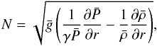 (1)where
r is the
radius,
(1)where
r is the
radius,  ,
,
 ,
and
,
and  are the reference density, pressure, and acceleration of gravity, and γ is the first adiabatic
exponent (see Appendix A). In the whole paper, frequencies are plotted in Hz and not in
rad/s. We represent the profile of N in Fig. 1.
are the reference density, pressure, and acceleration of gravity, and γ is the first adiabatic
exponent (see Appendix A). In the whole paper, frequencies are plotted in Hz and not in
rad/s. We represent the profile of N in Fig. 1.
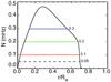 |
Fig. 1 Profile of the Brunt-Väisälä frequency as a function of the normalized radius. Colored horizontal lines highlight the regions of propagation of the waves revealed by our filtering technique in Fig. 5. |
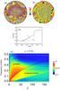 |
Fig. 2 a) 3D rendering of the simulated star. We represent the radial velocity divided by its rms value at each radius. b) Equatorial slice. Like in the 3D view, IGWs pattern are visible in the inner radiative zone as quasi-circular spirals. c) rms profiles of the total (solid line) and radial (dotted line) velocities as a function of the normalized radius, averaged over longitude, latitude, and time (about 10 convective overturning times). d) Energy spectrum of gravity waves computed at r0 = 0.5 R⊙ as a function of degree ℓ and frequency ω. Ridges are formed by g-modes of same radial order n, and we see that they tend to the maximum Brunt-Väisälä frequency at high order ℓ (dotted white line). The black solid line denotes the separation between g-modes (above) and progressive waves (below). |
The linear asymptotic theory (e.g., Unno et al.
1989; Aerts et al. 2010; Christensen-Dalsgaard 2011) predicts that the
dispersion relation of IGWs is  (2)where
ω is the
frequency of the wave (also expressed in Hz), and k the norm of the
wavevector k =
krer +
kh whose radial and
horizontal components are denoted kr and kh. This
equation is satisfied when we neglect the effect of the Coriolis acceleration, which is
possible here since the model rotates at the solar rotation rate, verifying
2Ω0 = 2 × 414 nHz
≪ ω for the
frequencies ω
of interest in this work. According to this relation, IGWs can propagate in the regions
where N is
real only, i.e. in radiative zones, and are evanescent in convective zones. Their maximum
frequency is also limited by the maximum value max(N) = 0.466 mHz available
for the current Sun (cf. Fig. 1).
(2)where
ω is the
frequency of the wave (also expressed in Hz), and k the norm of the
wavevector k =
krer +
kh whose radial and
horizontal components are denoted kr and kh. This
equation is satisfied when we neglect the effect of the Coriolis acceleration, which is
possible here since the model rotates at the solar rotation rate, verifying
2Ω0 = 2 × 414 nHz
≪ ω for the
frequencies ω
of interest in this work. According to this relation, IGWs can propagate in the regions
where N is
real only, i.e. in radiative zones, and are evanescent in convective zones. Their maximum
frequency is also limited by the maximum value max(N) = 0.466 mHz available
for the current Sun (cf. Fig. 1).
In Figs. 2a and b, we show the radial velocity in a 3D view and an equatorial slice of the simulated star with downflows and upflows. We clearly see the convective envelope from about 0.71 R⊙ to the surface of the computational domain and the inner radiative zone. Since it is visible in Fig. 2c, the velocity amplitude of the convective motions is much larger than the one of the waves (factor 103 to 105). Consequently, to visualize both convection pattern and IGWs in the top panels, we divided the radial velocity by its root mean square (rms) value at each radius.
In the radiative region, we see what looks like concentric circles, which are in fact almost circular spirals. They correspond to the superposition of several wavefronts of gravity waves evolving at different frequencies. The comparison between these pattern and those predicted by the raytracing theory (see Sect. 3.2) shows that the IGWs visualized here have frequencies of about [0.01−0.05] mHz. This is quite low in comparison with the expected solar g-modes’ frequencies (Christensen-Dalsgaard 2011). Deeper in the radiative region, the quasi-circular pattern changes into a more complex shape. We explain these observations in Sect. 3.3.
2.2. Spectrum
To describe the IGWs we can see into the radiative zone more precisely, we represent
their spectrum so as to calculate their frequencies. It is obtained by applying a
spherical harmonic transform, followed by a temporal Fourier transform, to the radial
velocity vr(r0,θ,ϕ,t).
For the moment, the radius r0 is fixed, and we obtain the quantity
 , where ℓ is the degree,
m azimuthal
number, and ω
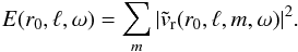
the frequency of the wave. The quantity represented in Fig. 2d is obtained by adding all contributions in m quadratically, such as
, where ℓ is the degree,
m azimuthal
number, and ω
the frequency of the wave. The quantity represented in Fig. 2d is obtained by adding all contributions in m quadratically, such as
 (3)The
length of the temporal sequence used here is about 30 days, which provides a frequency
resolution of ωmin
≈ 0.38 × 10⁻³ mHz. The temporal sampling rate
Δt = 1000 s
allows us to reach the maximum (Nyquist) frequency ωmin = 0.5 mHz
and corresponds to ten times the time step of the simulation.
(3)The
length of the temporal sequence used here is about 30 days, which provides a frequency
resolution of ωmin
≈ 0.38 × 10⁻³ mHz. The temporal sampling rate
Δt = 1000 s
allows us to reach the maximum (Nyquist) frequency ωmin = 0.5 mHz
and corresponds to ten times the time step of the simulation.
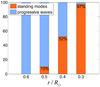 |
Fig. 3 Percentage of the total energy (squared radial velocity) distributed in standing and progressive gravity waves. |
The figure we obtained (Fig. 2d) is close to the spectrum predicted by the linear theory (e.g., Provost & Berthomieu 1986; Christensen-Dalsgaard 2003). In the higher part of the spectrum (above the black curve), we see individual modes forming energy peaks. Their frequencies correspond to g-mode frequencies calculated by the oscillation code ADIPLS2 with very good accuracy (Alvan et al. 2014). Modes with the same radial order n− corresponding to the number of zeros of the radial eigenfunctions − form ridges, particularly visible at high frequency. Moreover, as predicted by the dispersion relation (Eq. (2)), the frequency upper limit corresponds to max(N) = 0.466 mHz. The lower limit of this “g-modes” region is the effect of waves attenuation. It is shown here and can be understood as a cut-off frequency for the formation of g-modes, under which the waves are sufficiently damped so that standing modes cannot form. We show in Appendix B that this curve behaves as [ℓ(ℓ + 1)]3/8.
Below this frontier, the spectrum is composed of progressive waves. When we compare spectra at different radii r0 (Alvan et al. 2014), we see that the “progressive-wave region” decreases with increasing depth and finally disappears. We compare the proportion of energy distributed in both regions in Fig. 3. At r = 0.6 R⊙, the whole energy is contained in progressive waves. Then, when we move deeper into the radiative zone, g-modes appear and progressive waves are damped. Below 0.3 R⊙, the number of progressive waves becomes negligible, and the whole energy of the spectrum corresponds to standing modes.
The richness of this spectrum shows that a wide frequency range is excited by convection. As a result, one may wonder why we only see one main pattern in real space (Figs. 2a and b). The raytracing theory predicts that IGWs propagate along different paths depending on their frequencies. Is there a way to visualize these paths in our simulations? By isolating some waves and visualizing them in the model, we show that we can learn more about the regions of propagation of IGWs in a full 3D geometry.
3. Going further: frequency filtering of radiative zone
Here, we have filtered our data by selecting only a narrow band of frequencies. In the following sections, we show that this method reveals important properties of IGWs that were not accessible before.
3.1. Method
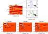 |
Fig. 4 Filtering of the same image at three different frequencies. Downflows are represented in blue, upflows in red tones. A) Selected zone of the star. B) and C) frequency spectra of points B) and C) where we see one or two main peaks. The vertical axis represents the normalized radial velocity. The vertical red line indicates the position of the Gaussian filter (width = 2 × 10⁻⁴ mHz). D1), D2) and D3): result of the filtering of image A) at three frequencies. Wave beams are visible with an inclination that varies with the frequency, forming St Andrew’s crosses. The angles’ values are indicated in Table 1. |
The idea of the frequency filtering can be discussed as follows. We illustrate the method in Fig. 4.
Panel (A) shows a region of the simulated star belonging to the equatorial plane. We represent the radial velocity as a function of the radius and the longitude, right below the excitation zone (interface between convective and radiative regions). Several different gravity waves are propagating through this region, but they are placed on top of each other so we cannot see their paths clearly. Our aim is to separate the waves of different frequencies. To illustrate the manipulation, we have chosen two points (B and C) labeled by white crosses. Image (A) evolves with time and so does the signal at points B and C.
Panels (B) and (C) represent the Fourier spectrum of these two points. For Point B, we see that the main peak is located in the blue shaded region, around 0.01−0.02 mHz. For Point C, the main peak is instead around 0.03 mHz (green shaded region) but we also see a secondary peak around 0.005 mHz (orange shaded region). This means that each point oscillates at the frequency of one or two waves passing through.
Thus, to isolate a wave oscillating at frequency 0.02 mHz (for example), we calculated the Fourier spectrum of each point (i.e. Nr × Nθ × Nϕ = 569 × 512 × 1024 ≈ 3 × 10⁸ points), we applied a passband filter to the spectrum (a Gaussian centered at 0.02 mHz), and we came back to the real space using an inverse Fourier transform. The width of the Gaussian filter is 2 × 10⁻⁴ mHz for this example.
The result is shown in Panels (D1), (D2), and (D3) of Fig. 4 for three different frequencies. For 0.02 mHz, we see that the isolated wave passes through Point B, and it is also the case for the wave at 0.03 mHz passing through Point C. We note α the angle between the direction of the wave beam and the gravity. This angle decreases from (D1) to (D3), since we increase the central frequency of the filter.
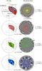 |
Fig. 5 3D and 2D views of portions of the star filtered at different frequencies. On the right, ASH results are represented in gray tones, and we have superimposed the path of the corresponding wave calculated by the method of raytracing. Only the radiative zone is represented. For ω = 0.2 mHz, the green dotted circle represents the outer turning point, and the green arrows highlight the nonpropagation region. For ω = 0.3 mHz, the two blue dotted circles represent the outer and inner turning points, and the blue arrow shows the nonpropagation region. For the four frequencies, the propagation regions correspond to the colored horizontal lines in Fig. 1. |
This manipulation allows us to highlight one of the main properties of IGWs. From the
linear theory of raytracing (Lighthill 1978; Gough 1993; Christensen-Dalsgaard 2011), we know that IGWs propagate along beams whose paths
are ruled by the dispersion relation (Eq. (2)). The shape formed by the beams at the point of the wave’s excitation is
called a St Andrew’s cross (Lighthill 1986; Voisin 1991). The wave’s energy is radiated around an
angle αth to the radial direction such that
 (4)where
N1 is the value of N in the region considered.
This angle is visible in Panels (D1)−(D3) of Fig. 4. To measure it,
we calculate its tangent in each panel using the relation
(4)where
N1 is the value of N in the region considered.
This angle is visible in Panels (D1)−(D3) of Fig. 4. To measure it,
we calculate its tangent in each panel using the relation 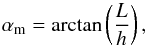 (5)where
L is the
length considered along the longitudinal direction and h along the radial
direction. For the measurement of L, we have translated the longitude from radians to
solar radii. The values found are indicated in Table 1 and compared to pseudo-theroretical values calculated from Eq. (4), where the value of N1 must be
deduced from the figure.
(5)where
L is the
length considered along the longitudinal direction and h along the radial
direction. For the measurement of L, we have translated the longitude from radians to
solar radii. The values found are indicated in Table 1 and compared to pseudo-theroretical values calculated from Eq. (4), where the value of N1 must be
deduced from the figure.
For αm, the main source of error is the measurement of the distances h and L. The error shown here corresponds to the width of the beam. For αth, we also considered an error coming from the measure of N1, which depends on the estimation of the starting point of the cross. Another possible source of error could be the quality of the filter, but since it has a very narrow bandwidth, this is negligible compared to the other factors.
This comparison shows that we find a bias between both values, where αm is systematically larger. A future work will be dedicated to exploring more frequencies, in order to determine the extent of this difference precisely and to decide on the precision of the linear dispersion relation used here. We have already checked that the influence of the coriolis acceleration is too weak at this rotation rate to explain the observed difference, even though it goes in the right direction.
3.2. Visualization of the high frequency wave pattern
We now apply this method of filtering to a larger portion of the star to see if we can
visualize other patterns than the quasi-circular spiral visible in Figs. 2a and b. Our results are shown in Fig. 5, in 3D and 2D views. To understand the results, we
computed the paths in 2D of some IGWs using the method of raytracing. It consists in
calculating the value of the wave’s phase along a path x(t) by resolving the
Hamiltonian system 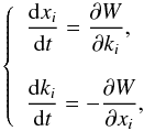 (6)where
W(x,k,t)
= ω, and (xi,ki)
the Cartesian coordinates of the position vector x and the
wavevector k (e.g., Lignières 2011). In our case, we employed polar coordinates, transforming the
system (10)into
(6)where
W(x,k,t)
= ω, and (xi,ki)
the Cartesian coordinates of the position vector x and the
wavevector k (e.g., Lignières 2011). In our case, we employed polar coordinates, transforming the
system (10)into 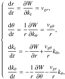 (7)where
vg =
vgrer
+
vgθeθ
is the group velocity of the wave at which the ray propagates. In this work, we use the
raytracing theory in 2D, as employed by many other authors (e.g., Lignières 2011; Christensen-Dalsgaard
2011; Kosovichev 2011), as a tool for
understanding our simulations. When computing the ray paths shown in Fig. 5, we used the Brunt-Väisälä frequency profile presented
in Fig. 1. Further developments of this method and
its generalization in 3D will be the object of a future work (Mathis et al., in prep.).
(7)where
vg =
vgrer
+
vgθeθ
is the group velocity of the wave at which the ray propagates. In this work, we use the
raytracing theory in 2D, as employed by many other authors (e.g., Lignières 2011; Christensen-Dalsgaard
2011; Kosovichev 2011), as a tool for
understanding our simulations. When computing the ray paths shown in Fig. 5, we used the Brunt-Väisälä frequency profile presented
in Fig. 1. Further developments of this method and
its generalization in 3D will be the object of a future work (Mathis et al., in prep.).
The results shown in Fig. 5 illustrate the diversity of the paths followed by the different waves. The lower the frequency, the more the ray paths look like spirals. Another way to understand it is to say that we retrieve the cross shape at the point of departure of the waves, whose angle α with the radial direction decreases with increasing frequency. In particular, the yellow case (ω = 0.05 mHz) is the closest to the general pattern (Figs. 2a and b). We thus confirm that what we see without filtering in the external region of the radiative zone is a sample of low-frequency waves. The other paths were not visible in Figs. 2a and b because the low-frequency part of the spectrum is dominant in amplitude (red tones in Fig. 2d). By filtering out this part, we can visualize the region of propagation of the other waves, and especially of the resonant g-modes.
The dispersion relation (Eq. (2)) imposes that the wave frequencies ω are less than the Brunt-Väisälä frequency N. Consequently, we can define the limit of the propagation region by two turning points rin and rout such that N(rin) = N(rout) = ω. For instance, the wave oscillating at 0.3 mHz (bottom panel of Fig. 5) is confined more deeply in the radiative zone than the one at 0.05 mHz (top panel). This is also visible in Fig. 1, where we indicate the regions of propagation of the waves shown in this section by colored lines. We note that the outer turning point is different from the penetration depth rov, where convective plumes deposit the energy transferred to waves. We clarify the different radii defined here in Fig. 6.
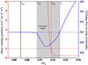 |
Fig. 6 Representation of the overshoot region defined between rc, the first zero of the enthalpy flux, and the point rov below which the amplitude of the flux drops to 10% of its most negative value. The radius rbcz corresponds to the point where the mean entropy gradient changes sign. The green vertical line represents the positions of rout for ω = 0.2 mHz. |
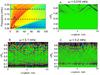 |
Fig. 7 Distinction between progressive and standing waves. The top left panel is a zoom of Fig. 2d (same colorbar). Three horizontal dotted lines represent the frequencies chosen in Panels A)−C). In these panels, we show the radial velocity in the same region filtered at three different frequencies. Low-frequency waves are rapidly damped and cannot form g-modes (Panel A)). In contrast, for ω = 0.1 mHz and ω = 0.2 mHz (Panels B) and C)), we see modes oscillating between the two turning points (white lines). |
It is interesting to see that, although the excitation region is located at the base of the convection zone (penetration region), the perturbation is able to propagate in a “non-propagation region” (blue arrow and limits materialized by green and blue dotted circles). This phenomenon can explain the fact that high-frequency modes ([0.3−0.4] mHz) are less powerful in the spectrum (Fig. 2d). In fact, a part of the initial energy transfered from the convective region to the waves is lost in the evanescent region, between the overshoot region and rout.
A moving version of Fig. 5 shows that the paths visible here do not propagate. They oscillate at the chosen frequency (wavefronts propagate toward the surface at the phase velocity), but the envelope remains stable. Thus, what we see here are stationary modes instead of progressive waves. In the following section, we show that the method of frequency filtering allows us to distinguish between these two families.
3.3. Distinguishing between progressive and standing waves
Along their propagation, IGWs are affected by a damping process that is proportional to
the radiative diffusivity of the fluid. In the linear and asymptotic (ω ≪ N)
approximations (Zahn et al. 1997), the amplitude of
a gravity wave propagating in a nonadiabatic medium is damped by a factor e− τ/
2 where ![Mathematical equation: \begin{equation} \label{eq:tau} \tau\left(r,\ell,\omega\right) = \left[\ell(\ell+1)\right]^{\frac{3}{2}}\int_{r}^{{\hat r}_{\rm out}}\kappa\frac{N^3}{\omega^4}\frac{\mathrm dr'}{r'^3} \cdot \end{equation}](/articles/aa/full_html/2015/09/aa26250-15/aa26250-15-eq74.png) (8)We see that this depends
on the radiative diffusivity coefficient κ, but also on both the frequency ω and the degree
ℓ. We
introduce
(8)We see that this depends
on the radiative diffusivity coefficient κ, but also on both the frequency ω and the degree
ℓ. We
introduce  ,
the maximum radius, close to the external turning point rout (with
,
the maximum radius, close to the external turning point rout (with
 ),
until when the JWKB approximation used to derive this expression can be assumed (see Fig.
6 and the detailed discussion in Appendix B and in
Alvan et al. 2013).
),
until when the JWKB approximation used to derive this expression can be assumed (see Fig.
6 and the detailed discussion in Appendix B and in
Alvan et al. 2013).
We know that g-modes are formed by positive interferences between two progressive IGWs. This implies that the amplitude of these IGWs is high enough to reach the inner turning point rin and then to go back toward the surface (see Eq. (B.8)).
In Fig. 7 we show the result of different filtering of the same region of the star. This is a slice of the equatorial plane (θ = π/ 2) with the normalized radius as vertical axis and the longitude ϕ as horizontal axis. In the top righthand panel, we zoom in to the lower region of the spectrum presented in Fig. 2. We see that, at ω = 0.016 mHz, the energy is fairly concentrated below the black line. The result is that the waves propagate over a finite distance before being completely damped. We draw the reader’s attention to the vertical axis that stops at 0.45 R⊙ since no wave is visible beyond. In contrast, for ω = 0.1 mHz and ω = 0.2 mHz, the main energy of the spectrum is above the black line (red tones), and in the real space, we clearly see that waves propagate between both turning points (white lines). They are excited at the top of the radiative zone, they go from rout to rin where they bounce, and they come back to rout.
We also note that the path of propagation changes between panels. In particular, the
inclination of the rays steepens with higher frequency following the tendency discussed in
Sect. 3.1. Moreover, we see that the number of rays
increases with ω. We can define an effective wavenumber
ℓeff by 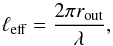 (9)where rout is the
outer turning point, and λ a wavelength that can be measured in the figures.
We find ℓeff ≈
11 for ω =
0.1 mHz and ℓeff ≈ 14 for ω = 0.2 mHz.
(9)where rout is the
outer turning point, and λ a wavelength that can be measured in the figures.
We find ℓeff ≈
11 for ω =
0.1 mHz and ℓeff ≈ 14 for ω = 0.2 mHz.
The conclusion of this study is to confirm the intuition that the spectrum realized in our 3D simulations is made up of both standing modes and progressive waves, as one expects. Since the radiative damping is more efficient for high values of ℓ, the corresponding waves do not have enough energy to bounce at their inner turning point and to form modes. They thus stay simple progressive IGWs. Although not discussed here in detail, it is clear that viscosity will also damp the waves (in addition to radiative diffusion), since we have a Prandtl number close to one in the radiative zone (Vadas & Fritts 2005).
3.4. Energy concentrated in planes
We now focus on a propagation property of IGWs in 3D. The results of this part highlight
the importance of studying gravity waves in fully spherical geometry. The asymptotic
theory of stellar oscillations (e.g., Gough 1993;
Christensen-Dalsgaard 2003; Aerts et al. 2010) predicts that in the case where we can neglect the
rotation of the star with respect to the waves frequencies (ω ≪ 2Ω0), the
horizontal components of the wavevector verify 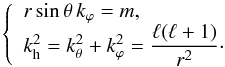 (10)Using
this property, Gough (1993) has shown theoretically
that the ray paths of waves defined by (ℓ,m) are confined in planes forming an angle
(10)Using
this property, Gough (1993) has shown theoretically
that the ray paths of waves defined by (ℓ,m) are confined in planes forming an angle
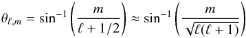 (11)with
the polar plane3. These planes do not depend on the
frequency of the waves, and they are independent of the dispersion relation. For instance,
this means that this property is also true for acoustic waves. We show an example in Fig.
8, where we have represented the planes where modes
(ℓ = 9,m =
0,3,5,9) are
expected to be concentrated. We see that the highest values of m correspond to planes
close to the equator. By definition, the m = 0 plane always contains the poles (axisymmetric
case).
(11)with
the polar plane3. These planes do not depend on the
frequency of the waves, and they are independent of the dispersion relation. For instance,
this means that this property is also true for acoustic waves. We show an example in Fig.
8, where we have represented the planes where modes
(ℓ = 9,m =
0,3,5,9) are
expected to be concentrated. We see that the highest values of m correspond to planes
close to the equator. By definition, the m = 0 plane always contains the poles (axisymmetric
case).
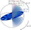 |
Fig. 8 Schematic representation of the propagation planes of azimuthal components of mode ℓ = 9. |
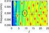 |
Fig. 9 Zoom of the spectrum represented in Fig. 2d. The dotted lines represent the bandwidth of the filter applied (Gaussian function centered at 0.3 mHz with full width at half maximum σ = 2 × 10⁻³ mHz) that allows us to select the mode ℓ = 9 in particular. |
We are going to test this theoretical result with our 3D nonlinear simulations. To
illustrate it, we use the result of a filtering at frequency 0.3 mHz. The corresponding
region in the spectrum is represented in Fig. 9. We
show a zoom of Fig. 2d and indicate the bandwidth of
the filter. The mode located in the middle of this bandwith is ℓ = 9. We here recall that
the spectrum shown includes all values of m (see Eq. (3)). As a consequence, the red peaks of energy visible in this figure are formed
by the superposition of all m components, whose frequency ωn,ℓ,m is slightly
shifted by the effect of the rotation. This rotational splitting is given by 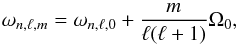 (12)where
ωn,ℓ,0 is the central
peak, corresponding to m =
0 (see Sect. 4.3.2 of Alvan et al.
2014).
(12)where
ωn,ℓ,0 is the central
peak, corresponding to m =
0 (see Sect. 4.3.2 of Alvan et al.
2014).
Knowing the rotation rate of our model (1Ω⊙) and the frequency considered here, the distance ωn,ℓ,m − ωn,ℓ,0 between two peaks of different m and same ℓ is much less than the one between two modes of consecutive n values (see Alvan et al. 2014). That is why we do not see any overlap in the peak and why the filter selects the whole azimuthal components of the mode.
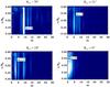 |
Fig. 10 Results of Fourier transforms applied to four selected planes of the radiative zone, after a frequency filtering at ω = 0.3 mHz. The main value of m in each plane corresponds to the one expected by the asymptotic theory. The horizontal axis is voluntarily extended up to m = 30 to show that we only retrieve the expected values of m. |
After having filtered the whole radiative zone, we need to access each plane of the sphere and to measure the corresponding dominant azimuthal number m. For example, to reach the plane θ9,5 = 31 (represented in green in Fig. 8), we apply a rotation matrix of angle 90 − θ9,5 to the sphere, so that the desired plane is now located at the equator. We then apply a Fourier transform with respect to the longitude ϕ to obtain the spectrum in m. The result for four planes is given in Fig. 10. The white zones correspond to the dominant values of m.
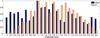 |
Fig. 11 Distribution of the energy transported by the IGWs as a function of the latitude for two different models. The vertical axis is normalized by the maximum value. |
We see that these values are indeed different for each plane and that they correspond to those expected by the theory. In particular, the m = 9 peak is clearly dominant in the θ9,9 plane and so is m = 0 in the θ9,0 plane. That secondary peaks are also visible can be explained by the following arguments. First, for the top lefthand panel (θ9,9), we notice two weak peaks at m = 12 and m = 14. We assigned them to the mode ℓ = 14, which is partially taken into account by the filter (see Fig. 9). Nevertheless, it is clear that the m = 9 mode is dominant. Then, the theory predicted that the existence of these planes assumes some approximation that is not verified by our model. The adiabatic approximation made by Gough (1993) is not true here since our waves are submitted to thermal and viscous diffusivities. This could result in a leakage of the energy from one plane to another. Moreover, the presence of rotation in our model is to be considered as a small disturbance. Indeed, by using our 3D raytracing code (Mathis et al., in prep.), we have shown that the propagation of IGWs in planes is no longer verified in the case of rapidly rotating stars (except for m = 0). Finally, we can invoke numerical noise because our spherical harmonic transform uses a finite number of mesh points, which results in a leakage of the energy from one pair (ℓ,m) to another. Despite these limitations, this is a clear example of the need to model those waves in full spherical geometry.
In Alvan et al. (2014), we showed that the energy of a given g-mode tends to concentrate in high m components. We clarify this result in Fig. 11 by showing the distribution of energy as a function of latitude for the current model (turb2) and for a less turbulent model discussed in detail in that paper. Indeed, we see that for the model ref, the energy is concentrated around the equator. We suspect that this concentration of energy may be due to the shape of convection (banana cells) in low-latitude regions. If we increase the turbulence of the convection (model turb2), the distribution becomes more homogeneous in latitude, but we still see a peak around the equator (colatitude θ = π/ 2).For instance, this could imply a more efficient transport of angular momentum induced by the presence of IGWs in the equatorial regions.
4. Conclusion
The aim of this paper has been to understand gravity waves in solar-like stars. To this end, we analyzed our 3D simulations in order to deepen our understanding of the complexity of the spectrum excited. Here, we have explored and described the substructures of this spectrum by showing the co-existence of both progressive IGWs and standing modes. For the first time in simulation, we were able to visualize individual IGWs in the inner regions of the stars.
-
−
Thanks to our frequency filtering method, we isolated somewell-chosen waves in spectral space and shown that their energypaths in the real space correspond to the one predicted by the linearraytracing theory.
-
We showed that it is possible to distinguish between g-modes and progressive IGWs by measuring their damping rate. If the damping rate is too high, IGWs do not reach their inner turning point (whose depth depends on the frequency of the wave), and they cannot form resonant mode. In contrast, we see in the figures that isolated waves taken in the high part of the spectrum (high frequency and/or high degree ℓ) can bounce at r = rin and form a g-mode. The cut-off frequency separating g-modes and progressive IGWs scales with
![Mathematical equation: \hbox{$\left[\ell\left(\ell+1\right)\right]^{3/8}$}](/articles/aa/full_html/2015/09/aa26250-15/aa26250-15-eq111.png) .
This analysis gives us precise knowledge of the composition of the spectrum excited in
our model. Consequently, it gives a rather good understanding of the same processes
acting on the real wave spectrum of the Sun.
.
This analysis gives us precise knowledge of the composition of the spectrum excited in
our model. Consequently, it gives a rather good understanding of the same processes
acting on the real wave spectrum of the Sun. -
Our third result consists in the study of the spatial distribution of the waves energy in the 3D radiative zone. We have shown that, according to the theoretical predictions of Gough (1993), waves of different degrees ℓ and azimuthal order m are distributed differently in space. Their energy is confined in planes, whose inclination with the polar direction varies with (ℓ,m). The plane that is the closest to the equator is the one with m = ℓ. Moreover, as noted in Alvan et al. (2014), the waves associated to high values of m have the highest amplitude, which may be explained by studying the repartition of convective plumes. This result for the concentration of energy in planes is very important because it could guide our research into g-modes at the surface of the Sun and our understanding of the angular momentum transport by gravity waves.
It is important to highlight that, to perform these simulations, we adopted values of diffusivities that are necessarily much higher than their microscopic values. For this reason, some of the predictions of the model (e.g., concerning the energetical aspects of the spectrum of IGWs excited by convection) must be considered with caution.
The direct perspectives of this work are to improve our analysis by taking the effect of rotation that modifies the ray paths and break the propagation in planes into account. This project requires improving both the simulation (exploring other parameter regimes) and the theory. Indeed, our analysis is guided by the results of the raytracing theory but also by theoretical results about the impact of rotation on the excitation and propagation of IGWs (Belkacem et al. 2009; Mathis et al. 2014). We also plan to study the nonlinear aspects of IGWs, including for example triadic interactions or wave breaking (e.g., Staquet & Sommeria 2002; Barker 2011; Bourget et al. 2013). Finally, the extension of this study to other types of stars is in progress and will provide a new source of asteroseismic predictions.
Another hypothesis for explaining the solid body rotation of the solar radiative zone relies on the existence of a buried large-scale fossil magnetic field, whose existence and effect are still the subject of debates in the community (Gough & McIntyre 1998; Strugarek et al. 2011; Acevedo-Arreguin et al. 2013).
The exact expression found by Gough (1993) is the one using ℓ + 1 / 2, because he employed a general formalism that is different from the usual projection on spherical harmonics followed by the asymptotic approximation. Nevertheless, with respect to the precision of our results, the approximation  is largely acceptable for the degree of the mode chosen here, ℓ = 9.
Acknowledgments
We thank the referee, A. Barker, for his constructive comments that allowed us to improve the article. We are grateful to N. Featherstone, B. Brown, and D. Lecoanet for useful discussions. We acknowledge funding by the ERC grant STARS2 207430 (www.stars2.eu), the European Communitys Seventh Framework Program ([FP7/2007-2013]) under the grant agreements no. 312844 (SPACEINN) and no. 269194 (IRSES/ASK), and the CNRS Physique théorique et ses interfaces program. The simulations were performed using HPC resources of GENCI 1623 and PRACE 1069 projects.
References
- Acevedo-Arreguin, L. A., Garaud, P., & Wood, T. S. 2013, MNRAS, 434, 720 [NASA ADS] [CrossRef] [Google Scholar]
- Aerts, C., Christensen-Dalsgaard, J., & Kurtz, D. D. W. 2010, Asteroseismology, Astron. Astrophys. Lib. (London: Springer, Limited) [Google Scholar]
- Alvan, L., Mathis, S., & Decressin, T. 2013, A&A, 553, A86 [NASA ADS] [CrossRef] [EDP Sciences] [Google Scholar]
- Alvan, L., Brun, A. S., & Mathis, S. 2014, A&A, 565, A42 [NASA ADS] [CrossRef] [EDP Sciences] [Google Scholar]
- Appourchaux, T., Belkacem, K., Broomhall, A.-M., et al. 2010, A&ARv, 18, 197 [NASA ADS] [CrossRef] [Google Scholar]
- Barker, A. 2011, MNRAS, 414, 1365 [NASA ADS] [CrossRef] [Google Scholar]
- Barker, A., & Ogilvie, G. I. 2010, MNRAS, 404, 1849 [NASA ADS] [Google Scholar]
- Belkacem, K., Mathis, S., Goupil, M. J., & Samadi, R. 2009, A&A, 508, 345 [NASA ADS] [CrossRef] [EDP Sciences] [Google Scholar]
- Berry, M. V., & Mount, K. E. 1972, Rep. Progr. Phys., 35, 315 [NASA ADS] [CrossRef] [Google Scholar]
- Booker, J., & Bretherton, F. 1967, J. Fluid Mech., 27, 513 [NASA ADS] [CrossRef] [Google Scholar]
- Bourget, B., Dauxois, T., Joubaud, S., & Odier, P. 2013, J. Fluid Mech., 723, 1 [NASA ADS] [CrossRef] [Google Scholar]
- Braginsky, S. I., & Roberts, P. H. 1995, Geophys. Astrophys. Fluid Dynamics, 79, 1 [Google Scholar]
- Brown, B. P., Vasil, G. M., & Zweibel, E. G. 2012, ApJ, 756, 109 [Google Scholar]
- Browning, M., Brun, A. S., & Toomre, J. 2004, ApJ, 601, 512 [NASA ADS] [CrossRef] [Google Scholar]
- Brummell, N. H., Clune, T. L., & Toomre, J. 2002, ApJ, 570, 825 [Google Scholar]
- Brun, A. S., Antia, H. M., Chitre, S. M., & Zahn, J.-P. 2002, A&A, 391, 725 [NASA ADS] [CrossRef] [EDP Sciences] [Google Scholar]
- Brun, A. S., Miesch, M. S., & Toomre, J. 2004, ApJ, 614, 1073 [NASA ADS] [CrossRef] [Google Scholar]
- Brun, A. S., Miesch, M. S., & Toomre, J. 2011, ApJ, 742, 79 [NASA ADS] [CrossRef] [Google Scholar]
- Charbonnel, C., & Talon, S. 2005, Science, 309, 2189 [NASA ADS] [CrossRef] [PubMed] [Google Scholar]
- Charbonnel, C., Decressin, T., Amard, L., Palacios, A., & Talon, S. 2013, A&A, 554, A40 [NASA ADS] [CrossRef] [EDP Sciences] [Google Scholar]
- Christensen-Dalsgaard, J. 2011, Lect. Notes Phys., 1025 [Google Scholar]
- Christensen-Dalsgaard, J. 2003, Stellar Oscillations [Google Scholar]
- Clune, T., Elliott, J., Miesch, M. S., Toomre, J., & Glatzmaier, G. A. 1999, Parallel Computing, 25, 361 [Google Scholar]
- Dintrans, B., Brandenburg, A., Nordlund, Å., & Stein, R. F. 2005, A&A, 438, 365 [NASA ADS] [CrossRef] [EDP Sciences] [Google Scholar]
- Fritts, D. C., & Alexander, M. J. 2003, Rev. Geophys., 41, 1003 [Google Scholar]
- Fuller, J., Lecoanet, D., Cantiello, M., & Brown, B. 2014, ApJ, 796, 17 [Google Scholar]
- Garcia, R., Jiménez, A., Mathur, S., et al. 2008, Astron. Nachr., 329, 476 [Google Scholar]
- Garcia, R. 2009, Highlight of Astronomy (HoA), Proc. JD-11, IAU 2009 XXVII general assembly, meeting held in Rio de Janeiro, Brazil, 15, 345 [Google Scholar]
- Garcia, R. A., Turck-Chièze, S., Jiménez-Reyes, S. J., et al. 2007, Science, 316, 1591 [NASA ADS] [CrossRef] [PubMed] [Google Scholar]
- Garcia Lopez, R. J., & Spruit, H. C. 1991, ApJ, 377, 268 [NASA ADS] [CrossRef] [Google Scholar]
- Glatzmaier, G. A. 1984, J. Comput. Phys., 55, 461 [Google Scholar]
- Gostiaux, L., Didelle, H., Mercier, S., & Dauxois, T. 2007, Exp Fluids, 123 [Google Scholar]
- Gough, D. 1993, in Astrophysical Fluid Dynamics − Les Houches 1987, 399 [Google Scholar]
- Gough, D. O., & McIntyre, M. E. 1998, Nature, 394, 755 [NASA ADS] [CrossRef] [Google Scholar]
- Hurlburt, N. E., Toomre, J., & Massaguer, J. M. 1986, ApJ, 311, 563 [NASA ADS] [CrossRef] [Google Scholar]
- Hurlburt, N. E., Toomre, J., Massaguer, J. M., & Zahn, J.-P. 1994, ApJ, 421, 245 [NASA ADS] [CrossRef] [Google Scholar]
- Kiraga, M., Jahn, K., Stepien, K., & Zahn, J.-P. 2003, Acta Astron., 53, 321 [NASA ADS] [Google Scholar]
- Kiraga, M., Stepien, K., & Jahn, K. 2005, Acta Astron., 55, 205 [NASA ADS] [Google Scholar]
- Kosovichev, A. G. 2011, Lect. Notes Phys., eds. J.-P. Rozelot, & C. Neiner (Berlin, Heidelberg: Springer Berlin Heidelberg), 832 [Google Scholar]
- Kumar, P., Talon, S., & Zahn, J.-P. 1999, ApJ, 520, 859 [NASA ADS] [CrossRef] [Google Scholar]
- Lantz, S. R. 1992, Ph.D. Thesis, Cornell University [Google Scholar]
- Lecoanet, D., & Quataert, E. 2013, MNRAS, 430, 2363 [NASA ADS] [CrossRef] [Google Scholar]
- Lee, U., Neiner, C., & Mathis, S. 2014, MNRAS, 443, 1515 [NASA ADS] [CrossRef] [Google Scholar]
- Lighthill, J. 1978, Waves in Fluids (Cambridge: Cambridge University Press) [Google Scholar]
- Lighthill, J. 1986, Provided by the SAO/NASA Astrophysics Data System [Google Scholar]
- Lignières, F. 2011, in Lect. Notes Phys. (Berlin, Heidelberg: Springer), 259 [Google Scholar]
- Massaguer, J. M., Latour, J., Toomre, J., & Zahn, J.-P. 1984, A&A, 140, 1 [NASA ADS] [Google Scholar]
- Mathis, S., Decressin, T., Eggenberger, P., & Charbonnel, C. 2013, A&A, 558, A11 [NASA ADS] [CrossRef] [EDP Sciences] [Google Scholar]
- Mathis, S., Neiner, C., & Tran Minh, N. 2014, A&A, 565, A47 [NASA ADS] [CrossRef] [EDP Sciences] [Google Scholar]
- Miesch, M. S., Elliott, J. R., Toomre, J., et al. 2000, ApJ, 532, 593 [NASA ADS] [CrossRef] [Google Scholar]
- Montalban, J. 1994, A&A, 281, 421 [NASA ADS] [Google Scholar]
- Mowbray, D. E., & Rarity, B. S. H. 1967, J. Fluid Mech., 28, 1 [NASA ADS] [CrossRef] [Google Scholar]
- Pantillon, F. P., Talon, S., & Charbonnel, C. 2007, Arxiv e-prints [arXiv:0708.1477v1] [Google Scholar]
- Perrard, S., Le Bars, M., & Le Gal, P. 2013, in Lect. Notes Phys. (Berlin, Heidelberg: Springer), 239 [Google Scholar]
- Press, W. H. 1981, ApJ, 245, 286 [NASA ADS] [CrossRef] [Google Scholar]
- Provost, J., & Berthomieu, G. 1986, A&A, 165, 218 [NASA ADS] [Google Scholar]
- Rogers, T. M., & Glatzmaier, G. A. 2005, ApJ, 620, 432 [NASA ADS] [CrossRef] [Google Scholar]
- Rogers, T. M., Glatzmaier, G. A., & Jones, C. A. 2006, ApJ, 653, 765 [NASA ADS] [CrossRef] [Google Scholar]
- Saikia, E., Singh, H. P., Chan, K. L., Roxburgh, I. W., & Srivastava, M. P. 2000, ApJ, 529, 402 [NASA ADS] [CrossRef] [Google Scholar]
- Schatzman, E. 1993, A&A, 279, 431 [NASA ADS] [Google Scholar]
- Staquet, C., & Sommeria, J. 2002, An. Rev. Fluid Mech., 34, 559 [Google Scholar]
- Strugarek, A., Brun, A. S., & Zahn, J.-P. 2011, A&A, 532, A34 [NASA ADS] [CrossRef] [EDP Sciences] [Google Scholar]
- Talon, S., & Charbonnel, C. 2005, A&A, 440, 981 [NASA ADS] [CrossRef] [EDP Sciences] [Google Scholar]
- Talon, S., & Charbonnel, C. 2008, A&A, 482, 597 [NASA ADS] [CrossRef] [EDP Sciences] [Google Scholar]
- Unno, W., Osaki, Y., Ando, H., Saio, H., & Shibahashi, H. 1989, Nonradial oscillations of stars, 2nd edn. (Tokyo: University of Tokyo Press) [Google Scholar]
- Vadas, S. L., & Fritts, D. C. 2005, J. Geophys. Res. Atm., 110, 15103 [NASA ADS] [CrossRef] [Google Scholar]
- Voisin, B. 1991, J. Fluid Mech., 231, 439 [NASA ADS] [CrossRef] [Google Scholar]
- Zahn, J.-P. 1991, A&A, 252, 179 [NASA ADS] [Google Scholar]
- Zahn, J.-P., Talon, S., & Matias, J. 1997, A&A, 322, 320 [Google Scholar]
Appendix A: ASH code and 3D model description
The ASH code solves the set of 3D anelastic hydrodynamic equations in a spherical geometry. The equations are fully nonlinear in velocity, and we linearize the thermodynamic variables with respect to a spherically symmetric and evolving mean state. We denote ,  ,
,  , and
, and  as the reference density, pressure, temperature, and specific entropy. Fluctuations in this reference state are denoted by ρ, P, T, and S. We assume a linearized equation of state
  (A.1)and the zeroth-order ideal gas law
  (A.2)where γ is the first adiabatic exponent, cp the specific heat per unit mass at constant pressure, and ℛ the gas constant.
We also introduce the local velocity  expressed in spherical coordinates (r,θ,ϕ) in the frame rotating at constant angular velocity Ω0 = Ω0ez. The set of hydrodynamic equations solved by ASH in the present case is
 ![Mathematical equation: \appendix \setcounter{section}{1} \begin{eqnarray} \label{eq:3} \left\{ \begin{array}{ll} \hbox{ (a) }&\vec\nabla.\left(\bar\rho\vec {{{v}}}\right) = 0 \hbox{,} \\ \hbox{ (b) }&\bar\rho\left(\displaystyle\frac{\partial \vec {{{v}}}}{\partial t} + \left(\vec {{{v}}}.\vec\nabla\right)\vec {{{v}}}\right) = -\bar{\rho}\vec\nabla\widetilde\omega -\bar{\rho}\displaystyle\frac{S}{c_p}\vec{g} - 2\bar\rho \vec\Omega_0 \times \vec {{{v}}} \\ &\hbox{\hspace{1cm}}- \vec\nabla . {\mathcal{D}} -\left[\vec\nabla\bar{{P}} - \bar\rho\vec{{g}}\right] \hbox{,}\\ \\ \hbox{ (c) }& \bar\rho \bar{{T}}\displaystyle\frac{\partial {S}}{\partial t}\! +\! \bar\rho\bar{{T}}\vec{{{v}}}.\vec\nabla\left({S}+\bar{{S}}\right)= \bar\rho \epsilon \!+ \!\vec\nabla . \left[ \kappa_{\rm r}\bar\rho c_p \vec\nabla\left({T}+\bar{{T}}\right) \right.\\ \end{array} \right. \end{eqnarray}](/articles/aa/full_html/2015/09/aa26250-15/aa26250-15-eq128.png) (A.3)where Eq. (A.3a) is the continuity equation in the anelastic approximation; (A.3b) the momentum equation; and (A.3c) the energy equation.
(A.3)where Eq. (A.3a) is the continuity equation in the anelastic approximation; (A.3b) the momentum equation; and (A.3c) the energy equation.
We define the gravitational acceleration g, the viscous stress tensor  defined by
  (A.4)with
  the strain rate tensor and δij the Kronecker symbol. The bracketed term on the righthand side of the momentum equation is initially zero since the system begins in hydrostatic balance. For this equation, we used the Lantz-Braginsky-Roberts (LBR) form (e.g., Lantz 1992; Braginsky & Roberts 1995) advocated by Brown et al. (2012), who have shown that the classical anelastic formulation may introduce a bias in the conservation of energy, in the case of strongly stably stratified atmospheres. In this formulation, we use the reduced pressure
  instead of the fluctuating pressure P and neglect the buoyancy term
  associated with the non-adiabatic reference state in the radiative zone. Thus, the new buoyancy term
  only contains the contribution of entropy fluctuations, and the contribution due to pressure perturbations is included in the reduced pressure gradient. In the energy Eq. (A.3c), κr is the radiative diffusivity based on a 1D solar structure model, and ν and κ are effective diffusivities modeling momentum and heat transport by subgrid-scale (SGS) motions that are unresolved by the simulation. Their profiles are represented in Fig. A.1.
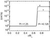 |
Fig. A.1 Radial profiles of the effective diffusivities κ (thermal) and ν (viscous). The model used here is called turb2 in Alvan et al. (2014). |
The diffusivity κ0 is also part of the SGS treatment in the convective zone and is chosen such that the entropy flux carries the solar flux outward at the top of the domain. It is negligible in the radiative zone (Miesch et al. 2000). Finally, the volume heating term  represents the energy generation by nuclear burning with ϵ = ϵ0Tk. The constant ϵ0 is set such that the radially integrated heating term equals the solar luminosity at the base of the convection zone, and k = 9 allows us to take both contributions of the p-p chains and CNO cycles into account (Brun et al. 2002).
The computational domain extends from rbot = 0 to rtop = 0.97 R⊙ where R⊙ = 6.9599 × 1010 cm is the solar radius. The boundary conditions at the top of the domain are torque-free velocity conditions and constant heat flux (Brun et al. 2011). The inner boundary conditions are chosen to deal with the central singularity at rbot = 0. Conditions on the poloidal and toroidal components of the mass flux impose that only ℓ = 1 mode can go through the center, and thermal condition are also adapted. This treatment is explained in detail in Alvan et al. (2014).
In the model presented here, the spatial resolution is Nr × Nθ × Nϕ = 1581 × 512 × 1024, with a non-uniform radial grid chosen to resolve the turbulent convection, the oscillations of IGWs in the radiative zone, and the steep drop of diffusivities at the interface between both zones (Alvan et al. 2014).
The 3D simulation is initialized using a reference state derived from a 1D solar structure model (Brun et al. 2002). The set of Eqs. (A.3)is then solved in expanding the velocity and thermodynamic variables in spherical harmonics Yℓ,m(θ,ϕ) for their horizontal structure and using a fourth-order finite-difference approach on a nonuniform grid for their radial part. For the time integration, we use an explicit Adams-Bashforth scheme for the advection and Coriolis terms and a semi-implicit Crank-Nicolson treatment for the diffusive and buoyancy terms (Glatzmaier 1984; Clune et al. 1999). The reference state is updated during the simulation with the spherically averaged perturbation fields.
After a few convective overturning times, a balance is established between the contributions to the total flux of the different physical processes (Brun et al. 2011; Alvan et al. 2014). It allows us to see that the convective flux becomes negative at the base of the convective zone, which is the signature of the overshoot process (e.g., Zahn 1991), where downflows penetrate the radiative zone slightly owing to their inertia. This induces a perturbation in velocity and temperature at the top of the radiative zone, which propagates in the form of a gravity wave. With the bulk excitation process (Lecoanet & Quataert 2013), overshoot is responsible for the excitation of IGWs in solar-like stars.
Appendix B: Understanding the cut-off frequency between modes and progressive waves
The goal of this appendix is to derive the dependence of the cut-off frequency that separates modes and progressive waves, ωc, on their latitudinal degree (ℓ).
We develop the radial component of the velocity on spherical harmonics:  (B.1)Next, we get from the system formed by the linearized momentum, continuity, and heat transport equations in the adiabatic case
 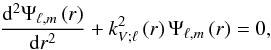 (B.2)where
 , and
, and 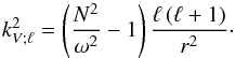 (B.3)From then on, we focus on the low-frequency asymptotic regime in which ω ≪ N. We follow Zahn et al. (1997) by applying the JWKB and the quasi-adiabatic approximations that allows us to derive the expression for ur;ℓ,m:
 ![Mathematical equation: \appendix \setcounter{section}{2} \begin{eqnarray} u_{r;\ell,m}&=&A_{\ell,m}r^{-\frac{3}{2}}{\overline\rho}^{-\frac{1}{2}}\left(\frac{N^2}{\omega^2}\right)^{-\frac{1}{4}}P_{l}^{\vert m\vert}\left(\cos\theta\right)\nonumber\\ &&\times\cos\left(\omega t+m\varphi\pm\int_{r}^{{\hat r}_{\rm out}}k_{V;\ell}{\rm d}r'\right)\exp\left[-\frac{\tau\left(r,\ell,\omega\right)}{2}\right], \label{eq:urlm} \end{eqnarray}](/articles/aa/full_html/2015/09/aa26250-15/aa26250-15-eq159.png) (B.4)where Aℓ,m is an amplitude coefficient, which includes the normalization of spherical harmonics, and
(B.4)where Aℓ,m is an amplitude coefficient, which includes the normalization of spherical harmonics, and  are the associated Legendre polynomials. We recall the radiative damping expression (Eq. (8))
 ![Mathematical equation: \appendix \setcounter{section}{2} \begin{equation} \tau\left(r,\ell,\omega\right) = \left[\ell(\ell+1)\right]^{\frac{3}{2}}\int_{r}^{{\hat r}_{\rm out}}\kappa\frac{N^3}{\omega^4}\frac{\mathrm dr'}{r'^3}\cdot \end{equation}](/articles/aa/full_html/2015/09/aa26250-15/aa26250-15-eq162.png) (B.5)Since the JWKB approximation falls at the two turning points
(B.5)Since the JWKB approximation falls at the two turning points  , we introduce the two radius (
 , with
  and ) between which it can be applied (see the detailed discussion in Berry & Mount 1972; and Alvan et al. 2013).
Then, we derive the horizontally averaged kinetic energy of IGWs using results derived by Zahn et al. (1997):  (B.6)where ⟨···⟩θ,ϕ = 1 / 4π∫θ,ϕsinθdθdϕ. Using Eq. (B.4), it becomes
 ![Mathematical equation: \appendix \setcounter{section}{2} \begin{equation} E_{K;\ell,\rm m}\left(r\right)=\frac{1}{4}A_{\ell,m}^2\frac{N}{\omega}\left<\left[P_{l}^{\vert m\vert}\left(\cos\theta\right) \right]^2 \right>_ {\theta} r^{-3}\exp\left[-{\tau\left(r,\ell,\omega\right)}\right]. \label{eq:kinE} \end{equation}](/articles/aa/full_html/2015/09/aa26250-15/aa26250-15-eq168.png) (B.7)We then define the cut-off frequency that separates modes and progressive waves with the following criterion:
(B.7)We then define the cut-off frequency that separates modes and progressive waves with the following criterion:  (B.8)When K ≪ 1, the wave has lost a large part of its kinetic energy and cannot reflect to form a standing mode. Using Eq. (B.7), it becomes
 ![Mathematical equation: \appendix \setcounter{section}{2} \begin{equation} \exp\left[-\tau\left({\hat r}_{\rm in},\ell,\omega\right)\right]=K\frac{N\left({\hat r}_{\rm out}\right){\hat r}_{\rm out}^{-3}}{N\left({\hat r}_{\rm in}\right){\hat r}_{\rm in}^{-3}}=\alpha. \end{equation}](/articles/aa/full_html/2015/09/aa26250-15/aa26250-15-eq171.png) (B.9)Assuming that
(B.9)Assuming that  and vary weakly with ωc for ωc ≪ N, we finally obtain
 ![Mathematical equation: \appendix \setcounter{section}{2} \begin{equation} \omega_{\rm c}\approx\left[-\frac{\displaystyle\int_{{\hat r}_{\rm in}}^{{\hat r}_{\rm out}}\kappa N^3\frac{\mathrm dr'}{r'^3}}{\ln\alpha} \left[\ell(\ell+1)\right]^{\frac{3}{2}}\right]^{\frac{1}{4}}\equiv\beta\left[\ell\left(\ell+1\right)\right]^{\frac{3}{8}} \end{equation}](/articles/aa/full_html/2015/09/aa26250-15/aa26250-15-eq174.png) (B.10)as observed in power spectrum of our direct 3D nonlinear ASH simulations (Fig. 2).
(B.10)as observed in power spectrum of our direct 3D nonlinear ASH simulations (Fig. 2).
All Tables
All Figures
|
Fig. 1 Profile of the Brunt-Väisälä frequency as a function of the normalized radius. Colored horizontal lines highlight the regions of propagation of the waves revealed by our filtering technique in Fig. 5. |
| In the text | |
|
Fig. 2 a) 3D rendering of the simulated star. We represent the radial velocity divided by its rms value at each radius. b) Equatorial slice. Like in the 3D view, IGWs pattern are visible in the inner radiative zone as quasi-circular spirals. c) rms profiles of the total (solid line) and radial (dotted line) velocities as a function of the normalized radius, averaged over longitude, latitude, and time (about 10 convective overturning times). d) Energy spectrum of gravity waves computed at r0 = 0.5 R⊙ as a function of degree ℓ and frequency ω. Ridges are formed by g-modes of same radial order n, and we see that they tend to the maximum Brunt-Väisälä frequency at high order ℓ (dotted white line). The black solid line denotes the separation between g-modes (above) and progressive waves (below). |
| In the text | |
|
Fig. 3 Percentage of the total energy (squared radial velocity) distributed in standing and progressive gravity waves. |
| In the text | |
|
Fig. 4 Filtering of the same image at three different frequencies. Downflows are represented in blue, upflows in red tones. A) Selected zone of the star. B) and C) frequency spectra of points B) and C) where we see one or two main peaks. The vertical axis represents the normalized radial velocity. The vertical red line indicates the position of the Gaussian filter (width = 2 × 10⁻⁴ mHz). D1), D2) and D3): result of the filtering of image A) at three frequencies. Wave beams are visible with an inclination that varies with the frequency, forming St Andrew’s crosses. The angles’ values are indicated in Table 1. |
| In the text | |
|
Fig. 5 3D and 2D views of portions of the star filtered at different frequencies. On the right, ASH results are represented in gray tones, and we have superimposed the path of the corresponding wave calculated by the method of raytracing. Only the radiative zone is represented. For ω = 0.2 mHz, the green dotted circle represents the outer turning point, and the green arrows highlight the nonpropagation region. For ω = 0.3 mHz, the two blue dotted circles represent the outer and inner turning points, and the blue arrow shows the nonpropagation region. For the four frequencies, the propagation regions correspond to the colored horizontal lines in Fig. 1. |
| In the text | |
|
Fig. 6 Representation of the overshoot region defined between rc, the first zero of the enthalpy flux, and the point rov below which the amplitude of the flux drops to 10% of its most negative value. The radius rbcz corresponds to the point where the mean entropy gradient changes sign. The green vertical line represents the positions of rout for ω = 0.2 mHz. |
| In the text | |
|
Fig. 7 Distinction between progressive and standing waves. The top left panel is a zoom of Fig. 2d (same colorbar). Three horizontal dotted lines represent the frequencies chosen in Panels A)−C). In these panels, we show the radial velocity in the same region filtered at three different frequencies. Low-frequency waves are rapidly damped and cannot form g-modes (Panel A)). In contrast, for ω = 0.1 mHz and ω = 0.2 mHz (Panels B) and C)), we see modes oscillating between the two turning points (white lines). |
| In the text | |
|
Fig. 8 Schematic representation of the propagation planes of azimuthal components of mode ℓ = 9. |
| In the text | |
|
Fig. 9 Zoom of the spectrum represented in Fig. 2d. The dotted lines represent the bandwidth of the filter applied (Gaussian function centered at 0.3 mHz with full width at half maximum σ = 2 × 10⁻³ mHz) that allows us to select the mode ℓ = 9 in particular. |
| In the text | |
|
Fig. 10 Results of Fourier transforms applied to four selected planes of the radiative zone, after a frequency filtering at ω = 0.3 mHz. The main value of m in each plane corresponds to the one expected by the asymptotic theory. The horizontal axis is voluntarily extended up to m = 30 to show that we only retrieve the expected values of m. |
| In the text | |
|
Fig. 11 Distribution of the energy transported by the IGWs as a function of the latitude for two different models. The vertical axis is normalized by the maximum value. |
| In the text | |
|
Fig. A.1 Radial profiles of the effective diffusivities κ (thermal) and ν (viscous). The model used here is called turb2 in Alvan et al. (2014). |
| In the text | |
Current usage metrics show cumulative count of Article Views (full-text article views including HTML views, PDF and ePub downloads, according to the available data) and Abstracts Views on Vision4Press platform.
Data correspond to usage on the plateform after 2015. The current usage metrics is available 48-96 hours after online publication and is updated daily on week days.
Initial download of the metrics may take a while.