| Issue |
A&A
Volume 581, September 2015
|
|
|---|---|---|
| Article Number | A77 | |
| Number of page(s) | 13 | |
| Section | Stellar structure and evolution | |
| DOI | https://doi.org/10.1051/0004-6361/201526154 | |
| Published online | 07 September 2015 | |
KIC 9533489: a genuine γ Doradus – δ Scuti Kepler hybrid pulsator with transit events
1 Konkoly Observatory, MTA CSFK, Konkoly Thege M. u. 15-17, 1121 Budapest, Hungary
e-mail: This email address is being protected from spambots. You need JavaScript enabled to view it.
2 Koninklijke Sterrenwacht van België, Ringlaan 3, 1180 Brussel, Belgium
3 Astrophysics Group, Keele University, Staffordshire ST5 5BG, UK
4 Astronomy Department, University of California, Berkeley, CA 94720, USA
5 NASA Exoplanet Science Institute/Caltech, Pasadena, CA 91125, USA
6 Center for Exoplanets and Habitable Worlds, The Pennsylvania State University, University Park, PA 16802, USA
7 Departamento de Física Teórica y del Cosmos, Universidad de Granada, Campus de Fuentenueva, 18071 Granada, Spain
Received: 22 March 2015
Accepted: 4 June 2015
Abstract
Context. Several hundred candidate hybrid pulsators of type A–F have been identified from space-based observations. Their large number allows both statistical analyses and detailed investigations of individual stars. This offers the opportunity to study the full interior of the genuine hybrids, in which both low radial order p- and high-order g-modes are self-excited at the same time. However, a few other physical processes can also be responsible for the observed hybrid nature, related to binarity or to surface inhomogeneities. The finding that most δ Scuti stars also show long-period light variations represents a real challenge for theory.
Aims. We aim at determining the pulsation frequencies of KIC 9533489, to search for regular patterns and spacings among them, and to investigate the stability of the frequencies and the amplitudes. An additional goal is to study the serendipitously detected transit events: is KIC 9533489 the host star? What are the limitations on the physical parameters of the involved bodies?
Methods. We performed a Fourier analysis of all the available Kepler light curves. We investigated the frequency and period spacings and determined the stellar physical parameters from spectroscopic observations. We also modelled the transit events.
Results. The Fourier analysis of the Kepler light curves revealed 55 significant frequencies clustered into two groups, which are separated by a gap between 15 and 27 d-1. The light variations are dominated by the beating of two dominant frequencies located at around 4 d-1. The amplitudes of these two frequencies show a monotonic long-term trend. The frequency spacing analysis revealed two possibilities: the pulsator is either a highly inclined moderate rotator (v ≈ 70 km s-1, i> 70°) or a fast rotator (v ≈ 200 km s-1) with i ≈ 20°. The transit analysis disclosed that the transit events that occur with a ≈197 d period may be caused by a 1.6 RJup body orbiting a fainter star, which would be spatially coincident with KIC 9533489.
Key words: techniques: photometric / stars: individual: KIC 9533489 / stars: variables: delta Scuti / planets and satellites: detection / stars: oscillations
© ESO, 2015
1. Introduction
Recently, ultra-precise photometric data from three space missions revolutionised the field of variable star studies: the Canadian MOST satellite (Walker et al. 2003), the French-led CoRoT mission (Auvergne et al. 2009), and the NASA mission Kepler (Koch et al. 2010). The almost continuous, high-precision single-band light curves allow the detection of many pulsation frequencies with amplitudes down to the micromagnitude level. All these missions provide an enormous amount of extremely high-quality data for analysis, enabling advanced asteroseismic studies for many years to come. On the other hand, we still need complementary ground-based data for an unambiguous interpretation of the light variations observed by space telescopes, for instance, to determine the physical parameters and modal content of the pulsators, or to identify the (mostly non-eclipsing) binary or multiple systems.
A large part of intermediate-mass (1.2–2.5 M⊙) A and F spectral type stars shows pulsations in the intersecting region of the main sequence and the classical instability strip in the Hertzsprung–Russell diagram (HRD). Among others, we find here δ Scuti (δ Sct) variables, pulsating in low radial order p- and mixed p-g-modes with periods in the 0.01−0.3 d range, and γ Doradus (γ Dor) pulsators with high-order g-modes in the 0.3−3 d period range. The δ Sct pulsations are excited by the κ mechanism operating in the HeII partial ionisation zone (see e.g. the review by Breger 2000), while the γ Dor pulsations are driven by the convective blocking mechanism operating at the base of the convection zone (Guzik et al. 2000). The instability regions of these two mechanisms overlap in the HRD, and hybrid δ Sct – γ Dor pulsators were first predicted (Dupret et al. 2004) and then confirmed (Henry & Fekel 2005). We refer to these as hybrids hereafter. The simultaneously excited p- and g-modes provide information on the envelope and the region near the core of the star. Therefore, these hybrids are very important targets for asteroseismic investigations. However, it is difficult to find them with ground-based observations because the γ Dor pulsations usually have low amplitudes, and their typical frequencies, close to 1–2 d-1, are strongly affected by the daily aliasing, as well as by atmospheric effects and instrumental drifts.
Thanks to the recent space-based observations, we now have hundreds of stars classified as A–F-type hybrid candidates (see e.g. Uytterhoeven et al. 2011; Hareter 2012). This allows both statistical analyses and detailed investigations of individual stars. The most striking result of the preliminary analyses of the hybrid candidates is that they are not confined to the theoretically predicted intersecting region of the two pulsation types. Instead, they occur everywhere in the δ Sct domain (Grigahcène et al. 2010; Uytterhoeven et al. 2011), and it seems that practically all δ Sct stars show low-frequency light variations (Balona 2014). In the case of the hotter δ Sct pulsators (Teff > 7500 K), the presumed existence of hybrid pulsations challenges the theory of stellar pulsations, because we do not expect that the convective blocking mechanism can operate in the thin convective upper layer (Balona 2014). Furthermore, most of the candidates show frequencies between about 5 and 10 d-1, even though this region has formerly been considered as a frequency gap, at least for low spherical degree (l = 0−3) modes (see Fig. 2 of Grigahcène et al. 2010). This observational finding could be explained by the combined effects of frequency shifts of high-order g-modes caused by the Coriolis force, detection of high-spherical-degree modes, and rotational splitting (Bouabid et al. 2013).
Which mechanisms are responsible for the simultaneous occurrence of low- and high-frequency variations revealed in so many A–F-type stars? Different possible scenarios have to be considered:
-
1.
Genuine δ Sct–γ Dor hybrids: both δ Sct and γ Dor-type pulsations are self-excited in these objects. About a dozen such confirmed objects have been investigated in detail, but there must be many more genuine hybrids among the known candidates.
-
2.
Eclipsing or ellipsoidal binaries: the object might be a δ Sct pulsator in an eclipsing or ellipsoidal binary system. The long periodicity in the light variations corresponds to the orbital period or half of it, depending on the case. The physical parameters of the binary components can be derived independently of any theoretical (asteroseismic) assumption. These parameters can be used as constraints for subsequent asteroseismic investigations.
-
3.
Tidal excitation: a δ Sct star in a close, eccentric binary, where the external tidal forces excite g-mode pulsations (Willems & Aerts 2002). HD 209295 is an example (Handler et al. 2002).
-
4.
Stellar rotation coupled with surface inhomogeneities: these can also cause detectable signals in the low-frequency region. Low-temperature spots may be an obvious explanation, but mechanisms generating such features are not expected to operate in normal (non-Ap, non-Am) A-type stars, since their convective layers are thin and thus likely have weak magnetic fields. Nevertheless, statistical investigation of Kepler A-type stars (Balona 2011) shows that the low-frequency variability could be caused by rotational modulation in connection with starspots or other corotating structures. Low-temperature spots cause characteristic light-curve variations. One low-frequency signal and several of its harmonics are expected in the Fourier spectrum. However, finite starspot lifetimes and/or differential rotation combined with spot migration result in a number of significant peaks around the rotational frequency on longer time scales.
However, in the case of KIC 5988140, none of these simple scenarios could explain the observations in a fully satisfactory way (Lampens et al. 2013). Indeed, in this case, the scenario of binarity has been discarded on the basis of the double-wave pattern of the radial velocity curve mimicking the pattern of the light curve (after pre-whitening of the higher frequencies). The other two remaining scenarios explaining the low frequencies in terms of g-mode pulsation or rotational modulation are also problematic since the predicted light-to-velocity amplitude ratio based on two simple spotted surface models is 40 times higher than observed.
KIC 9533489 is another Kepler hybrid candidate investigated by Uytterhoeven et al. (2011) and was found to be an exotic case: in addition to its confirmed hybrid character, we also detected a few transit events in the Kepler light curve. In the following sections, we present the results of the frequency analyses and derived (physical and pulsational) properties of this object, as well as a possible model for the transit events detected in the light curve.
2. Kepler data
KIC 9533489 (Kp = 12.96 mag, α2000 = 19h38m41.7s, δ2000 = + 46d07m21.6s) was observed both in long-cadence (LC) and short-cadence (SC) mode. The LC data have a sampling time of 29.4 min (Jenkins et al. 2010), while the SC observations provide a brightness measurement every 58.85 s (Gilliland et al. 2010). We used the raw flux data of KIC 9533489 available from the Kepler Asteroseismic Science Operations Center (KASOC) database. We analysed the LC data of 17 quarters of Kepler observations (Q1–Q17, 13 May 2009–11 May 2013) and the SC data of 3 quarters (Q1, Q5.1–3, Q6.1–3, 13 May 2009–22 September 2010). The contamination level of the measurements is estimated to be only 1.6 per cent.
The strong long-term instrumental trends present in the light curves were removed before analysis. First, we divided the time strings into segments. These segments contain gaps no longer than 0.1–0.5 d. Then, we separately fitted and subtracted cubic splines from each segment. We used one knot point for every 1000 (SC data) or 100–200 points (LC data) to define the splines. We omitted the obvious outliers and the data points affected by the transit events. The resulting SC and LC light curves consist of 307 950 and 62 418 data points, spanning 498 (with a large gap) and 1450 days, respectively.
3. Spectroscopy
For an unambiguous interpretation of the results of the light-curve analysis, the atmospheric stellar parameters must be known, that is, the effective temperature (Teff), surface gravity (log g), and projected rotational velocity (v sin i). Therefore, we observed KIC 9533489 in the 2013 and 2014 observing seasons with the High Efficiency and Resolution Mercator Echelle Spectrograph (HERMES, Raskin et al. 2011) attached to the 1.2 m Mercator Telescope, with the FIbre-fed Echelle Spectrograph (FIES) at the 2.5 m Nordic Optical Telescope (NOT), and also with the INTEGRAL instrument (Arribas et al. 1998) using the 4.2 m William Herschel Telescope (WHT). All instruments are located at the Roque de los Muchachos Observatory (ORM, La Palma, Spain). We also acquired data with the High Resolution Echelle Spectrometer (HIRES, Vogt et al. 1994) attached to the 10 m Keck I telescope (W. M. Keck Observatory, Hawaii, US). Table 1 shows the journal of the spectroscopic observations.
Log of spectroscopic observations of KIC 9533489.
We obtained the reduced spectra from the dedicated pipelines of the HERMES, FIES, and HIRES instruments, while the single-order WHT spectrum centred on Hα was reduced using IRAF1 routines. All spectra were corrected for barycentric motion, then combined into a single averaged spectrum per instrument.
Although the signal-to-noise ratio (S/N) of the averaged HERMES spectrum is low (S/N = 20 per wavelength bin at λ ~ 500 nm), we were able to derive the radial velocity (RV) for that epoch by calculating a cross-correlation function with an F0-star synthetic spectrum, excluding regions of Balmer and telluric lines. We performed the same procedure on the FIES and HIRES spectra, too. We found that the RV measurements are consistent with each other within the errors, pointing to a value of 6.5 ± 1.5 km s-1. That is to say, the star showed no sign of RV change over a period of ~330 days, and therefore cannot be considered a multiple system.
Because it has a sufficiently high S/N and covers a wide wavelength domain that contains all the majour Balmer lines, we started to derive the star’s astrophysical parameters on the FIES averaged spectrum. We estimated v sin i by adopting the Fourier transform (FT) approach (for an overview, see Gray 1992; Royer 2005, and references therein). To increase the S/N and to limit the effect of blends, the FT was performed on an average line profile obtained through cross-correlation of the spectrum with an F0 mask from which we excluded the strongest lines. The result shows that the star is probably a moderate rotator (see Table 3).
We estimated Teff by fitting the Hα, Hβ, Hγ, and Hδ line profiles of the FIES spectrum. The continuum normalisation of the spectrum was realised in three steps. A first normalisation was done with the IRAF continuum task to perform a very preliminary determination of Teff and log g in the 400–450 nm range (metallicity was kept solar and microturbulence was fixed to 2 km s-1). The fit was realised by using the girfit program based on the minuit minimisation package and by interpolating in a grid of synthetic spectra. These synthetic spectra and corresponding LTE model atmospheres were computed with the computer codes synspec (Hubeny & Lanz 1995, and references therein) and atlas9 (Castelli & Kurucz 2004, and references therein), respectively. They were then convolved with the rotational profile and with a Gaussian instrument profile to account for the resolution of the spectrograph. The observations were then divided by the closest not normalised synthetic spectrum.
After being sigma clipped to remove most mismatch features, the resulting curve was divided into two to four smaller regions that were smoothened with polynomials of degrees 5 to 10. The observed spectrum was divided by the resulting function (see Fig. 1 of Frémat et al. 2007 for an illustration of the procedure), then normalised with the IRAF continuum task and a low-order spline. Regions around Hα, Hβ, Hγ, and Hδ were then isolated and fitted separately. Because hydrogen lines below 8000 K are only sensitive to effective temperature, all other parameters were kept fixed, and we tried to exclude most metal lines from the fit as best possible. Each time, three to five different starting points were chosen between 6000 and 8000 K, which resulted in a median value and an inter-quantile dispersion of 7350 ± 200 K.
The same procedure was then applied on the other spectra, except that fewer hydrogen lines were available. We list the values we obtained in Table 2, where the last column details the hydrogen lines that we considered. For the HERMES and FIES spectra the error bars were deduced from the scatter of our different determinations and trials, while for the INTEGRAL and HIRES determinations we adopted the numerical value provided by the minuit package when it computes the covariance matrix. The final Teff value was obtained by combining these different estimated into a rounded mean whose error is provided by the largest deviation (see Table 3).
Effective temperature values derived from the fit of the hydrogen line profiles observed with different instruments.
Stellar parameters of KIC 9533489, determined from spectroscopic observations (“spectra”) and evolutionary tracks and isochrones (“models”, Girardi et al. 2000).
Since our initial scope was not to perform a detailed chemical abundance analysis, we derived the metal content by scaling the abundance of all elements heavier than boron by the same factor, which we call here “metallicity”. For this purpose we studied the region between 496 and 564 nm. To identify the features that are the most sensitive to surface gravity, we considered two synthetic spectra of the same effective temperature (7200 K) and v sin i, but with different extreme log g values (3.5 and 5.0). The difference between the two spectra only exceeds the limits given by the S/N of the observed spectra in the region around the Mg I triplet (515 to 520 nm). We then constructed a first regular grid of synthetic spectra for different values of the microturbulent velocity and metallicity. The χ2 value between the observations and the spectra of each (vmic, metallicity) node was computed from 496 to 564 nm, excluding the 515–520 nm part. Finally, a Levenberg-Marquardt minimisation algorithm was applied around the minimum, and a covariance matrix was computed to estimate the error bars by interpolating in a second grid of spectra with smaller steps in metallicity and microturbulence. Log g was then derived by fixing the microturbulence and metallicity to the best values found in the previous step and by applying the Levenberg-Marquardt algorithm to the region between 515–520 nm. Because the final log g value did not have any significant effect on the agreement between the synthetic spectrum and observations in the other considered wavelength domains, we stopped the process.
Part of the HIRES spectrum is shown in Fig. 1, where it is compared to the synthetic spectrum that results from our atmospheric parameter determination procedure. The residuals between the two spectra are also plotted in the same figure. These residuals are higher than the S/N. We checked therefore for any trace of an additional contribution in the spectrum, as suggested by the transit modelling (see Sect. 6).
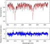 |
Fig. 1 Observed HIRES spectrum (in black) and synthetic model (in red) of an F0-type star with v sin i = 70 km s-1 over the wavelength range 400–455 nm. The residual spectrum is drawn in blue. |
First, we computed the cross-correlation of the FIES spectrum with a G5 spectral template. We did not find any evidence of absorption lines due to a cooler companion. This could mean that the presumed companion’s contribution to the total light is too low to be detected in the spectrum and/or that its spectral lines are too broadened (i.e. due to rotation or/and macroturbulence). A light factor corresponding to Δm = 2.25 mag might explain such a non-detection.
We next computed an (F0+G5) composite model spectrum and examined the variance between this model and the HIRES spectrum in the wavelength range 500–560 nm for a wide range of possible radial velocities. The G5 synthetic spectrum was computed assuming v sin i = 10 km s-1. The minimum variance was found around 31 km s-1, that is, it is different from the radial velocity of the Kepler star. This second test might hint at the existence of an additional stellar object, but we remain unable to directly identify the lines of the transit host in the spectrum.
Table 3 summarises the stellar parameters derived from the spectra. Knowing the values of Teff and log g and assuming a solar metallicity, we estimated the mass, luminosity, radius, and age of KIC 9533489 (see also Table 3) by applying the evolutionary tracks and isochrones from Girardi et al. (2000). The Teff and log g values indicate that KIC 9533489 is situated in the overlapping region of the δ Sct and γ Dor observational instability strips (see e.g. Fig. 10 of Uytterhoeven et al. 2011). The age estimation suggests a young object, located near the zero-age main sequence (ZAMS), but the uncertainty is very large (Fig. 2).
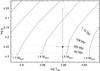 |
Fig. 2 Location of KIC 9533489 on the surface gravity vs. effective temperature diagram. Evolutionary tracks for 1.4, 1.5, 1.6, and 1.7 M⊙, as derived by Girardi et al. (2000) are plotted with solid lines. Dotted lines show 63 Myr –1.12 Gyr isochrones. |
4. Adaptive optics observations
We obtained near-infrared adaptive optics (AO) images of KIC 9533489 in the Br-γ (2.157 μm) filter using the NIRC2 imager behind the natural guide star adaptive optics system at the Keck II telescope on 04 September 2014. Data were acquired in a three-point dither pattern to avoid the lower left corner of the NIRC2 array, which is noisier than the other three quadrants. The dither pattern was performed three times with step sizes of 3″, 2.5″, and 2.0″ for a total of nine frames; individual frames had an integration time of 30 s. The individual frames were flat-fielded, sky-subtracted (sky frames were constructed from a median average of the nine individual source frames), and co-added.
The average AO-corrected seeing was FWHM = 0.048″; the pixel scale of the NIRC2 camera is 10 mas/pixel. 5σ sensitivity limits were determined for concentric annuli surrounding the primary targets; the annuli were stepped in integer multiples of the FWHM with widths of 1 FWHM. The sensitivity achieved reached Δmag ≈ 8 mag at 0.2″ separation from the central target star in the band of observation. Using typical stellar Kepler-infrared colours (Howell et al. 2012), this value translates into the Kepler bandpass to be about Δmag ≈ 10−11 mag.
One source was detected approximately 1.1″ to the west of the primary target (Δα = 1.12 ± 0.005″; Δδ = 0.09 ± 0.005″; Fig. 3). The companion is 3.412 ± 0.014 mag fainter than the target at 2.2 μm; by deblending the 2MASS Ks photometry, we find the infrared brightnesses of the target and the companion to be Ks = 12.055 ± 0.020 mag and Ks = 15.467 ± 0.024 mag. No observations in other wavelengths were obtained, but based upon the typical Kepler-infrared colours (Howell et al. 2012), the companion has a Kepler bandpass magnitude of Kp = 17.9 ± 0.8 mag; thus, the companion is ≳5 mag fainter than the primary target and contributes less than 1% to the Kepler light curve.
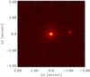 |
Fig. 3 Keck II adaptive optics image of KIC 9533489. |
5. Frequency analysis
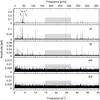 |
Fig. 4 Fourier transforms of the original SC light curve and of the light curve pre-whitened for 2, 9, 46, and 63 frequencies. The blue dashed lines denote the 4 ⟨ A ⟩ significance level, where ⟨ A ⟩ is calculated as the moving average of radius 8 d-1 of the pre-whitened spectrum. The frequency gap between ≈15 and 27 d-1 is indicated with a grey band. The vertical dotted line denotes the Nyquist limit of the LC data. |
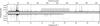 |
Fig. 5 Fourier transforms of the original SC (upper panel) and LC (bottom panel) light curve. The frequency gap between ≈15 and 27 d-1 found in the SC data is indicated with a grey band. The vertical dotted line denotes the Nyquist limit of the LC data. Red lines connect the lowest and highest frequency peaks of the SC data with their Nyquist aliases detected in the LC Fourier transform. |
We performed the Fourier analysis of both the SC and LC data sets and compared the frequencies. The increased sampling of the SC data allows directly determining pulsation frequencies above the LC Nyquist limit (fLC,Nyq = 24.5 d-1, fSC,Nyq = 734 d-1). The LC observations, having a longer time base, provide better frequency resolution and allow investigating the long-term frequency stability. The Rayleigh frequency resolutions of the long- and short-cadence data sets are fLC,R = 0.0007 and fSC,R = 0.002 d-1, respectively.
We performed a standard successive pre-whitening of the light curves for significant signals using Period04 (Lenz & Breger 2005) and SigSpec (Reegen 2007). The results were also checked with the photometry modules of famias (Zima 2008). The frequencies obtained were consistent within the errors using the different programs. Figure 4 presents the Fourier transforms of the original and the pre-whitened SC data sets. We stopped the process when none of the remaining peaks reached the threshold of S/N ≈ 4 (Breger et al. 1993). Altogether, 63 frequencies were determined in this way. We also checked the spectral significances (sig) of the frequencies, as derived by SigSpec. All of the peaks were found to be above the default threshold value for determining frequencies (5.46, see Reegen 2007). The lowest amplitude peaks have sig ~ 8 (cf. Table 4). We checked which of these frequencies was also found in the LC data. Below the LC Nyquist limit, we found all but eight frequencies. All of the eight missing frequencies are below 1 d-1. Both the instrumental effects in the original data (see e.g. Murphy 2012) and the correction method were applied to remove these affects in this low-frequency region. Therefore, we excluded these eight peaks from the list of accepted frequencies. We checked the remaining significant frequencies using the Kepler Data Characteristics Handbook (KSCI-19040-004) and found none of them to be of instrumental origin.
We note that the frequencies detected in the SC data above the LC Nyquist limit, except for the three lowest amplitude frequencies, also appear in the LC data. These can be identified as Nyquist aliases at fi,LC = 2fLC,Nyq−fi,SC, split by Kepler’s orbital frequency (Murphy et al. 2013). Figure 5 presents the FT of the original SC and LC data. We can detect both real pulsation frequencies and the Nyquist aliases above 11.3 d-1 in the Fourier transform of the LC light curve.
Table 4 lists the 55 accepted frequencies and the differences between the frequency values derived from the SC and LC data. They differ only in the fourth–sixth decimals. We note that the frequency difference (0.0056 d-1) of the closest peaks (f16 and f51) is 2.8 times larger than the Rayleigh frequency resolution of the SC data set, which means that all of the identified frequencies are well-resolved.
Two closely spaced peaks at ≈4 d-1 (f1 and f2) dominate the light variation of KIC 9533489 (see Fig. 6). Most of the peaks (42) are below 15 d-1, and 27 of these are below 5 d-1. The rest of the frequencies (13) are in the 27–38 d-1 range. There is a clear frequency gap between 15 and 27 d-1. We indicate this region with a grey band in Figs. 4 and 5. These gaps play an important role in hybrid star studies because they allow distinguishing between different mode-driving mechanisms.
We checked the frequencies for possible combination terms (kfi or pfi ± qfj). Considering test results on simulated light curves (Pápics 2012), we restricted our search to the second-order combinations, that is, | p | = 1 and | q | = 1. We accepted a peak as a combination if the amplitudes of both parent frequencies were larger than that of their presumed combination term, and the difference between the observed and the predicted frequency was not larger than the Rayleigh resolution of the SC data (0.002 d-1). This way, we found one harmonic peak (f49 = 2f2) and 11 other combination terms. Although f30 is close to 2f1, it does not fulfil this criterion. We indicate the combination terms in Table 4. In addition to the combinations consisting of independent parent frequencies, we list two cases in parentheses in Table 4. These are equal to two and four times the value of f28, respectively, which is itself a combination of two large-amplitude frequencies (f28 = f2−f3). It is not clear yet whether this is a coincidence or whether f28 (0.84 d-1) has a particular importance for some unknown reason.
Frequency content of the KIC 9533489 Kepler data.
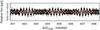 |
Fig. 6 Section of the SC light curve of KIC 9533489 and the fit of the two dominant frequencies (red line). The plot exhibits the beating effect that dominates the light variations. |
5.1. Stability investigations
Strong amplitude variability on month- and year-long timescales was reported in the A–F-type hybrid KIC 8054146 (Breger et al. 2012). We also examined the long-term stability of the most dominant peaks. We used the LC data set because it spans a much longer time interval than the SC data. We investigated the nine highest amplitude frequencies below the LC Nyquist limit. First, we calculated the actual frequencies and their amplitudes for each quarter (Q1–Q17). Then, we determined  values that characterise the observed variability of these parameters as the deviation of the quarterly data points from their time-averages, relative to the uncertainties of the measurements. We did not detect variability in any of the nine frequencies, as
  for each of them.
However, this test revealed the variability of two amplitudes. We obtained values for the amplitudes of the two most dominant frequencies, f1 and f2, of 8.3 and 4.8, respectively. The value of the other seven amplitudes remained below 1.5. Figure 7 presents the amplitude values of f1 and f2 for Q1–Q17. The amplitudes show a linear trend and vary similarly, but in opposite directions. The continuous lines are linear fits to the data points, which show a 2.4 and 2.0 per cent relative amplitude variation per year. The  values for the linear fits are 1.1 and 0.6 for f1 and f2, respectively. These amplitude changes could be explained in terms of energy exchange between the two dominant modes and interpreted as coupling.
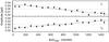 |
Fig. 7 Amplitudes of f1 and f2 in the different light-curve segments of the Q1–Q17 LC data. The dashed line shows the error-weighted average of the data points, the continuous line is a linear fit to the data. |
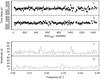 |
Fig. 8 Time delays calculated for the two dominant modes f1 and f2 (top panels), and their Fourier transform (bottom panels). |
We also checked whether we can detect any sign of phase modulation (PM) of the dominant modes by applying the method presented by Murphy et al. (2014). A periodic phase modulation would indicate the presence of a stellar or even a substellar companion of KIC 9533489. The panels of Fig. 8 show the time delays of f1 and f2, calculated from ten-day segments of the LC data, and their Fourier transforms, respectively. The formula used to calculate the time delays is  , where
  is the mean of the φj(t) phases derived from the different light-curve segments for a fixed νj frequency (Murphy et al. 2014). None of these point to any periodic variation, that is, KIC 9533489 is not a member of a 20 d <Porb< 4 yr binary system: neither the time delay plots nor the corresponding Fourier transforms have a common significant peak corresponding to a possible common orbital period.
5.2. Frequency and period spacings
If it is a genuine hybrid, KIC 9533489 will simultaneously show excited high-order g- and low-order p-modes. We therefore checked whether there are any regularities between the periods and frequencies in the presumed g- and p-mode regions, respectively, predicted by stellar pulsation theory. For references on the theoretical background of non-radial pulsations, see for example Tassoul (1980), Unno et al. (1989), and Aerts et al. (2010).
High radial order g-modes are excited in γ Dor pulsators. According to the first-order asymptotic approximation of non-radial stellar pulsations, the separation of consecutive overtones that have the same ℓ spherical harmonic index (ΔPℓ = Pn + 1,ℓ−Pn,ℓ) is  (1)where
 ![Mathematical equation: \begin{eqnarray*} \Pi_0= 2 \pi^2 \left[\int_{r_1}^{r_2} \frac{N}{r} {\rm d}r\right]^{-1}, \end{eqnarray*}](/articles/aa/full_html/2015/09/aa26154-15/aa26154-15-eq178.png) and N is the Brunt-Väisälä frequency. That is, period spacings are expected to be constant in a chemically homogeneous star, but inhomogeneities (rapid changes of the mean molecular weight in the transition zones) cause deviations from this constant value (see e.g. Miglio et al. 2008 and Bouabid et al. 2011). Following Eq. (1), the period spacing ratios for the different ℓ modes are
and N is the Brunt-Väisälä frequency. That is, period spacings are expected to be constant in a chemically homogeneous star, but inhomogeneities (rapid changes of the mean molecular weight in the transition zones) cause deviations from this constant value (see e.g. Miglio et al. 2008 and Bouabid et al. 2011). Following Eq. (1), the period spacing ratios for the different ℓ modes are 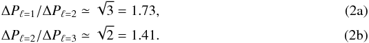 Even though the pulsation modes in low radial order p-modes are in the non-asymptotic regime for most of the δ Sct stars, we can still note a clustering of frequencies with the presumed large separation, Δνℓ = νn + 1,ℓ−νn,ℓ (see e.g. García Hernández et al. 2009 and Paparó et al. 2013). The large separation can be calculated in a first approximation as
 ![Mathematical equation: \begin{eqnarray*} \Delta \nu = 2 \left[\int_{r_1}^{r_2} \frac{{\rm d}r}{c_{\rm s}} \right]^{-1}, \end{eqnarray*}](/articles/aa/full_html/2015/09/aa26154-15/aa26154-15-eq182.png) where cs is the sound speed. The equation given for the large separation (integral over the inverse sound speed) is valid for high radial order p-modes (Tassoul 1980; Gough 1990). It was generalised in terms of the mean density of the stars by Suárez et al. (2014), based on numerical calculations using a huge model grid. The relation obtained for the δ Sct stars domain can be approximated by
where cs is the sound speed. The equation given for the large separation (integral over the inverse sound speed) is valid for high radial order p-modes (Tassoul 1980; Gough 1990). It was generalised in terms of the mean density of the stars by Suárez et al. (2014), based on numerical calculations using a huge model grid. The relation obtained for the δ Sct stars domain can be approximated by  (3)where Δν⊙ = 134.8 μHz and
  g cm-3.
Another well-known relation in the case of δ Sct pulsations is the frequency ratio of the radial fundamental and first-overtone radial mode (see Stellingwerf 1979):  (4)In high-overtone (n ≫ ℓ) modes and slow rotation, the frequency differences of the rotationally split components can be calculated by the asymptotic relation:
  (5)where the coefficient Cn,ℓ ≈ 1 /ℓ(ℓ + 1) for g-modes, Cn,ℓ ≈ 0 for p-modes, and Ω is the (uniform) rotation frequency. As δν ~ [1−1 /ℓ(ℓ + 1)], the ratio of the rotationally split ℓ = 1 and ℓ = 2g-modes in the case of equal δm is
  (6)We also have in a first approximation:
 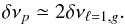 (7)We investigated the frequency set of KIC 9533489 considering these relations.
We note that for rapidly rotating stars, additional terms to Eq. (5) have to be considered in calculating rotationally split frequencies, considering higher order rotational effects. In this case, δνn,ℓ,m also depends on νn,ℓ and on m ( ). For a theoretical background, see Gough & Thompson (1990) and Kjeldsen et al. (1998) for the acoustic modes, and Chlebowski (1978) and Dziembowski & Goode (1992) for the g-modes. In Sect. 5.2.2, we use the simple form of Eq. (5) to derive a first approximation for the rotation period of the star.
5.2.1. Frequency ratios
By considering the modelling results of Suárez et al. (2014) on main-sequence δ Sct stars and knowing the mean density of KIC 9533489, we estimated the frequency of the theoretical radial fundamental mode. Taking into account the estimated radius and mass and their uncertainties (see Table 3), the mean density of the star normalised to the solar value may be between 0.2 and 0.6 ρ/ρ⊙. These values indicate that the radial fundamental mode could lie between ~13–23 d-1 (150–260 μHz), practically in the observed frequency gap, according to Fig. 2 of Suárez et al. (2014). This means that the radial fundamental mode is either f35 (14.58 d-1), the only mode between 13–23 d-1, or the radial modes are not exceeding the S/N = 4 significance level. There is no first- overtone frequency pair for f35 with a frequency ratio in the range of 0.77–0.78 according to Eq. (4).
As the radial fundamental mode represents the low-frequency limit for p-modes, we can assume that the frequencies below the gap (up to 14.6 d-1) are γ Dor-type g-modes. Rapid rotation may explain both the shifts of g-modes into higher frequencies than the classical γ Dor pulsation domain (Bouabid et al. 2013) and the lack of radial modes. Indeed, rapidly rotating δ Sct stars generally tend to show mainly non-radial modes of lower amplitude in comparison with the slow rotators (see e.g. Breger 2000). It is also possible that some of the observed frequencies above 5 d-1 are non-zonal (m ≠ 0) modes generated by rotational splittings.
5.2.2. Frequency spacings and stellar rotation
We studied the distribution of the frequencies by applying different methods: by calculating their Fourier transforms (see e.g. Handler et al. 1997), generating histograms of the frequency differences (e.g. in Matthews 2007), and using Kolmogorov-Smirnov (K-S) tests (Kawaler 1988). We defined and analysed several sets of frequencies: those below 5, 10, 15, and above 27 d-1. In the Fourier tests, we assigned an equal amplitude to all frequencies. Local maxima in the FTs indicate that characteristic spacings exist between the frequencies. In the K-S test, the quantity Q is defined as the probability that the observed frequencies are randomly distributed. Thus, any characteristic frequency spacing in the frequency spectrum should appear as a local minimum in Q. We present the results of these computations in Fig. 9.
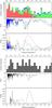 |
Fig. 9 Searching for characteristic frequency spacings. From top to bottom: histograms of frequency differences, results of K-S tests, Fourier transforms of different frequency sets. Red boxes/lines: frequencies below 5 d-1, green boxes/lines: frequencies below 10 d-1, blue boxes/lines: frequencies below 15 d-1, grey boxes/lines: frequencies above 27 d-1. |
Provided that both g- and p-modes occur, we expect to find periodicities that belong to rotationally split frequencies, according to Eqs. (5)–(7). However, we note that these relations are only valid for slow rotators, and in the case of KIC 9533489 (v sin i = 70 ± 7 km s-1), there might be deviations from the constant frequency spacings. Figure 9 indicates possible characteristic spacings in the range of 0.2–0.4, 1.0–1.4, and 2.0–2.7 d-1 in the low-frequency domain and in the range of 0.4–0.7 and 2.6–2.7 d-1 above 27 d-1 in the high-frequency domain.
We list the possible rotational periods of KIC 9533489 calculated using Eq. (5) for some specific spacings in Table 5. These values correspond to local maxima of the FT of the frequencies below 10 d-1 (green line in Fig. 9) or above 27 d-1. We also considered the possibility that in the case of a high inclination of the pulsation axis, or if any mode selection mechanism according to m is in operation, we may not detect the m = 0 components of the ℓ = 1 triplets, and the spacings belong to δm = 2 splittings. For completeness, we also list the possible rotational periods for ℓ = 2 modes. We assume that the pulsation and rotation axes coincide.
To check if the two dominant modes (f1 and f2) are rotationally split frequencies, we included their 0.44 d-1 separation in Table 5. Finally, we included the case of f34 (1.5622 d-1). It takes part in two combinations: f39 = f12 + f34 and f45 = f12−f34. This practically means that there is an equidistant triplet structure around f12 (6.3656 d-1), with a separation of the value of f34. There are no other similar structures found, but 1.56 d-1 is another frequency separation we have to take into account as the possible rotational spacing.
Possible rotational periods (P), equatorial velocities (v), and inclinations (i) of KIC 9533489 derived by applying different frequency spacing values.
According to Eq. (7), we expect that δνp ≃ 2δνℓ = 1,g. Considering the 0.37 and 0.66 d-1 characteristic spacings of the presumed g- and p-modes, these might correspond to rotational splitting values of ℓ = 1 modes. Another possibility is that the 1.30 and 2.67 d-1 spacings are caused by the stellar rotation.
None of these spacings selected in the g-mode region clearly shows the 0.6 ratio expected for ℓ = 1 and 2 modes (see Eq. (6)).
Using the rotation periods calculated from the different spacings, the estimated radius of the star, and the observed v sin i (see Table 3), we indicate for guidance the corresponding equatorial velocity (v) and inclination values in Table 5. This reveals that since the lower limit for v is ≈ 63 km s-1 (v sin i = 70−7 km s-1, i = 90°, cf. Table 3), the 0.37 d-1 separations of the presumed g-modes cannot be interpreted as rotational spacings. This also holds for the 0.66 d-1 spacing of the presumed p-modes, but not for the 0.44 d-1 frequency separation (cf. Table 5). Therefore 0.44 d-1 is a plausible rotational spacing.
The (critical) Keplerian velocity of vKep = 437 km s-1 is reached at an inclination of i = 9.4°. It seems improbable that the 2.37 d-1 spacing represents rotationally split ℓ = 1,δm = 1g-modes because the derived equatorial velocity of 371 km s-1 is more than 80 per cent of vKep.
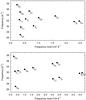 |
Fig. 10 Echelle diagrams of the 12 independent frequencies, supposed p-modes, above the frequency gap. |
The 2.67 d-1 spacing found from the high-frequency region requires further investigation. We have discussed already that it is a potential rotational spacing value. However, it can also be related to the large separation of frequencies. There are known cases in the literature for which such peaks in the Fourier transforms of the observed frequencies turned out to be at one half of the large separation (e.g. Handler et al. 1997; García Hernández et al. 2009). It is expected when modes with different ℓ values are observed. Suárez et al. (2014) presented a method for estimating the large separation (Δν) for δ Sct stars (Eq. (3)). For KIC 9533489 (ρ/ρ⊙ ≃ 0.4), the large separation is expected to be 68.6 μHz (5.9 d-1) according to their formula. Half of this value is 2.95 d-1, which is not far from the 2.67 d-1 spacing observed. Considering the uncertainties in the radius and mass determination and that equidistant spacings are expected for slow rotators and frequencies in the asymptotic regime, the 2.67 d-1 value is a reasonable estimate for half of the large separation.
We demonstrate in Fig. 10 that this 2.67 d-1 frequency spacing is not a mathematical artefact, but indeed exists in the frequency set. The plot shows echelle diagrams; the frequencies above the gap as a function of frequency modulo both the 2.67 d-1 spacing and its double. Forming vertical structures, five to seven frequencies may be associated with these spacings.
In conclusion of this short discussion of the frequency spacings, we see two options here. One of them is that the pulsator has a high inclination (i> 70°) and is a moderate rotator with an equatorial velocity of around 70 km s-1. In this case, frequency differences with ≈0.4 d-1 in the g-mode region can be related to rotational splitting. This could also explain the presence of the 0.84 d-1 peak and its harmonics in the light curve’s Fourier spectrum, as being caused by rotational modulation.
Another option is that KIC 9533489 is a fast rotator, with v ≈ 200 km s-1 and i ≈ 20°. This could explain the triplet with 1.56 d-1 frequency separation or the 1.1–1.3 d-1 characteristic spacings shown in Fig. 9 as rotational spacings. In this case, the rotational spacing for the p-modes and half of their theoretical large separation would lie close to each other.
5.2.3. Period spacings
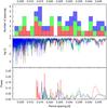 |
Fig. 11 Searching for characteristic period spacings. Notations of the different period sets are the same as in Fig. 9. |
Using Eqs. (1) and (3), we performed similar tests on the periods as on the frequencies in Sect. 5.2.2. Only the histograms and the Fourier transforms suggest the presence of some characteristic spacings around 0.012–0.017, 0.002, 0.024–0.026, and 0.032–0.035 d (cf. Fig. 11). We cannot use and interpret these indefinite results. Modelling of KIC 9533489 might help to decide whether any of these spacing values indeed characterise ℓ modes of the star.
We note that period spacings are strongly influenced not only by chemical gradients, but also by the stellar rotation, especially in the case of moderate and fast rotators, as demonstrated by the theoretical study of Bouabid et al. (2013).
5.2.4. Other regularities
Coupling between g- and p-modes was reported in many hybrids. For CoRoT 105733033 (Chapellier et al. 2012), CoRoT 100866999 (Chapellier & Mathias 2013), and KIC 11145123 (Kurtz et al. 2014), frequencies can be detected in the p-mode regime according to the relation fi,p = F ± fi,g, where fi,g is a g-mode frequency and F is the dominant p-mode: the radial fundamental or a low-overtone frequency. The detection of such a coupling supports the idea that the frequencies found in the low- and high-frequency region originate from the same pulsator. We note that KIC 11145123 is a remarkable textbook example showing how the regular spacings and their deviations can be used to study the stellar interior. Another example of mode coupling is KIC 8054146 (Breger et al. 2012), where peaks were detected in the high-frequency region at f0 + nf1, where f0 is a constant and f1 is the dominant frequency in the low-frequency regime.
We searched for these regularities in the frequency spectrum of KIC 9533489, but only one frequency in the p-mode regime can be explained as the combination of another high-frequency peak and a g-mode frequency, as f50 = f34 + f7 (cf. Table 4), where f50 = 34.14, f34 = 1.56 and f7 = 32.58 d-1. It is worth noting that f34 corresponds to the frequency separation of a triplet, as discussed in Sect. 5.2.2.
6. Transit events
The light curve of KIC 9533489 shows transits, which are shallow (0.5%), short (0.07 d), and recur every 197 days (it is also planetary candidate KOI-3783.01).
First, we checked the field of KIC 9533489 searching for possible external sources that might be responsible for the observed transit events. There are indeed two known stars offset by ~4 and 8 arcsec that are blended within the Kepler photometric aperture. However, these are both too faint to cause eclipses 0.5 per cent deep even if fully eclipsed. Additionally, the Kepler data centroid analysis for this 40σ transit event (averaged over all events) shows that the transit host is coincident with the target star within the 3σ limit of 0.25″. Considering the adaptive optics observation (see Sect. 4), we know that there is an additional star ≈1″ from the primary object. However, it appears to be too faint to be the transit host star, and it is also still too far away from the primary.
We modelled the Kepler LC and SC data using the jktebop code (see Southworth 2008 and references therein), and accounted for the low sampling rate of the LC data by numerically integrating the model to match. Whilst the SC data cover only one transit, their better sampling rate makes them more valuable than the LC data, which cover six transits. We pre-whitened the data to remove the effects of the pulsations, then extracted the regions around each transit and normalised them to unit flux by fitting a straight line to the out-of-transit data.
The transits are indicative of a planetary-mass object orbiting the F0 star, but we encountered problems with this hypothesis. The duration is far too short for this scenario and implies a much smaller radius for the F0 star than found from our spectroscopic analysis. The low ratio of the radii implied by the transit depth also yields transit light curves with ingress and egress durations too short to match the data. These problems forced us to consider the possibility that the putative planet is orbiting a fainter star that is spatially coincident with the F0 star. This allows the use of a higher ratio of the radii, yielding a better match to the durations of the partial phases of the transit, and also implies a smaller stellar radius and thus a shorter transit (Fig. 12).
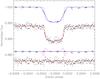 |
Fig. 12 Kepler LC (above) and SC (below) light curves compared to the best fits from jktebop neglecting third light. The residuals are plotted at the base of the figure, offset from unity. The blue and the purple lines through the LC data show the best-fitting model with and without numerical integration, and the ones through the residuals show the difference between this model with and without numerical integration. |
Fitted models of the light curve including a larger “third light” (L3) component are indeed significantly better than those with L3 = 0 (see Fig. 13). Southworth (2012) showed that L3 is very poorly constrained when modelling transits in isolation, but only considered values between 0.0 and 0.75 (expressed as a fraction of the total light of the system). We find that L3 = 0.88 ± 0.03 yields a determinate and improved fit to the light curve. The fainter star should therefore be roughly eight times fainter than the F0 star, which implies a mass of about 0.95 M⊙ if the two stars are at the same distance. We used the DSEP theoretical stellar evolutionary models (Dotter et al. 2008) to guide these inferences of the physical properties of the system.
Whilst a 0.95 M⊙ star has a much smaller radius than the F0 star, we still require a high orbital eccentricity for the transit model to match the observations: esinω = 0.956, where e is orbital eccentricity and ω is the argument of periastron. The high L3 value we find means that a higher ratio of the radii (k = 0.185 versus 0.064) is needed to match the transit depth. Such an object orbiting a 0.95 M⊙ main-sequence star will have a radius of approximately 0.16 R⊙ (1.6 RJup). This is consistent with the radius of an inflated transiting planet (see Southworth et al. 2012), but also with that of a low-mass star. We therefore cannot claim that the transiting object is a planet.
If we allow the transit host star to be closer to Earth than the F0 star, making them merely an asterism instead of gravitationally bound, then its contribution to the system light can be matched by a less massive and thus smaller star. This would mean that the light curve could be matched using a smaller esinω, and also imply a lower radius for the transiting object. We do not currently have sufficient observational constraints to constrain the relative distances of the two stars. Table 6 gives a set of plausible physical properties of the system based on the transit light curves, the DSEP theoretical stellar models, the assumption that the F0 star and the transit host star have a common distance, and that the transiting body is stellar and not an inflated exoplanet.
Plausible model of the KIC 9533489 system.
7. Conclusions
KIC 9533489 is one of the many A–F spectral type stars observed by Kepler. It was selected as a hybrid candidate pulsator by Uytterhoeven et al. (2011). Its hybrid nature, which is most probably genuine, makes it a promising target for detailed analysis. In addition, it shows periodic transit-like events in its light curve.
One of the relevant questions is whether or not KIC 9533489 is a genuine hybrid showing simultaneously self-excited p- and g-modes. The asteroseismic relevance of such genuine hybrids is very high because their structure can be probed down to the deep interior layers. Based on the spectroscopically derived physical parameters of KIC 9533489 showing its location within the overlapping region of the δ Sct and γ Dor instability strips, on the dominant modes’ coupled amplitude variation, and on the strong multiperiodicity in the low frequency domain, we argue that KIC 9533489 is a genuine hybrid pulsator. Furthermore, based on frequency spacing investigations, we conclude that KIC 9533489 is either a highly inclined moderate rotator (v ≈ 70 km s-1, i> 70°) or a fast rotator with v ≈ 200 km s-1 and i ≈ 20°. We need a comprehensive modelling of the star which, among other parameters, takes into account the effects of rotation.
The transit analysis revealed that KIC 9533489 (or the KIC 9533489 system) is unusual. It seems that we have to consider the possibility of a high-order system: the Kepler aperture contains (1) an F0 star showing pulsations; (2) a fainter star at 1″ (detected by the adaptive optics measurements); (3) an (unseen) G/K-type star in the AO PSF of the F0 star (either gravitationally bound or unbound); and (4) a small or faint object transiting the G/K star. Since stellar binaries (or higher order systems) are common, it is certainly possible to have a hierarchical triple system (objects 1, 3, and 4). Further radial velocity observations on a long (years) time-scale and higher signal-to-noise ratio spectra might help to define the spectral type of the unseen transit host star and thus help to characterise the transiting object as well.
IRAF is distributed by the National Optical Astronomy Observatories, which are operated by the Association of Universities for Research in Astronomy, Inc., under cooperative agreement with the National Science Foundation.
Acknowledgments
The authors thank the anonymous referee for the constructive comments and recommendations on the manuscript. Zs.B. acknowledges the support of the Hungarian Eötvös Fellowship (2013), the kind hospitality of the Royal Observatory of Belgium as a temporary voluntary researcher (2013–2014), and, together with Á.S., the support of the ESA PECS project 4000103541/11/NL/KML. Á.S. acknowledges support by the Belgian Federal Science Policy (project M0/33/029, PI: P.D.C.) and by the János Bolyai Research Scholarship of the Hungarian Academy of Sciences. P.M.F. acknowledges support from MICINN of Spain via grants BES-2012-053246 and AYA2011-24728, and from the “Junta de Andalucía” through the FQM-108 project. Funding for the Kepler mission is provided by the NASA Science Mission directorate. We thank the Kepler team for the high-quality data obtained by this outstanding mission. We are very grateful to Jorge Jiménez Vicente (Universidad de Granada, Spain) and Evencio Mediavilla (Instituto de Astrofísica de Canarias) for kindly providing a spectrum with the INTEGRAL optical fiber system. Based on spectra obtained with the HERMES spectrograph installed at the Mercator Telescope, operated by the Flemish Community, with the Nordic Optical Telescope, operated by the Nordic Optical Telescope Scientific Association, and with the William Herschel Telescope, operated by the Isaac Newton Group of Telescopes. All instruments are located at the Observatorio del Roque de los Muchachos, La Palma, Spain, of the Instituto de Astrofisica de Canarias. Some of the data presented herein were obtained at the W. M. Keck Observatory, which is operated as a scientific partnership among the California Institute of Technology, the University of California and the National Aeronautics and Space Administration. The Observatory was made possible by the generous financial support of the W. M. Keck Foundation. The authors thank Simon Murphy for his useful comments on the first version of this manuscript.
References
- Aerts, C., Christensen-Dalsgaard, J., & Kurtz, D. W. 2010, Asteroseismology (Springer Science+Business Media B.V.), Astronomy and Astrophsyics Library [Google Scholar]
- Arribas, S., Carter, D., Cavaller, L., et al. 1998, in Optical Astronomical Instrumentation, ed. S. D’Odorico, SPIE Conf. Ser., 3355, 821 [NASA ADS] [CrossRef] [Google Scholar]
- Auvergne, M., Bodin, P., Boisnard, L., et al. 2009, A&A, 506, 411 [NASA ADS] [CrossRef] [EDP Sciences] [Google Scholar]
- Balona, L. A. 2011, MNRAS, 415, 1691 [NASA ADS] [CrossRef] [Google Scholar]
- Balona, L. A. 2014, MNRAS, 437, 1476 [NASA ADS] [CrossRef] [Google Scholar]
- Bouabid, M.-P., Montalbán, J., Miglio, A., et al. 2011, A&A, 531, A145 [NASA ADS] [CrossRef] [EDP Sciences] [Google Scholar]
- Bouabid, M.-P., Dupret, M.-A., Salmon, S., et al. 2013, MNRAS, 429, 2500 [NASA ADS] [CrossRef] [Google Scholar]
- Breger, M. 2000, in Delta Scuti and Related Stars, eds. M. Breger, & M. Montgomery, ASP Conf. Ser., 210, 3 [Google Scholar]
- Breger, M., Stich, J., Garrido, R., et al. 1993, A&A, 271, 482 [NASA ADS] [Google Scholar]
- Breger, M., Fossati, L., Balona, L., et al. 2012, ApJ, 759, 62 [NASA ADS] [CrossRef] [Google Scholar]
- Castelli, F., & Kurucz, R. L. 2004, ArXiv e-prints [arXiv:astro-ph/0405087] [Google Scholar]
- Chapellier, E., & Mathias, P. 2013, A&A, 556, A87 [NASA ADS] [CrossRef] [EDP Sciences] [Google Scholar]
- Chapellier, E., Mathias, P., Weiss, W. W., Le Contel, D., & Debosscher, J. 2012, A&A, 540, A117 [NASA ADS] [CrossRef] [EDP Sciences] [Google Scholar]
- Chlebowski, T. 1978, Acta Astron., 28, 441 [NASA ADS] [Google Scholar]
- Dotter, A., Chaboyer, B., Jevremović, D., et al. 2008, ApJS, 178, 89 [NASA ADS] [CrossRef] [Google Scholar]
- Dupret, M.-A., Grigahcène, A., Garrido, R., Gabriel, M., & Scuflaire, R. 2004, A&A, 414, L17 [NASA ADS] [CrossRef] [EDP Sciences] [Google Scholar]
- Dziembowski, W. A., & Goode, P. R. 1992, ApJ, 394, 670 [NASA ADS] [CrossRef] [Google Scholar]
- Frémat, Y., Lampens, P., van Cauteren, P., et al. 2007, A&A, 471, 675 [NASA ADS] [CrossRef] [EDP Sciences] [Google Scholar]
- García Hernández, A., Moya, A., Michel, E., et al. 2009, A&A, 506, 79 [NASA ADS] [CrossRef] [EDP Sciences] [Google Scholar]
- Gilliland, R. L., Jenkins, J. M., Borucki, W. J., et al. 2010, ApJ, 713, L160 [NASA ADS] [CrossRef] [Google Scholar]
- Girardi, L., Bressan, A., Bertelli, G., & Chiosi, C. 2000, A&AS, 141, 371 [NASA ADS] [CrossRef] [EDP Sciences] [Google Scholar]
- Gough, D. O. 1990, in Progress of Seismology of the Sun and Stars, eds. Y. Osaki, & H. Shibahashi, Lecture Notes in Physics (Berlin: Springer Verlag), 367, 283 [Google Scholar]
- Gough, D. O., & Thompson, M. J. 1990, MNRAS, 242, 25 [NASA ADS] [CrossRef] [Google Scholar]
- Gray, D. F. 1992, The observation and analysis of stellar photospheres (Cambridge University Press) [Google Scholar]
- Grigahcène, A., Antoci, V., Balona, L., et al. 2010, ApJ, 713, L192 [NASA ADS] [CrossRef] [Google Scholar]
- Guzik, J. A., Kaye, A. B., Bradley, P. A., Cox, A. N., & Neuforge, C. 2000, ApJ, 542, L57 [NASA ADS] [CrossRef] [Google Scholar]
- Handler, G., Pikall, H., O’Donoghue, D., et al. 1997, MNRAS, 286, 303 [NASA ADS] [CrossRef] [Google Scholar]
- Handler, G., Balona, L. A., Shobbrook, R. R., et al. 2002, MNRAS, 333, 262 [NASA ADS] [CrossRef] [Google Scholar]
- Hareter, M. 2012, Astron. Nachr., 333, 1048 [NASA ADS] [Google Scholar]
- Henry, G. W., & Fekel, F. C. 2005, AJ, 129, 2026 [NASA ADS] [CrossRef] [Google Scholar]
- Howell, S. B., Rowe, J. F., Bryson, S. T., et al. 2012, ApJ, 746, 123 [NASA ADS] [CrossRef] [Google Scholar]
- Hubeny, I., & Lanz, T. 1995, ApJ, 439, 875 [Google Scholar]
- Jenkins, J. M., Caldwell, D. A., Chandrasekaran, H., et al. 2010, ApJ, 713, L120 [NASA ADS] [CrossRef] [Google Scholar]
- Kawaler, S. D. 1988, in Advances in Helio- and Asteroseismology, eds. J. Christensen-Dalsgaard, & S. Frandsen, IAU Symp., 123, 329 [Google Scholar]
- Kjeldsen, H., Arentoft, T., Bedding, T., et al. 1998, in Structure and Dynamics of the Interior of the Sun and Sun-like Stars, ed. S. Korzennik, ESA SP, 418, 385 [NASA ADS] [Google Scholar]
- Koch, D. G., Borucki, W. J., Basri, G., et al. 2010, ApJ, 713, L79 [NASA ADS] [CrossRef] [Google Scholar]
- Kurtz, D. W., Saio, H., Takata, M., et al. 2014, MNRAS, 444, 102 [NASA ADS] [CrossRef] [Google Scholar]
- Lampens, P., Tkachenko, A., Lehmann, H., et al. 2013, A&A, 549, A104 [NASA ADS] [CrossRef] [EDP Sciences] [Google Scholar]
- Lenz, P., & Breger, M. 2005, Commun. Asteroseismol., 146, 53 [NASA ADS] [CrossRef] [Google Scholar]
- Matthews, J. M. 2007, Commun. Asteroseismol., 150, 333 [NASA ADS] [CrossRef] [Google Scholar]
- Miglio, A., Montalbán, J., Noels, A., & Eggenberger, P. 2008, MNRAS, 386, 1487 [NASA ADS] [CrossRef] [Google Scholar]
- Murphy, S. J. 2012, MNRAS, 422, 665 [NASA ADS] [CrossRef] [Google Scholar]
- Murphy, S. J., Shibahashi, H., & Kurtz, D. W. 2013, MNRAS, 430, 2986 [NASA ADS] [CrossRef] [Google Scholar]
- Murphy, S. J., Bedding, T. R., Shibahashi, H., Kurtz, D. W., & Kjeldsen, H. 2014, MNRAS, 441, 2515 [Google Scholar]
- Paparó, M., Bognár, Z., Benkő, J. M., et al. 2013, A&A, 557, A27 [NASA ADS] [CrossRef] [EDP Sciences] [Google Scholar]
- Pápics, P. I. 2012, Astron. Nachr., 333, 1053 [NASA ADS] [CrossRef] [Google Scholar]
- Raskin, G., van Winckel, H., Hensberge, H., et al. 2011, A&A, 526, A69 [NASA ADS] [CrossRef] [EDP Sciences] [Google Scholar]
- Reegen, P. 2007, A&A, 467, 1353 [NASA ADS] [CrossRef] [EDP Sciences] [Google Scholar]
- Royer, F. 2005, Mem. Soc. Astron. It. Suppl., 8, 124 [Google Scholar]
- Southworth, J. 2008, MNRAS, 386, 1644 [NASA ADS] [CrossRef] [Google Scholar]
- Southworth, J. 2012, MNRAS, 426, 1291 [NASA ADS] [CrossRef] [Google Scholar]
- Southworth, J., Hinse, T. C., Dominik, M., et al. 2012, MNRAS, 426, 1338 [NASA ADS] [CrossRef] [Google Scholar]
- Stellingwerf, R. F. 1979, ApJ, 227, 935 [NASA ADS] [CrossRef] [Google Scholar]
- Stoehr, F., Fraquelli, D., Kamp, I., et al. 2007, Space Telescope European Coordinating Facility Newsletter, 42, 4 [NASA ADS] [Google Scholar]
- Suárez, J. C., García Hernández, A., Moya, A., et al. 2014, A&A, 563, A7 [NASA ADS] [CrossRef] [EDP Sciences] [Google Scholar]
- Tassoul, M. 1980, ApJS, 43, 469 [NASA ADS] [CrossRef] [Google Scholar]
- Unno, W., Osaki, Y., Ando, H., Saio, H., & Shibahashi, H. 1989, Nonradial oscillations of stars (Tokyo: University of Tokyo Press), 2nd edn. [Google Scholar]
- Uytterhoeven, K., Moya, A., Grigahcène, A., et al. 2011, A&A, 534, A125 [NASA ADS] [CrossRef] [EDP Sciences] [Google Scholar]
- Vogt, S. S., Allen, S. L., Bigelow, B. C., et al. 1994, in Instrumentation in Astronomy VIII, eds. D. L. Crawford, & E. R. Craine, SPIE Conf. Ser., 2198, 362 [Google Scholar]
- Walker, G., Matthews, J., Kuschnig, R., et al. 2003, PASP, 115, 1023 [NASA ADS] [CrossRef] [Google Scholar]
- Willems, B., & Aerts, C. 2002, A&A, 384, 441 [NASA ADS] [CrossRef] [EDP Sciences] [Google Scholar]
- Zima, W. 2008, Commun. Asteroseismol., 155, 17 [Google Scholar]
All Tables
Effective temperature values derived from the fit of the hydrogen line profiles observed with different instruments.
Stellar parameters of KIC 9533489, determined from spectroscopic observations (“spectra”) and evolutionary tracks and isochrones (“models”, Girardi et al. 2000).
Possible rotational periods (P), equatorial velocities (v), and inclinations (i) of KIC 9533489 derived by applying different frequency spacing values.
All Figures
|
Fig. 1 Observed HIRES spectrum (in black) and synthetic model (in red) of an F0-type star with v sin i = 70 km s-1 over the wavelength range 400–455 nm. The residual spectrum is drawn in blue. |
| In the text | |
|
Fig. 2 Location of KIC 9533489 on the surface gravity vs. effective temperature diagram. Evolutionary tracks for 1.4, 1.5, 1.6, and 1.7 M⊙, as derived by Girardi et al. (2000) are plotted with solid lines. Dotted lines show 63 Myr –1.12 Gyr isochrones. |
| In the text | |
|
Fig. 3 Keck II adaptive optics image of KIC 9533489. |
| In the text | |
|
Fig. 4 Fourier transforms of the original SC light curve and of the light curve pre-whitened for 2, 9, 46, and 63 frequencies. The blue dashed lines denote the 4 ⟨ A ⟩ significance level, where ⟨ A ⟩ is calculated as the moving average of radius 8 d-1 of the pre-whitened spectrum. The frequency gap between ≈15 and 27 d-1 is indicated with a grey band. The vertical dotted line denotes the Nyquist limit of the LC data. |
| In the text | |
|
Fig. 5 Fourier transforms of the original SC (upper panel) and LC (bottom panel) light curve. The frequency gap between ≈15 and 27 d-1 found in the SC data is indicated with a grey band. The vertical dotted line denotes the Nyquist limit of the LC data. Red lines connect the lowest and highest frequency peaks of the SC data with their Nyquist aliases detected in the LC Fourier transform. |
| In the text | |
|
Fig. 6 Section of the SC light curve of KIC 9533489 and the fit of the two dominant frequencies (red line). The plot exhibits the beating effect that dominates the light variations. |
| In the text | |
|
Fig. 7 Amplitudes of f1 and f2 in the different light-curve segments of the Q1–Q17 LC data. The dashed line shows the error-weighted average of the data points, the continuous line is a linear fit to the data. |
| In the text | |
|
Fig. 8 Time delays calculated for the two dominant modes f1 and f2 (top panels), and their Fourier transform (bottom panels). |
| In the text | |
|
Fig. 9 Searching for characteristic frequency spacings. From top to bottom: histograms of frequency differences, results of K-S tests, Fourier transforms of different frequency sets. Red boxes/lines: frequencies below 5 d-1, green boxes/lines: frequencies below 10 d-1, blue boxes/lines: frequencies below 15 d-1, grey boxes/lines: frequencies above 27 d-1. |
| In the text | |
|
Fig. 10 Echelle diagrams of the 12 independent frequencies, supposed p-modes, above the frequency gap. |
| In the text | |
|
Fig. 11 Searching for characteristic period spacings. Notations of the different period sets are the same as in Fig. 9. |
| In the text | |
|
Fig. 12 Kepler LC (above) and SC (below) light curves compared to the best fits from jktebop neglecting third light. The residuals are plotted at the base of the figure, offset from unity. The blue and the purple lines through the LC data show the best-fitting model with and without numerical integration, and the ones through the residuals show the difference between this model with and without numerical integration. |
| In the text | |
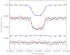 |
Fig. 13 As Fig. 12 but allowing for third light when calculating the best fit. |
| In the text | |
Current usage metrics show cumulative count of Article Views (full-text article views including HTML views, PDF and ePub downloads, according to the available data) and Abstracts Views on Vision4Press platform.
Data correspond to usage on the plateform after 2015. The current usage metrics is available 48-96 hours after online publication and is updated daily on week days.
Initial download of the metrics may take a while.