| Issue |
A&A
Volume 581, September 2015
|
|
|---|---|---|
| Article Number | A134 | |
| Number of page(s) | 79 | |
| Section | Catalogs and data | |
| DOI | https://doi.org/10.1051/0004-6361/201525810 | |
| Published online | 22 September 2015 | |
High spectral resolution monitoring of Nova V339 Delphini with TIGRE
1 Hamburger Sternwarte, Universität Hamburg, Gojenbergsweg 112, 21029 Hamburg, Germany
e-mail: This email address is being protected from spambots. You need JavaScript enabled to view it.
2 Departamento de Astronomía, Universidad de Guanajuato, Apartado Postal 144, 36000 Guanajuato, Mexico
3 Department of Astrophysics, Geophysics and Oceanography, University of Liège, 17 allée du 6 Août, B5c, 4000 Sart Tilman, Belgium
Received: 5 February 2015
Accepted: 7 July 2015
Abstract
Aims. We investigate the early development of the classical nova V339 Del (Nova Delphini 2013) through high-resolution optical spectroscopy. To study the structure of the ejecta, we focus on the evolution of the absorption and emission features and the changes within the line profiles.
Methods. We obtained spectra with the robotic 1.2 m telescope TIGRE equipped with the HEROS spectrograph (R = 20 000, wavelength coverage from 3800 to 8800 Å). Our data set covers the outburst from 3 until 121 days after discovery.
Results. We provide a qualitative analysis of the spectra, describing the line profiles evolution and providing a rich list of identified lines. During the optically thick phase, we detected several blue-shifted absorption features from s-processed elements, whose origin is unclear. The presence of strong lines from C/O and the absence of Neon features confirm that the nature of the central white dwarf is a CO type. The later “nebular” phase spectra show evidence of the non-spherical, inhomogeneous structure of the ejecta. The detailed evolution of the line profiles and appearance of high ionization species (e.g. N III, O III, He II, [Fe VII]) are direct consequences of the re-ionization of the ejecta during the peak of the soft X-ray emission.
Key words: novae, cataclysmic variables / stars: individual: V339 Del / stars: emission-line, Be / instrumentation: spectrographs / telescopes
© ESO, 2015
1. Introduction
Classical novae are thought to be explosive mass ejections triggered by a thermonuclear runaway on the surface of a white dwarf accreting mass from a Roche-lobe-filling companion. Novae eruptions are a spectacular phenomenon that has been extensively studied since the first half of the 20th century, with Payne-Gaposchkin (1964) still offering a formidable review of the topic. While classical novae as such are relatively common, naked-eye visible novae are quite rare, typically occurring every other decade, and γ-ray emitting novae represent quite extraordinary events. Reaching an estimated maximum brightness of V = 4.46 mag on August 16.4 UT (Munari et al. 2013), the nova V339 Del (Nova Delphini 2013, PNV J20233073+2046041) did provide the rare chance of a really bright nova, which in addition was detected as a γ-ray source with Fermi-LAT four days after its eruption (Hays et al. 2013).
A solid picture and understanding of the nova phenomenon could be built from a variety of multi-wavelength campaigns conducted in the past two decades, followed by theoretical advancements of the field (see Bode & Evans 2008 for recent reviews), and yet the first detection of high energy γ-ray emission (>100 MeV) from a classical nova (Cheung et al. 2012) came unexpectedly and still lacks a definite explanation.
The unusual brightness of V339 Del made it the subject of intensive multi-wavelength monitoring in various wavelengths: γ-rays: Ackermann et al. (2014); X-rays: Page & Beardmore (2013); optical: Skopal et al. (2014), Tajitsu et al. (2015); near-IR: Schaefer et al. (2014). In archival data Deacon et al. (2014) were able to identify its progenitor as an object of magnitude V ~ 17 mag without any significant photometric variability, at least in the last years. With our TIGRE robotic spectroscopic telescopes, we performed high spectral resolution monitoring in the optical covering the first four months of the outburst.
TIGRE spectra.
2. Observations and data reduction
We present our spectroscopic observations of V339 Del with the robotic TIGRE 1.2 m telescope, located near Guanajuato in central Mexico and equipped with the HEROS spectrograph. It provides a spectral resolution of 20 000 over the visual spectral range from 3800 to 8800 Å with a small gap (between the two arms) from 5700 to 5830 Å. The TIGRE spectra are reduced with the standard spectral reduction pipeline for TIGRE/HEROS. The spectra are not flux-calibrated. This prevents us from estimating the brightness or from using emission lines fluxes diagnostics, which usually rely on emission-line strength ratios. Nevertheless, the high resolution and wide spectral range allowed us to correctly identify many absorption and emission features and to resolve the fine structures in the line profiles in order to study the kinematics of the ejecta.
For a technical description of TIGRE and its instrumentation, see Schmitt et al. (2014). The concise science and operation management of this TIGRE, funded by the Universities of Hamburg, Guanajuato, and Liège, and its flexible scheduling allowed us to start observations on day +3 after discovery, close to maximum light in the V band, and to follow it until four months later.
In Table 1 we list the nights during which we were able to obtain spectra of V339 Del. Hereafter, we refer to the different observing nights of the nova with the number of days passed since its discovery by K. Itagaki on 2013-08-14.584 (CBET 3628). The V-mag values were extracted using the AAVSO lightcurve generator and are shown in Fig. 1, where we also indicate the times for which TIGRE spectra are available.
The result of these observations is a spectral atlas that documents the line profiles and the line content of the different stages of the nova evolution from the optically thick phase, as observed during the early nights, until the optically thin nebula phase of the then much expanded nova envelope. The spectra presented here allow us a rich and certain line identification, a documentation of the changing line content, and profile shapes, including rather unusual transitions in novae spectra and some signatures of non-spherical ejecta geometry or inhomogeneity. In these terms, high-resolution spectroscopy of novae is indeed necessary for investigating their evolutionary details and physical processes. We here attempt a phenomenological overview of the achieved spectroscopic monitoring of V339 Del.
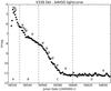 |
Fig. 1 Lightcurve of V339 Del in the V band. The dots represent daily averages from the AAVSO data. The vertical lines separate the different phases discussed in Sect. 3: A. optically thick; B. transition; C. early nebular; D. late nebular. The triangles mark the TIGRE observations (Table 1). |
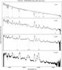 |
Fig. 2a TIGRE/HEROS spectra from days +3 (optically thick phase), +15 (transition phase), +42 (early nebular phase), and +121 (late nebular phase) after discovery. Blue channel. The spectra are blaze-normalized and subsequently normalized to a polynomial instrumental response function. No absolute flux calibration has been applied. Flux is shown on a logarithmic scale to better display the several spectroscopic features. The most relevant lines are numbered in italics, and for their identifications see Table 2. |
3. The line spectrum of V339 Del: Overview
We organize our description of the TIGRE spectra in terms of the characteristic stages of the nova development. Our observations on nights +3, +5, and +6 cover the optically thick phase of the young and compact nova shell, showing prominent P-Cygni-type line profiles from lowly ionized species. On day +15, an emission line spectrum has emerged, but with the first forbidden lines appearing and many strong lines still showing a residual P-Cyg absorption, so we are clearly witnessing a transition phase. From day +42 on, the nova ejecta show a pure emission line spectrum, with most of the emerging flux concentrated in individual lines. The last observation on day +121 lets us witness the spectral response of the ejecta to the X-ray turn-on of the white dwarf, which re-ionizes the gas. We show a selection of the recorded TIGRE spectra, taking one spectrum from each of the characteristic phases outlined above for the blue channel in Fig. 2a and for the red channel in Fig. 2b. Figure 3 provides an evolution graph of the ionization potentials for the ionized species identified in our spectra.
A rather large collection of amateur spectra of V339 Del has been collected and made publicly available by the members of the Astronomical Ring for Access to Spectroscopy (ARAS) project1. This data set covers a large time span from approximately five hours after discovery until ~600 days after discovery, with spectral resolution ranging from 500 to 10 000. These observations have been discussed in Shore et al. (2013f,a,b) and Skopal et al. (2014).
There has been some controversy over the detailed line content of V339 Del, as seen in Skopal et al. (2014) and Shore et al. (2014). Obviously, high spectral resolution helps enormously to narrow down the range of hypothetical line matches. The finding list provided by Williams (2012) was used to determine the transitions, but its accuracy of only 1 Å was insufficient to reliably identify many of the lines in our spectra, therefore we also made extensive use of the NIST database (Kramida et al. 2014) for more precise wavelength values. Moreover, the identification of transient heavy elements reported in Williams et al. (2008) greatly helped us to properly recognize many of the narrow absorption features. We report the identified lines list at the end of Sect. 4.
For the line profiles radial velocity plots in Sect. 4, we have adopted the heliocentric velocity frame.
4. Spectral evolution: P-Cygni to pure emission lines
4.1. Optically thick phase
The first three spectra obtained with TIGRE (on +3, +5, and +6 days after discovery) show a large number of absorption features typical of the optically thick phase (Fig. 2, 1st panel; Fig. 4). Several species (H I, C I, Ca II, Fe II, O I) exhibit clear P-Cyg profiles. Moreover, a multitude of lowly ionized species, i.e. Cr II, Fe I, Mg II, Na I, Sc II, Si II, Sr II, Ti II, show only narrow absorption features with radial velocities covering a narrow range in radial velocity between −500 and −800 km s-1 (Fig. 5).
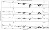 |
Fig. 2b continued − Red channel. |
The H I transitions are strong and well resolved. On day +3 their P-Cyg profiles show a smooth absorption with terminal velocity up to −2000 km s-1. The appearance of these profiles, i.e., the depth and width of the absorption and the strength of the emission peak, are naturally different for each transition. Already on day +5, we see such differences; for example, Hα (Fig. 6) features a rather smooth profile (contaminated by telluric lines, which have not been removed from these spectra), while the other H I lines show fragmented P-Cyg absorption troughs. This is typical behaviour for novae, which hints at the filamentous and inhomogeneous structure of the ejected gas (Shore et al. 2011).
The multitude of Fe I–II lines clearly show the ongoing line blanketing by an “Fe II curtain”: because of the low temperature in the ejecta of the order of 104 K or lower, several metallic species are only lowly ionized and therefore dominate the optical depth of the expanding envelope and thus redistribute the radiative energy from the UV into the optical wavelength range (see Hauschildt et al. 1997).
The narrow absorption features observed for the lowly ionized species are characterized by a small velocity dispersion, between −500 and −800 km s-1 as aforementioned. The group of Williams et al. conducted an extensive observational campaign on classical and recurrent novae and systematically observed these features from s-process elements for several days or weeks (Williams et al. 2008; Mason 2011). In our set of TIGRE spectra, we only observed such features from day +3 to +6. The absence of an emission counterpart on the red side of these lines is due to the transitions being optically thick in the visible band, which favours the appearance of only an absorption feature, since it mainly depends on the column density. For the same reason, highly ionized species are not observed in this phase because they are optically thick throughout the visible band.
While many of these species are only observed on day +3, the strongest Fe II transitions remain clear throughout the early development and show the typical bluewards displacement commonly observed in high-resolution studies (Fig. 7). This phenomenon was explained by Shore et al. (2011) and stems from the combined effect of steady expansion and cooling: the inner, slower gas recombines faster because of higher density, with a recombination front progressing outwards and tracing the faster moving, but thinner outer gas.
In addition, there are tiny, not clearly resolved or weak absorption features that are difficult to identify, but they likely originate in lowly ionized metals as well.
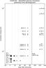 |
Fig. 3 Ionized species observed throughout the observational campaign. The dotted vertical lines indicate the different phases introduced in Sect. 3. The full vertical line corresponds to the peak of the soft X-ray emission (details in Sect. 4). |
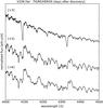 |
Fig. 4 On day +3, the two most relevant lines seen here are Hγ and Hδ, both exhibiting P-Cyg-like profiles, while the other species, mainly Fe II, show only narrow absorption features. Later (days +5 and +6) the spectrum consists of a multitude of wide, overlapping emission line profiles. |
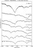 |
Fig. 5 Low ionization stages of heavy elements identified during the optically thick phase (day +3 in this case), with Hζ as a reference. The dotted vertical line marks −660 km s-1 on the radial velocity scale used here. |
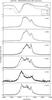 |
Fig. 6 Hα and Hβ development through the whole time span. |
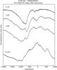 |
Fig. 7 Development of Fe II 4923.3 Å in the early phase, showing the progression of the minimum of the absorption towards higher negative velocities. The vertical dotted line marks a radial velocity of −660 km s-1, as in Fig. 5. |
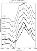 |
Fig. 8 Hδ development during the transition phase. The spectra are normalized to the peak of the line and vertically shifted. |
4.2. Transition phase
The TIGRE observations from day +15 (Fig. 2, 2nd panel) show the evolution of the ejecta during the lifting of the “Fe-II curtain”. This process is driven by the envelope’s expansion, which steadily rarefies the gas and by the hot radiation field from the central white dwarf, which is about to turn into a super-soft X-ray source (see below). The spectrum now looks “hotter”, with strong H I lines showing a weak P-Cyg absorption (which is stronger for the lines higher up in the Balmer series) and strong central emission. Each line is now evidently showing a non-sphericity of the ejecta, with a clear peak present at +600 km s-1 in many line profiles.
The asymmetry of the line profiles at this stage, with the red side brighter than the blue side, is caused by the still high optical depth of the gas. At the same time, the appearance of forbidden lines from [N I] and [O I] marks the transition towards the “nebular”, optically thin phase of the nova shell. The appearance of the lines in this phase remains approximately constant. Hα (Fig. 6) no longer exhibits a true P-Cyg profile, but rather a heavily dimmed blue side. For the other H I lines, the line profiles from days +15 to +28 show a P-Cyg absorption that undergoes only subtle development (e.g., Hδ development in Fig. 8). The absorption spans a velocity range from −700 to −1350 km s-1, but it is clearly made of a number of small features evolving over time as optical depth steadily decreases during the expansion. For other species showing P-Cyg profile in the transition phase, we observe the same velocity range for Ca II K, but lower terminal velocities, approximately −1200 km s-1, for the strongest Fe II transitions, i.e., λ 4233, 5016, 5168 Å, which is again only an optical depth effect since the differences in the profile for each species are the result of different ionization and line opacity.
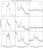 |
Fig. 9 From top to bottom, the nebular phase development for Hα 6562 Å, He II 4686,Å and [Fe VII] 6087, showing the re-enhancement of the core of the first two lines and the appearance of the [Fe VII] line. |
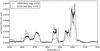 |
Fig. 10 Comparison between V339 Del (day +121) and the ONe nova V959 Mon (day +152), illustrating the absence of [Ne IV] 4714, 4725 Å lines in Nova Del 2013. |
4.3. Optically thin phase
The spectrum taken on day +42, shown in the third panel of Fig. 2 provides evidence that the ejecta are definitely in their “nebular” phase. The density of the ejected gas decreases continuously. If we assume a single ballistic ejection with constant mass and linear velocity law v ~ r, we have ρ ~ t-3. As a result, the density has decreased by three orders of magnitude if we compare this stage with the optically thick phase. Likewise, the column density steadily decreases, as is evident from the disappearance of P-Cyg absorption profiles. The ionization level of the gas increases, as we can see from the appearance of He I lines and [O III] 5007 Å (the lines at 4363 and 4959 Å appear only later, along with N III features and He II 4686 Å, see for example Fig. 2a). Another typical species that indicates the nebular phase is [N II], the strongest transitions of which are at 5755, 6548, 6583Å. Unfortunately, the first line falls exactly into the gap between the two spectral arms of HEROS (but is present in the spectrum, as reported by Shore et al. 2013d), and the other two lines are heavily blended with Hα. Based on our spectra, however, there is no clear evidence of any such blend – compare directly Hα and Hβ profiles (Fig. 6) – in terms of an apparent extra component in radial velocity. In particular, [N II] 6583 Å is an equivalent of ~1000 km s-1 to the red side of Hα, and in all the spectra obtained, there is no evidence of any such contamination at that velocity.
Thanks to wide spectral range of our observations, we can follow the evolution of many species, while the high resolution allows us to look at fine details in the line profiles. For example, from day +42, He I appears to be a remarkably strong emitter represented by several lines, while its transitions are not detectable in the spectrum up to day +28. The Ca II K line, which undergoes a slow fading during the transition phase, is only visible on day +42. The O I and [O I] transitions slowly fade away, and higher ionization stages like [O III] start appearing. These fast changes in the spectral appearance follow the steady expansion of the gas and the evolution of the ionizing radiation field deep inside the ejecta. While the gas density is dropping, the forbidden lines increase in strength, and the radiation from the hot photosphere of the remnant central white dwarf re-ionizes the medium (see below). The lines unaffected by contamination show a wide profile with full-width-zero-intensity of 3000 km s-1. Several lines, however, do show double-peaked emission profiles, such as H I, He I–II, C II, Fe II, O I, and [O I], with a central core half-width of approximately 200 km s-1 and two distinct peaks at roughly +/−700 km s-1, a value corresponding with the radial velocity of the detached absorption features observed during the optically thick phase. The side emission peaks have, however, different fluxes in the blue and red peaks. This is evident for H I and He I–II lines, but also for [O III] lines. Forbidden lines are characterized by very low transition rates, Aij ≲ 10-2 s-1, when compared to permitted lines, i.e. Aij ~ 107 s-1. Therefore, optical depth effects play no role in shaping the line profiles of forbidden lines. We note that the same phenomenon also characterizes the emission lines in the UV spectra (Shore et al. 2013e).
The possibility and evidence of non-spherical nova ejecta have been recently discussed by Shore (2013). Such a scenario may well explain the multiple-component structure of different species in the course of the long optically thin emission phase and their respective time variability, as is evident from Fig. 6, and elsewhere. Therefore the observed behaviour may be explained in terms of a tilted (against the line of sight) bipolar ejecta structure, where the fast material of the growing front lobe starts to intersect the line of sight at some intermediate state of the optically thin phase. An envelope of more excited material around such a lobe would then explain the asynchronous time behaviour of the radial velocity components in the He I–II lines mentioned above. However, random inhomogeneities within the bipolar ejecta may also explain the slight differences between the red and blue sides of the profiles.
4.4. Spectral evidence of the bright X-rays central source
The late spectra of novae require multi-wavelength coverage to fully comprehend these objects. Understanding the X-ray emission is necessary in the initial and later phases (Schwarz et al. 2011). Owing to shocks between dense layers of fast-moving gas, some novae show an early, rapidly declining, hard X-ray emission with typical energies above 1 keV. Later in the expansion of the ejecta, the column density of the gas drops sufficiently to reveal the hot remnant WD. Owing to its high effective temperature, typically 2 − 8 × 10⁵ K, the emission peaks in the soft X-rays, with energies well below 1 keV.
V339 Del was detected as a weak hard X-ray source on day +36 (Page & Beardmore 2013), and the first super-soft X-ray source (SSS) emission was detected on day +63 (Page et al. 2013). It then became a bright SSS (Osborne et al. 2013) and peaked 88 days after discovery (Beardmore et al. 2013). The spectrum obtained on day +121 shows evidence of the strong, ionizing radiation field from the remnant white dwarf. The continuously expanding ejecta were re-ionized by the highly energetic radiation from the central source.A good indicator of this process is the appearance of highly ionized species, the best example being [Fe VII] 6087 Å (shown in Fig. 9). Several other species, such as the Balmer series He I–II, [O III] 5007 Å, show some enhancement of the central core of the profile, hinting at a re-ionization event and a reset of recombination in the denser, slower regions of the ejecta. Since these changes must come with some delay from the establishment of a significant strong X-ray radiation field, the spectral behaviour observed here is fully consistent with the X-ray observations of V339 Del.
An important parameter for determining the ejected mass is the “turn-on” time of the SSS (Schwarz et al. 2011). This could be easily measured with continuous X-ray monitoring of novae, but it requires space-based observatories. At first glance, the appearance of lines from highly ionized species in the optical spectra may help in the task. Super-soft emission can be observed when the column density of the ejecta has decreased to the point where the gas is X-ray transparent. Therefore, it does not necessarily correspond to the appearance of highly ionized species. Even if day +63 is taken as “X-ray turn-on” time, we do not see strongly ionized species on day +72. The appearance of [Fe VI/VII] lines must have occurred between days +72 and +121 during the peak of the SSS emission, a period for which we lack observations. Even higher ionization lines of Fe, mainly [Fe X] 6375 Å, are commonly observed in novae. In V339 Del, however, we do not detect such lines, in agreement with the ARAS forum, who only report the detection of [Fe VII]2.
4.5. CO white dwarf
Shore et al. (2013g) characterize V339 Del as a CO nova. We agree with this identification, given the lack of Ne lines and the multitude and strength of C and O lines in our spectra. A direct comparison with the ONe classical nova V959 Mon (Shore et al. 2013c; Fig. 10) in a similar stage of the outburst supports the absence of the [Ne IV] 4714, 4725 Å lines, which are typical in ONe novae nebular phase. Furthermore, Nelson et al. (2013) and Ness et al. (2013) report strong C absorption features in, respectively, Chandra and XMM-Newton spectra.
4.6. Spectral line atlas
The long-term monitoring with TIGRE allowed us to observe the nova developing from the optically thick stage, with the spectrum rich in P-Cyg lines and narrow absorption features, to the nebular phase, when only emission lines are observed. This puts us in the position to build a spectral line atlas (provided in Table 2), where we included all the spectral lines that we are confident of having identified correctly. For the initial phase of the nova, approximately half of those lines were identified through direct comparison with line profile plots on a radial velocity scale, because many of the nova ejecta lines only show blue-shifted absorption components. This kind of analysis is only possible with high-resolution spectroscopy (R> 10 000) as provided by TIGRE, which allows us to study the development of the line profiles in detail and properly resolve substructure in velocity space.
Table 2 also includes lines that lack a clear identification. They are detected in all the spectra from the optically thick phase as absorption features. As mentioned in Sect. 4.1, they are likely to be due to lowly ionized metallic species. Consequently, the wavelength values provided in Table 2 are such that the radial velocity of these features corresponds to −660 km s-1, the same value as was adopted for Fig. 5.
The complete collection of profiles, showing the full development of each identified line, is available as on-line material.
5. Summary and conclusions
We have presented a time sequence of high-resolution (R = 20 000) spectra, obtained by the 1.2 m robotic TIGRE telescope and its HEROS spectrograph, monitoring Nova Delphini 2013 from day 3 to day 121 after its discovery.
The broad spectral coverage (almost the whole spectrum between 3800 and 8800 Å with only a small gap) allows us to clearly resolve, identify, and monitor the behaviour of over a hundred different lines, which are produced by ions of many different excitation and ionization energies. Certainly, there is evidence of many more lines, most of which are either weak, blended, or both. As a result, the spectral atlas presented here of V339 Del offers a case study of remarkable detail, in addition to a large spectral and time coverage.
Spectral line atlas.
The spectra obtained during the optically thick phase show a large number of blue-shifted absorption lines coming from s-process elements, whose origin remains unclear (Williams et al. 2008). The velocities of these features are consistent with those from abundant species, e.g. H I, Si II, or Fe II, therefore this absorbing material is mixed within the ejecta.
Our spectra show strong C and O lines and no Ne lines. We therefore identify this nova as a CO nova, in agreement with already published results.
The rich amount of observed detail is testimony to four different expansion phases: the initial optically thick phase as proved by P-Cyg profiles, which are rapidly evolving from night to night, a transition phase, followed by the long optically thin (“nebular”) phase of pure emission lines, and finally the re-ionization by the hard X-ray illumination developing from the central white dwarf. The emission profiles in the late phase show a clear signature of the non-sphericity of the ejecta, with several lines also showing asymmetry between the red and blue sides. The different ionization species empirically describe ejecta material of different excitation energy, to complete our insight into a very complex dynamical and geometrical structure of the expanding nova envelope.
Clearly, such rich empirical evidence deserves further study by means of quantitative, dynamic atmosphere models. With the atmospheric code PHOENIX (Hauschildt & Baron 2006), we can investigate the optically thick phase. The synthetic spectra provide information about the temperature, density profile, velocity field, and metal abundances of the ejecta. The absence of flux calibration for our observations prevents us from fitting the synthetic spectra to the observed ones. However, this problem is mainly relevant for the continuum, which is influenced by luminosity, hence by the radius, and by temperature. As described in Hauschildt (2008), luminosity has a marginal effect on the synthetic spectra, because the opacity and temperature profiles of the ejecta are influenced mainly by the relative extension of the atmosphere. The appearance and strength of features from different ions and multiplets strongly depends on temperature. For the purpose of modelling the early optically thick phase, we can normalize the observed spectra to the continuum and compare models with observations. We are currently performing such a study and will present it in a later publication. Concerning the flux calibration of TIGRE spectra, we are evaluating a feasible solution for future observations. However, flux-calibrated spectroscopy is a complex issue, and implementing a reliable technique for a robotic system such as TIGRE is a rather challenging task.
Acknowledgments
The TIGRE facility has been made possible by funding from the Universities of Hamburg, Guanajuato, and Liège. We kindly acknowledge funding support from the DFG/Graduiertenkolleg GrK 1351 (IDGA), the bilateral (MEX-GER) Conacyt-DFG project No. 192334, as well as by the Conacyt mobility grant No. 207662 (KPS). TIGRE research at Hamburg Observatory has been funded by various DFG grants (MM, UW), the collaboration between Hamburg Observatory and the Universidad de Gaunajuato is funded by a DAAD grant. Furthermore, IDGA wishes to warmly thank Steven N. Shore (Università di Pisa) for many valuable and critical discussions. We thank the referee, Jan-Uwe Ness, for the many helpful comments that lead us to significantly improve the paper. For the lightcurve of V339 Del, we acknowledge the AAVSO International Database. This research made use of Astropy, a community-developed core Python package for Astronomy (Robitaille et al. 2013).
References
- Ackermann, M., Ajello, M., Albert, A., et al. 2014, Science, 345, 554 [NASA ADS] [CrossRef] [Google Scholar]
- Beardmore, A. P., Osborne, J. P., & Page, K. L. 2013, ATel, 5573 [Google Scholar]
- Bode, M. F., & Evans, A. 2008, Classical Novae [Google Scholar]
- Cheung, C. C., Glanzman, T., & Hill, A. B. 2012, ATel, 4284 [Google Scholar]
- Deacon, N. R., Hoard, D. W., Magnier, E. A., et al. 2014, A&A, 563, A129 [NASA ADS] [CrossRef] [EDP Sciences] [Google Scholar]
- Hauschildt, P. H. 2008, in Classical Novae, 2nd edn. [Google Scholar]
- Hauschildt, P. H., & Baron, E. 2006, A&A, 451, 273 [NASA ADS] [CrossRef] [EDP Sciences] [Google Scholar]
- Hauschildt, P. H., Shore, S. N., Schwarz, G. J., et al. 1997, ApJ, 490, 803 [NASA ADS] [CrossRef] [Google Scholar]
- Hays, E., Cheung, T., & Ciprini, S. 2013, ATel, 5302 [Google Scholar]
- Kramida, A., Ralchenko, Y., Reader, J., & NIST ASD Team. 2014, NIST atomic spectra database, ver. 5.2, Online. available: http://physics.nist.gov/asd. National Institute of Standards and Technology, Gaithersburg, MD [Google Scholar]
- Mason, E. 2011, A&A, 532, L11 [NASA ADS] [CrossRef] [EDP Sciences] [Google Scholar]
- Munari, U., Henden, A., Dallaporta, S., & Cherini, G. 2013, Inf. Bull. Var. Stars, 6080 [arXiv:1311.2788] [Google Scholar]
- Nelson, T., Mukai, K., Chomiuk, L., & Sokoloski, J. 2013, ATel, 5593 [Google Scholar]
- Ness, J. U., Schwarz, G. J., Page, K. L., et al. 2013, ATel, 5626 [Google Scholar]
- Osborne, J. P., Page, K., Beardmore, A., et al. 2013, ATel, 5505 [Google Scholar]
- Page, K. L., & Beardmore, A. P. 2013, ATel, 5429 [Google Scholar]
- Page, K. L., Osborne, J. P., Kuin, N. P. M., et al. 2013, ATel, 5470 [Google Scholar]
- Payne-Gaposchkin, C. 1964, The galactic novae (New York: Dover Publications) [Google Scholar]
- Robitaille, T. P., Tollerud, E. J., et al. (Astropy Collaboration) 2013, A&A, 558, A33 [NASA ADS] [CrossRef] [EDP Sciences] [Google Scholar]
- Schaefer, G. H., Brummelaar, T. T., Gies, D. R., et al. 2014, Nature, 515, 234 [NASA ADS] [CrossRef] [PubMed] [Google Scholar]
- Schmitt, J. H. M. M., Schröder, K.-P., Rauw, G., et al. 2014, Astron. Nachr., 335, 787 [NASA ADS] [CrossRef] [Google Scholar]
- Schwarz, G. J., Ness, J.-U., Osborne, J. P., et al. 2011, ApJS, 197, 31 [NASA ADS] [CrossRef] [Google Scholar]
- Shore, S. N. 2013, A&A, 559, L7 [NASA ADS] [CrossRef] [EDP Sciences] [Google Scholar]
- Shore, S. N., Augusteijn, T., Ederoclite, A., & Uthas, H. 2011, A&A, 533, L8 [NASA ADS] [CrossRef] [EDP Sciences] [Google Scholar]
- Shore, S. N., Alton, K., Antao, D., et al. 2013a, ATel, 5378 [Google Scholar]
- Shore, S. N., Cechura, J., Korcakova, D., et al. 2013b, ATel, 5546 [Google Scholar]
- Shore, S. N., De Gennaro Aquino, I., Schwarz, G. J., et al. 2013c, A&A, 553, A123 [NASA ADS] [CrossRef] [EDP Sciences] [Google Scholar]
- Shore, S. N., Schwarz, G. J., Alton, K., et al. 2013d, ATel, 5409 [Google Scholar]
- Shore, S. N., Schwarz, G. J., Starrfield, S., et al. 2013e, ATel, 5624 [Google Scholar]
- Shore, S. N., Skoda, P., Korcakova, D., et al. 2013f, ATel, 5312 [Google Scholar]
- Shore, S. N., Skoda, P., & Rutsch, P. 2013g, ATel, 5282 [Google Scholar]
- Shore, S. N., De Gennaro Aquino, I., Scaringi, S., & van Winckel, H. 2014, A&A, 570, L4 [NASA ADS] [CrossRef] [EDP Sciences] [Google Scholar]
- Skopal, A., Drechsel, H., Tarasova, T., et al. 2014, A&A, 569, A112 [NASA ADS] [CrossRef] [EDP Sciences] [Google Scholar]
- Tajitsu, A., Sadakane, K., Naito, H., Arai, A., & Aoki, W. 2015, Nature, 518, 381 [NASA ADS] [CrossRef] [Google Scholar]
- Williams, R. 2012, AJ, 144, 98 [NASA ADS] [CrossRef] [Google Scholar]
- Williams, R., Mason, E., Della Valle, M., & Ederoclite, A. 2008, ApJ, 685, 451 [NASA ADS] [CrossRef] [Google Scholar]
Appendix A: Line profiles atlas
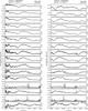 |
Fig. A.1 Line profile developments throughout the whole TIGRE observational campaign of V339 Del. |
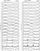 |
Fig. A.1 continued. |
 |
Fig. A.1 continued. |
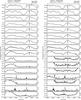 |
Fig. A.1 continued. |
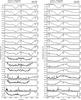 |
Fig. A.1 continued. |
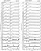 |
Fig. A.1 continued. |
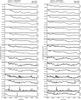 |
Fig. A.1 continued. |
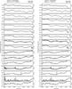 |
Fig. A.1 continued. |
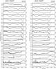 |
Fig. A.1 continued. |
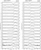 |
Fig. A.1 continued. |
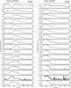 |
Fig. A.1 continued. |
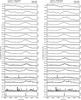 |
Fig. A.1 continued. |
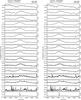 |
Fig. A.1 continued. |
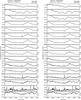 |
Fig. A.1 continued. |
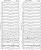 |
Fig. A.1 continued. |
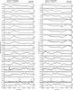 |
Fig. A.1 continued. |
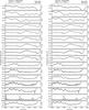 |
Fig. A.1 continued. |
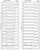 |
Fig. A.1 continued. |
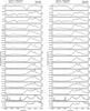 |
Fig. A.1 continued. |
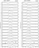 |
Fig. A.1 continued. |
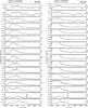 |
Fig. A.1 continued. |
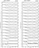 |
Fig. A.1 continued. |
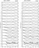 |
Fig. A.1 continued. |
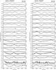 |
Fig. A.1 continued. |
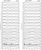 |
Fig. A.1 continued. |
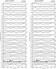 |
Fig. A.1 continued. |
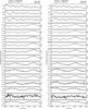 |
Fig. A.1 continued. |
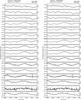 |
Fig. A.1 continued. |
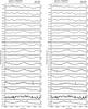 |
Fig. A.1 continued. |
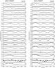 |
Fig. A.1 continued. |
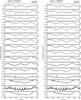 |
Fig. A.1 continued. |
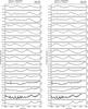 |
Fig. A.1 continued. |
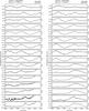 |
Fig. A.1 continued. |
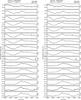 |
Fig. A.1 continued. |
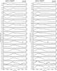 |
Fig. A.1 continued. |
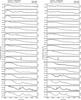 |
Fig. A.1 continued. |
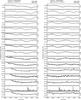 |
Fig. A.1 continued. |
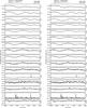 |
Fig. A.1 continued. |
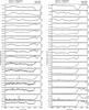 |
Fig. A.1 continued. |
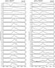 |
Fig. A.1 continued. |
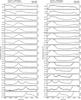 |
Fig. A.1 continued. |
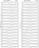 |
Fig. A.1 continued. |
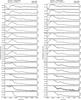 |
Fig. A.1 continued. |
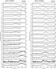 |
Fig. A.1 continued. |
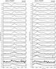 |
Fig. A.1 continued. |
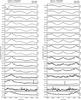 |
Fig. A.1 continued. |
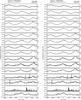 |
Fig. A.1 continued. |
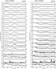 |
Fig. A.1 continued. |
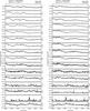 |
Fig. A.1 continued. |
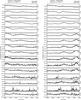 |
Fig. A.1 continued. |
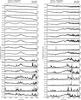 |
Fig. A.1 continued. |
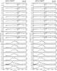 |
Fig. A.1 continued. |
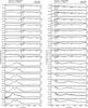 |
Fig. A.1 continued. |
 |
Fig. A.1 continued. |
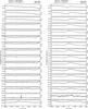 |
Fig. A.1 continued. |
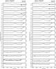 |
Fig. A.1 continued. |
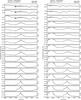 |
Fig. A.1 continued. |
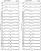 |
Fig. A.1 continued. |
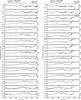 |
Fig. A.1 continued. |
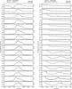 |
Fig. A.1 continued. |
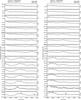 |
Fig. A.1 continued. |
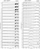 |
Fig. A.1 continued. |
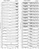 |
Fig. A.1 continued. |
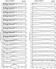 |
Fig. A.1 continued. |
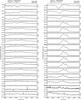 |
Fig. A.1 continued. |
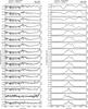 |
Fig. A.1 continued. |
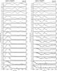 |
Fig. A.1 continued. |
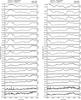 |
Fig. A.1 continued. |
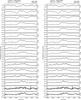 |
Fig. A.1 continued. |
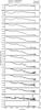 |
Fig. A.1 continued. |
All Tables
All Figures
|
Fig. 1 Lightcurve of V339 Del in the V band. The dots represent daily averages from the AAVSO data. The vertical lines separate the different phases discussed in Sect. 3: A. optically thick; B. transition; C. early nebular; D. late nebular. The triangles mark the TIGRE observations (Table 1). |
| In the text | |
|
Fig. 2a TIGRE/HEROS spectra from days +3 (optically thick phase), +15 (transition phase), +42 (early nebular phase), and +121 (late nebular phase) after discovery. Blue channel. The spectra are blaze-normalized and subsequently normalized to a polynomial instrumental response function. No absolute flux calibration has been applied. Flux is shown on a logarithmic scale to better display the several spectroscopic features. The most relevant lines are numbered in italics, and for their identifications see Table 2. |
| In the text | |
|
Fig. 2b continued − Red channel. |
| In the text | |
|
Fig. 3 Ionized species observed throughout the observational campaign. The dotted vertical lines indicate the different phases introduced in Sect. 3. The full vertical line corresponds to the peak of the soft X-ray emission (details in Sect. 4). |
| In the text | |
|
Fig. 4 On day +3, the two most relevant lines seen here are Hγ and Hδ, both exhibiting P-Cyg-like profiles, while the other species, mainly Fe II, show only narrow absorption features. Later (days +5 and +6) the spectrum consists of a multitude of wide, overlapping emission line profiles. |
| In the text | |
|
Fig. 5 Low ionization stages of heavy elements identified during the optically thick phase (day +3 in this case), with Hζ as a reference. The dotted vertical line marks −660 km s-1 on the radial velocity scale used here. |
| In the text | |
|
Fig. 6 Hα and Hβ development through the whole time span. |
| In the text | |
|
Fig. 7 Development of Fe II 4923.3 Å in the early phase, showing the progression of the minimum of the absorption towards higher negative velocities. The vertical dotted line marks a radial velocity of −660 km s-1, as in Fig. 5. |
| In the text | |
|
Fig. 8 Hδ development during the transition phase. The spectra are normalized to the peak of the line and vertically shifted. |
| In the text | |
|
Fig. 9 From top to bottom, the nebular phase development for Hα 6562 Å, He II 4686,Å and [Fe VII] 6087, showing the re-enhancement of the core of the first two lines and the appearance of the [Fe VII] line. |
| In the text | |
|
Fig. 10 Comparison between V339 Del (day +121) and the ONe nova V959 Mon (day +152), illustrating the absence of [Ne IV] 4714, 4725 Å lines in Nova Del 2013. |
| In the text | |
|
Fig. A.1 Line profile developments throughout the whole TIGRE observational campaign of V339 Del. |
| In the text | |
|
Fig. A.1 continued. |
| In the text | |
|
Fig. A.1 continued. |
| In the text | |
|
Fig. A.1 continued. |
| In the text | |
|
Fig. A.1 continued. |
| In the text | |
|
Fig. A.1 continued. |
| In the text | |
|
Fig. A.1 continued. |
| In the text | |
|
Fig. A.1 continued. |
| In the text | |
|
Fig. A.1 continued. |
| In the text | |
|
Fig. A.1 continued. |
| In the text | |
|
Fig. A.1 continued. |
| In the text | |
|
Fig. A.1 continued. |
| In the text | |
|
Fig. A.1 continued. |
| In the text | |
|
Fig. A.1 continued. |
| In the text | |
|
Fig. A.1 continued. |
| In the text | |
|
Fig. A.1 continued. |
| In the text | |
|
Fig. A.1 continued. |
| In the text | |
|
Fig. A.1 continued. |
| In the text | |
|
Fig. A.1 continued. |
| In the text | |
|
Fig. A.1 continued. |
| In the text | |
|
Fig. A.1 continued. |
| In the text | |
|
Fig. A.1 continued. |
| In the text | |
|
Fig. A.1 continued. |
| In the text | |
|
Fig. A.1 continued. |
| In the text | |
|
Fig. A.1 continued. |
| In the text | |
|
Fig. A.1 continued. |
| In the text | |
|
Fig. A.1 continued. |
| In the text | |
|
Fig. A.1 continued. |
| In the text | |
|
Fig. A.1 continued. |
| In the text | |
|
Fig. A.1 continued. |
| In the text | |
|
Fig. A.1 continued. |
| In the text | |
|
Fig. A.1 continued. |
| In the text | |
|
Fig. A.1 continued. |
| In the text | |
|
Fig. A.1 continued. |
| In the text | |
|
Fig. A.1 continued. |
| In the text | |
|
Fig. A.1 continued. |
| In the text | |
|
Fig. A.1 continued. |
| In the text | |
|
Fig. A.1 continued. |
| In the text | |
|
Fig. A.1 continued. |
| In the text | |
|
Fig. A.1 continued. |
| In the text | |
|
Fig. A.1 continued. |
| In the text | |
|
Fig. A.1 continued. |
| In the text | |
|
Fig. A.1 continued. |
| In the text | |
|
Fig. A.1 continued. |
| In the text | |
|
Fig. A.1 continued. |
| In the text | |
|
Fig. A.1 continued. |
| In the text | |
|
Fig. A.1 continued. |
| In the text | |
|
Fig. A.1 continued. |
| In the text | |
|
Fig. A.1 continued. |
| In the text | |
|
Fig. A.1 continued. |
| In the text | |
|
Fig. A.1 continued. |
| In the text | |
|
Fig. A.1 continued. |
| In the text | |
|
Fig. A.1 continued. |
| In the text | |
|
Fig. A.1 continued. |
| In the text | |
|
Fig. A.1 continued. |
| In the text | |
|
Fig. A.1 continued. |
| In the text | |
|
Fig. A.1 continued. |
| In the text | |
|
Fig. A.1 continued. |
| In the text | |
|
Fig. A.1 continued. |
| In the text | |
|
Fig. A.1 continued. |
| In the text | |
|
Fig. A.1 continued. |
| In the text | |
|
Fig. A.1 continued. |
| In the text | |
|
Fig. A.1 continued. |
| In the text | |
|
Fig. A.1 continued. |
| In the text | |
|
Fig. A.1 continued. |
| In the text | |
|
Fig. A.1 continued. |
| In the text | |
|
Fig. A.1 continued. |
| In the text | |
|
Fig. A.1 continued. |
| In the text | |
|
Fig. A.1 continued. |
| In the text | |
|
Fig. A.1 continued. |
| In the text | |
Current usage metrics show cumulative count of Article Views (full-text article views including HTML views, PDF and ePub downloads, according to the available data) and Abstracts Views on Vision4Press platform.
Data correspond to usage on the plateform after 2015. The current usage metrics is available 48-96 hours after online publication and is updated daily on week days.
Initial download of the metrics may take a while.