© ESO, 2015

1. Introduction and context

Since 1995, more than 1500 exoplanets have been discovered around a wide range of host star types (e.g. Perryman 2011). To date, their mass range spreads from M red dwarfs to intermediate-mass A-type stars. In this context, tidal dissipation in the host star has a strong impact on the orbital configuration of short-period systems. The dissipation in rotating turbulent convective envelopes of low-mass stars is believed to play a crucial role for tidal migration, circularization of orbits, and spin alignment (e.g. Albrecht et al. 2012; Lai 2012; Ogilvie 2014, and references therein for hot-Jupiter systems). In these regions, it is the turbulent friction acting on tidal flows, which dissipates their kinetic energy into heat, that drives the tidal evolution of star-planet systems. In stellar convection zones, tidal flows are constituted of large-scale non-wavelike/equilibrium flows driven by the hydrostatic adjustment of the stellar structure because of the presence of the planetary/stellar companion (Zahn 1966; Remus et al. 2012) and the dynamical tide constituted by inertial waves, their restoring force being the Coriolis acceleration (e.g. Ogilvie & Lin 2007). In this framework, both the structure and rotation of stars strongly varies along their evolution (e.g. Siess et al. 2000; Gallet & Bouvier 2013, 2015). Moreover, as reported by Ogilvie (2014), observations of star-planet and binary-star systems show that tidal dissipation varies over several orders of magnitude. Therefore, one of the key questions that must be addressed is, how does tidal dissipation in the convective envelope of low-mass stars vary as a function of stellar mass, evolutionary stage, and rotation?

In this work, we study the variations of the frequency-averaged tidal dissipation in stellar convective envelopes as a function of the mass, the age, and the rotation of stars. In Sect. 2, we introduce the assumptions and the formalism that allows us to analytically evaluate this quantity as a function of the structure and rotation of stars (Ogilvie 2013). In Sect. 3, we compute it as a function of stellar mass and evolutionary stage at fixed angular velocity using grids of stellar models for stars from 0.4 to 1.4 M_⊙. Next, we discuss the impact of the rotational evolution of stars. In Sect. 4, we present our conclusions and the perspectives of this work.

2. Tidal dissipation modelling

To analytically evaluate the frequency-averaged tidal dissipation in the convective envelope of low-mass stars, we adopt a simplified two-layer model as in Ogilvie (2013; see also Penev et al. 2014, and Fig. 1). In this modelling, both the radiative core and the convective envelope are assumed to be homogeneous with respective constant densities ρ_c and ρ_e for the sake of simplicity. This model features a star A of mass M_s and mean radius R_s hosting a point-mass tidal perturber B of mass m orbiting with a mean motion n. The convective envelope of A is assumed to be in moderate solid-body rotation with an angular velocity Ω so that ${\mathit{ϵ}}^{\mathrm{2}}\mathrm{\equiv }{\left(\mathrm{\Omega }\mathit{/}\sqrt{\mathrm{𝒢}{\mathit{M}}_{\mathrm{s}}\mathit{/}{\mathit{R}}_{\mathrm{s}}^{\mathrm{3}}}\right)}^{\mathrm{2}}\mathrm{=}{\left(\mathrm{\Omega }\mathit{/}{\mathrm{\Omega }}_{\mathrm{c}}\right)}^{\mathrm{2}}\mathrm{\ll }\mathrm{1}$¹, where Ω_c is the critical angular velocity and is the gravitational constant. It surrounds the radiative core of radius R_c and mass M_c.

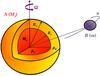Fig. 1 Two-layer low-mass star A of mass Ms and mean radius Rs and point-mass tidal perturber B of mass m orbiting with a mean motion n. The radiative core of radius Rc, mass Mc, and density ρc is surrounded by the convective envelope of density ρe.

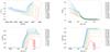Fig. 2 Top-left: track of evolution of stars from 0.4 to 1.4 M⊙ in the Hertzsprung-Russell diagram that gives the luminosity (L) as a function of effective temperature (Teff) (red, orange, green, dark blue, and cyan lines correspond to M-, K-, G-, F-, and A-type stars, respectively). Top-right: evolution of the stellar radius Rs of stars from 0.4 to 1.4 M⊙ as a function of time. Bottom-left: evolution of the radius aspect ratio α = Rc/Rs of stars from 0.4 to 1.4 M⊙ as a function of time. Bottom-right: evolution of the mass aspect ratio β = Mc/Ms of stars from 0.4 to 1.4 M⊙ as a function of time.

Tidal dissipation in the external convection zone of A originates from the excitation by B of inertial waves, which have the Coriolis acceleration as restoring force. They are damped by the turbulent friction, which is modelled using a turbulent viscosity (see Ogilvie & Lesur 2012, and references therein). Its analytical evaluation in our two-layer model was conducted by Ogilvie (2013) who assumed a homogeneous and incompressible convective envelope² surrounding a homogeneous and stable fluid core where no dissipation occurs. The solutions of the system of dynamical equations for the envelope written in the co-rotating frame are separated into a non-wavelike part (with subscripts _nw), which corresponds to the immediate hydrostatic adjustment to the external tidal potential (U), and a wavelike part (with subscript _w) driven by the action of the Coriolis acceleration on the non-wavelike part (see Appendix A and Ogilvie 2013). The kinetic energy of the wavelike part of the solution can be derived without solving the whole system of equations, thanks to an impulsive calculation. It is dissipated after a finite time and allows us to compute the frequency-averaged tidal dissipation given in Ogilvie (2013; Eq. (B3))³, $\begin{array}{ccc}{⟨\mathrm{𝒟}⟩}_{\mathit{\omega }}\mathrm{=}{\mathrm{\int }}_{\mathrm{-}\mathrm{\infty }}^{\mathrm{+}\mathrm{\infty }}\mathrm{Im}\mathrm{[}{\mathit{k}}_{\mathrm{2}}^{\mathrm{2}}\mathrm{(}\mathit{\omega }{\mathrm{)}}^{\mathrm{]}}\hspace{0.17em}\frac{\mathrm{d}\mathit{\omega }}{\mathit{\omega }}\mathrm{=}\frac{\mathrm{100}\mathit{\pi }}{\mathrm{63}}{\mathit{ϵ}}^{\mathrm{2}}\left(\frac{{\mathit{\alpha }}^{\mathrm{5}}}{\mathrm{1}\mathrm{-}{\mathit{\alpha }}^{\mathrm{5}}}\right){\left(\mathrm{1}\mathrm{-}\mathit{\gamma }\right)}^{\mathrm{2}}& & \\ & & \mathrm{\times }{\mathrm{(}\mathrm{1}\mathrm{-}{\mathit{\alpha }}^{\mathrm{)}}}^{\mathrm{4}}{\left(\mathrm{1}\mathrm{+}\mathrm{2}\mathit{\alpha }\mathrm{+}\mathrm{3}{\mathit{\alpha }}^{\mathrm{2}}\mathrm{+}\frac{\mathrm{3}}{\mathrm{2}}{\mathit{\alpha }}^{\mathrm{3}}\right)}^{\mathrm{2}}\left[\mathrm{1}\mathrm{+}\left(\frac{\mathrm{1}\mathrm{-}\mathit{\gamma }}{\mathit{\gamma }}\right){\mathit{\alpha }}^{\mathrm{3}}\right]\\ & & \end{array}$(1)with $\mathit{\alpha }\mathrm{=}\frac{{\mathit{R}}_{\mathrm{c}}}{{\mathit{R}}_{\mathrm{s}}}\mathrm{,} \mathit{\beta }\mathrm{=}\frac{{\mathit{M}}_{\mathrm{c}}}{{\mathit{M}}_{\mathrm{s}}} \mathrm{and} \mathit{\gamma }\mathrm{=}\frac{{\mathit{\rho }}_{\mathrm{e}}}{{\mathit{\rho }}_{\mathrm{c}}}\mathrm{=}\frac{{\mathit{\alpha }}^{\mathrm{3}}\left(\mathrm{1}\mathrm{-}\mathit{\beta }\right)}{\mathit{\beta }\left(\mathrm{1}\mathrm{-}{\mathit{\alpha }}^{\mathrm{3}}\right)}\mathit{<}\mathrm{1.}$(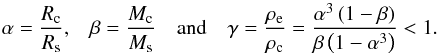2)We introduce the tidal frequency ω = sn − mΩ (with s ∈ Z^ZZ) and the Love number ${\mathit{k}}_{\mathit{l}}^{\mathit{m}}$, associated with the ${\mathrm{(}}^{}\mathit{l,}{\mathit{m}}^{\mathrm{)}}$ component of the time-dependent tidal potential U that corresponds to the spherical harmonic ${\mathit{Y}}_{\mathit{l}}^{\mathit{m}}$. It quantifies at the surface of the star A (r = R_s) the ratio of the tidal perturbation of its self-gravity potential over the tidal potential. In the case of a dissipative fluid as in convective envelopes, it is a complex quantity that depends on the tidal frequency with a real part that accounts for the energy stored in the tidal perturbation, while the imaginary part accounts for the energy losses (e.g. Remus et al. 2012). We note that $\mathrm{Im}{}^{\mathrm{[}}\mathit{k}_{\mathit{l}}^{\mathit{m}}\mathrm{(}\mathit{\omega }{\mathrm{\left)}}^{\mathrm{\right]}}$ is proportional to sgn(ω) and can be expressed in terms of the tidal quality factor ${\mathit{Q}}_{\mathit{l}}^{\mathit{m}}\mathrm{\left(}\mathit{\omega }\mathrm{\right)}$ or equivalently the tidal angle ${\mathit{\delta }}_{\mathit{l}}^{\mathit{m}}\mathrm{\left(}\mathit{\omega }\mathrm{\right)}$, which both depend on the tidal frequency: ${{\mathit{Q}}_{\mathit{l}}^{\mathit{m}}\mathrm{\left(}\mathit{\omega }\mathrm{\right)}}^{-1}\mathrm{=}\mathrm{sgn}\mathrm{\left(}\mathit{\omega }\mathrm{\right)}\hspace{0.17em}{\left|{\mathit{k}}_{\mathit{l}}^{\mathit{m}}\mathrm{\left(}\mathit{\omega }\mathrm{\right)}\right|}^{-1}\hspace{0.17em}\mathrm{Im}\mathrm{\left[}{\mathit{k}}_{\mathit{l}}^{\mathit{m}}\mathrm{\right(}\mathit{\omega }{\mathrm{\left)}}^{\mathrm{\right]}}\mathrm{=}\sin \mathrm{[}\mathrm{2}\hspace{0.17em}{\mathit{\delta }}_{\mathit{l}}^{\mathit{m}}\mathrm{(}\mathit{\omega }{\mathrm{\left)}}^{\mathrm{\right]}}\mathit{.}$(3)Here we choose to consider the simplest case of a coplanar system for which the tidal potential (U) reduces to the component (l = 2,m = 2), as well as the quadrupolar response of A. To unravel the impact of the variation of stellar internal structure, we introduce a first frequency-averaged dissipation at fixed normalized angular velocity $⟨\mathrm{𝒟}⟩\begin{array}{c}\mathrm{\Omega }\\ \mathit{\omega }\end{array}\mathrm{=}{\mathit{ϵ}}^{-2}{⟨\mathrm{𝒟}⟩}_{\mathit{\omega }}\mathrm{=}{\mathit{ϵ}}^{-2}{\mathrm{⟨}\mathrm{Im}{\mathrm{\left[}{\mathit{k}}_{\mathrm{2}}^{\mathrm{2}}\mathrm{\right(}\mathit{\omega }{\mathrm{\left)}}^{\mathrm{\right]}}}^{\mathrm{⟩}}}_{\mathit{\omega }}\mathit{,}$(4)which depends on α and β only, and a second frequency-averaged dissipation $⟨\mathrm{𝒟̂}⟩\begin{array}{c}\mathrm{\Omega }\\ \mathit{\omega }\end{array}\mathrm{=}{\mathit{ϵ̂}}^{-2}{⟨\mathrm{𝒟}⟩}_{\mathit{\omega }}\mathrm{=}{\left(\frac{{\mathit{M}}_{\mathrm{s}}}{{\mathit{M}}_{\mathrm{\odot }}}\right)}^{-1}{\left(\frac{{\mathit{R}}_{\mathrm{s}}}{{\mathit{R}}_{\mathrm{\odot }}}\right)}^{\mathrm{3}}⟨\mathrm{𝒟}⟩\begin{array}{c}\mathrm{\Omega }\\ \mathit{\omega }\end{array}\mathit{,}$(5)where ${\mathit{ϵ̂}}^{\mathrm{2}}\mathrm{\equiv }{\left(\mathrm{\Omega }\mathit{/}\sqrt{\mathrm{𝒢}{\mathit{M}}_{\mathrm{\odot }}\mathit{/}{\mathit{R}}_{\mathrm{\odot }}^{\mathrm{3}}}\right)}^{\mathrm{2}}\mathrm{=}{\left(\mathrm{\Omega }\mathit{/}{\mathrm{\Omega }}_{\mathrm{c}}^{\mathrm{\odot }}\right)}^{\mathrm{2}}$ (M_⊙, R_⊙, and ${\mathrm{\Omega }}_{\mathrm{c}}^{\mathrm{\odot }}$ being the solar mass, radius, and critical angular velocity), which also allows us to take into account the dependences on the radius (R_s) variations and on the mass (M_s). We note that these quantities being averaged in frequency, the complicated frequency-dependence of the dissipation in a spherical shell (Ogilvie & Lin 2007) is filtered out. The dissipation at a given frequency could thus be larger or smaller than its averaged value () by several orders of magnitude. Moreover, constitutes a lower bound of the typical dissipation in the whole star since it is also necessary to take into account the damping of tidal gravito-inertial waves in radiation zones (Ivanov et al. 2013).

3. Tidal dissipation along stellar evolution

3.1. Grids of models for low-mass stars

To study the variation of tidal dissipation in the convective envelope of low-mass stars along their evolution in the theoretical framework presented above we need to compute the stellar radius (R_s) and the mass and aspect ratios (respectively α and β) as functions of time. We use grids of stellar models from 0.4 to 1.4 M_⊙ for a metallicity Z = 0.02 computed by Siess et al. (2000) using the STAREVOL code. These stellar models solve, at the zeroth order, the hydrostatic and energetic spherical balances using the relevant equation of state and description of stellar atmospheres (a complete description of the STAREVOL code is given in Siess et al. 2000). They allow us to follow the evolution of stars and of their structure along their evolutionary tracks in the Hetzsprung-Russell diagram (Fig. 2, top left panel). In this work, we choose to focus on the pre-main sequence, main sequence, and sub-giant phases of evolution (hereafter PMS, MS, and SG). In Fig. 2 (top right panel), the variation of the radius of the star (R_s) is plotted as a function of time. For every star, we identify the three well-known phases: i) during the PMS, a star is in contraction and its radius (R_s) decreases; ii) on the MS it reaches an almost constant value until the beginning of the SG phase; iii) on the SG phase, the star’s envelope begins to expand and R_s increases. As was seen in Sect. 2., the important structural properties to compute for tidal dissipation are also the mass and aspect ratios relative to the radiative core on which tidal inertial waves propagating in the convective envelope can reflect, leading potentially to wave attractors where strong dissipation may occur (e.g. Ogilvie & Lin 2007; Goodman & Lackner 2009). In Fig. 2, we plot the temporal evolution of α and β for the different stellar masses studied here (respectively in the bottom left and bottom right panels). After a first phase where the star is completely convective on the Hayashi phase, the central radiative core grows both in radius and mass along the PMS. Next, for a star with M_s ≥ 0.5 M_⊙, both α and β reach a value on the zero age main sequence (ZAMS) that stays almost constant along the MS. For example, in the case of a 1 M_⊙ star we recover the usual solar values α ≈ 0.71 and β ≈ 0.98. Both α and β increase with M_s on the MS. Finally, when a star reaches its SG phase, both α and β decrease because of the simultaneous extension of the convective envelope and contraction of the radiative core.

3.2. Time evolution of tidal dissipation as a function of stellar mass and evolutionary stage

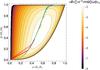Fig. 3 Variation of $⟨\mathrm{𝒟}⟩\begin{array}{c}\mathrm{\Omega }\\ \mathit{\omega }\end{array}\mathrm{=}{\mathit{ϵ}}^{-2}{{}^{\mathrm{⟨}}\mathrm{Im}{{}^{\mathrm{[}}\mathit{k}_{2_{}}^{2^{}}\mathrm{(}\mathit{\omega }{\mathrm{\left)}}^{\mathrm{\right]}}}^{\mathrm{⟩}}}_{\mathit{\omega }}$ as a function of aspect and mass ratios (α and β, respectively) in colour scales. Evolutionary tracks of stars from 0.4 to 1.4 M⊙ in the (α,β) plane (the colours are the same as in Fig. 2).

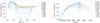Fig. 4 Evolution of the frequency-averaged tidal dissipation at fixed normalized angular velocity, $⟨\mathrm{𝒟̂}⟩\begin{array}{c}\mathrm{\Omega }\\ \mathit{\omega }\end{array}\mathrm{=}{\mathit{ϵ̂}}^{-2}{{}^{\mathrm{⟨}}\mathrm{Im}{{}^{\mathrm{[}}\mathit{k}_{2_{}}^{2^{}}\mathrm{(}\mathit{\omega }{\mathrm{\left)}}^{\mathrm{\right]}}}^{\mathrm{⟩}}}_{\mathit{\omega }}$, as a function of time (left panel) and effective temperature (right panel) for stellar masses (Ms) from 0.4 to 1.4 M⊙ (the colours are the same as in Fig. 2).

After defining the phases of the structural evolution of low-mass stars, we have to compute the corresponding evolution of the dissipation of the kinetic energy of tidal inertial waves in their convective envelope as a function of time. In Fig. 3, we represent i) the intensity of the first frequency-averaged dissipation at fixed normalized angular velocity ($⟨\mathrm{𝒟}⟩\begin{array}{c}\mathrm{\Omega }\\ \mathit{\omega }\end{array}$; see Eq. (4)) as a function of α and β only in colour scales and ii) the position of the couples (α,β) along the evolution of stars for stellar masses from 0.4 to 1.4 M_⊙. On the one hand, $⟨\mathrm{𝒟}⟩\begin{array}{c}\mathrm{\Omega }\\ \mathit{\omega }\end{array}$ presents a maximum in an island region around (α_max ≈ 0.571, β_max ≈ 0.501). On the other hand, stars of different masses have a different evolution of their internal tidal dissipation in their envelope because of their different structural evolution. First, all stars have an increase of $⟨\mathrm{𝒟}⟩\begin{array}{c}\mathrm{\Omega }\\ \mathit{\omega }\end{array}$ during the beginning of their PMS until they reach a position in the diagram close to (α_max, β_max) because of the formation and the growth of their radiative core. Then, $⟨\mathrm{𝒟}⟩\begin{array}{c}\mathrm{\Omega }\\ \mathit{\omega }\end{array}$ has an evolution that is a direct function of stellar mass. For 0.4 M_⊙ M-type stars, the radiative core has an evolution where it finally disappears. Therefore, the configuration converges on the MS to the case of fully convective stars with the weak dissipation of normal inertial modes (Wu 2005). For stars from 0.5 M_⊙ to 1.4 M_⊙ masses, the evolution is different. After they have reached their position closest to (α_max, β_max) in the diagram, they evolve to a position (α_MS, β_MS) where they stay during almost the whole MS because of the weak evolution of these quantities. Since α_MS and β_MS are increasing functions of the stellar mass, $⟨\mathrm{𝒟}⟩\begin{array}{c}\mathrm{\Omega }\\ \mathit{\omega }\end{array}$ – which is almost constant on the MS – decreases from K- to A-type stars. However, the evolution of R_s must also be taken into account. Therefore, the evolution of $\mathrm{⟨}\mathrm{𝒟̂}{\mathrm{⟩}}_{\mathit{\omega }}^{\mathrm{\Omega }}$ (see Eq. (5)) as a function of time (left panel) and of the effective temperature (right panel) are given in Fig. 4 taking into account the simultaneous variations of α, β, and R_s. We recover the two phases of the evolution of the dissipation. On the PMS, it increases towards the maximum value, which grows with stellar mass, corresponding to the region around (α_max, β_max) for all stellar masses. The time coordinate of this maximum is smaller if stellar mass is higher because of the corresponding shorter life-time of the star. Then, the dissipation decreases to rapidly reach its almost constant value on the MS. As already pointed out, and expected from observational constraints (e.g. Albrecht et al. 2012) and previous theoretical works (Ogilvie & Lin 2007; Barker & Ogilvie 2009)⁴, it decreases with stellar mass from 0.6 M_⊙ K-type to A-type stars by several orders of magnitude (≈3 between 0.6 and 1.4 M_⊙) because of the variation in the thickness of the convective envelope, which becomes thinner. Finally, for higher mass stars, we can see a final increase of $\mathrm{⟨}\mathrm{𝒟̂}{\mathrm{⟩}}_{\mathit{\omega }}^{\mathrm{\Omega }}$ because of the simultaneous extension of their convective envelope and contraction of their radiative core during their SG phase leading again the star towards the region of maximum dissipation in the (α,β) plane.

3.3. Impact of the rotational evolution of stars

It is also crucial to discuss consequences of the rotational evolution of low-mass stars. As we know from observational works and related modelling (e.g. Gallet & Bouvier 2013, 2015, and references therein), their rotation follows three main phases of evolution: i) stars are trapped in co-rotation with the surrounding circumstellar disk; ii) because of the contraction of stars on the PMS (e.g. Fig. 3, top left panel) their rotation (and thus ϵ) increases; and iii) stars are braked on the MS because of the torque applied by pressure-driven stellar winds (e.g. Réville et al. 2015, and references therein) and ϵ decreases. As a detailed computation of stellar rotating models is beyond the scope of the present work owing to the complex internal and external mechanisms that must be taken into account, we will not evaluate here the variation of tidal dissipation because of the simultaneous evolution of stellar internal structure and rotation. However, from results obtained by Gallet & Bouvier (2013, 2015), we can easily infer that increases during the PMS because of the growth of the radiative core and of the angular velocity. From Fig. 5 in Gallet & Bouvier (2015), we can see that in the case of the 0.5 M_⊙ star this growth will be simultaneous. On the MS, decreases because of the evolution of the structure of the star and of its braking by stellar winds. As demonstrated before, the value of M_s is determinant.

4. Conclusions

All low-mass stars have an increase in the frequency-averaged tidal dissipation for a fixed angular velocity in their convective envelope for tidal frequencies lying within the range [−2Ω,2Ω] so that inertial waves can be excited until they reach a critical

aspect and mass ratios close to (α_max,β_max) during the PMS. Next, they evolve on the MS to an asymptotic value that reaches a maximum for 0.6 M_⊙ K-type stars and then decreases by several orders of magnitude with increasing stellar mass. Finally, the rotational evolution of low-mass stars strengthens the importance of tidal dissipation during the PMS for star-planet and multiple star systems as pointed out by Zahn & Bouchet (1989).

In the near future, it would be important to improve the physics of dissipation in stellar convection zones by taking into account density stratification, differential rotation, magnetic field and non-linear effects, and related possible instabilities (e.g. Baruteau & Rieutord 2013; Schmitt 2010; Favier et al. 2014). Moreover, it will be necessary to include results obtained for the dissipation of tidal gravito-inertial waves in stellar radiative cores (Ivanov et al. 2013) to obtain a complete picture (Guillot et al. 2014). Finally, it will be interesting to explore advanced phases of stellar evolution.

Online material

Appendix A: Dynamical equations for tidal flows in convective envelopes

The solutions of the system of dynamical equations for the envelope written in the co-rotating frame are separated into a non-wavelike part (with subscripts _nw), which corresponds to the immediate hydrostatic adjustment to the external tidal potential (U), and a wavelike part (with subscript _w) driven by the action of the Coriolis acceleration on the non-wavelike part, 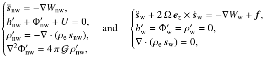$\{\begin{array}{c}\\ \\ \\ \\ \end{array}\mathrm{and} \{\begin{array}{c}\\ \\ \\ \end{array}$(A.1)

where s is the displacement, e_z the unit vector along the rotation axis, h the specific enthalpy, and Φ is the self-gravitational potential of A. Primed variables denote an Eulerian perturbation in relation to the unperturbed state with unprimed variables. We note that U being of the first order in tidal amplitude, it appears in perturbation equations. Finally, W ≡ W_nw + W_w = h′ + Φ′ + U, while ${f}\mathrm{=}\mathrm{-}\mathrm{2}\hspace{0.17em}\mathrm{\Omega }\hspace{0.17em}{{e}}_{\mathit{z}}\mathrm{\times }\dot{{s}}{}_{\mathrm{nw}}$ is the acceleration driving the wavelike part of the solution.

Acknowledgments

The author is grateful to the referee, A. Barker, for his detailed review, which has allowed us to improve the paper. This work was supported by the Programme National de Planétologie (CNRS/INSU) and the CoRoT-CNES grant at Service d’Astrophysique (CEA-Saclay). S.M. dedicates this article to J. Abrassart.

References

All Figures

	Fig. 1 Two-layer low-mass star A of mass Ms and mean radius Rs and point-mass tidal perturber B of mass m orbiting with a mean motion n. The radiative core of radius Rc, mass Mc, and density ρc is surrounded by the convective envelope of density ρe.
In the text

Fig. 2 Top-left: track of evolution of stars from 0.4 to 1.4 M⊙ in the Hertzsprung-Russell diagram that gives the luminosity (L) as a function of effective temperature (Teff) (red, orange, green, dark blue, and cyan lines correspond to M-, K-, G-, F-, and A-type stars, respectively). Top-right: evolution of the stellar radius Rs of stars from 0.4 to 1.4 M⊙ as a function of time. Bottom-left: evolution of the radius aspect ratio α = Rc/Rs of stars from 0.4 to 1.4 M⊙ as a function of time. Bottom-right: evolution of the mass aspect ratio β = Mc/Ms of stars from 0.4 to 1.4 M⊙ as a function of time.

In the text

Fig. 3 Variation of $⟨\mathrm{𝒟}⟩\begin{array}{c}\mathrm{\Omega }\\ \mathit{\omega }\end{array}\mathrm{=}{\mathit{ϵ}}^{-2}{{}^{\mathrm{⟨}}\mathrm{Im}{{}^{\mathrm{[}}\mathit{k}_{2_{}}^{2^{}}\mathrm{(}\mathit{\omega }{\mathrm{\left)}}^{\mathrm{\right]}}}^{\mathrm{⟩}}}_{\mathit{\omega }}$ as a function of aspect and mass ratios (α and β, respectively) in colour scales. Evolutionary tracks of stars from 0.4 to 1.4 M⊙ in the (α,β) plane (the colours are the same as in Fig. 2).

In the text

Fig. 4 Evolution of the frequency-averaged tidal dissipation at fixed normalized angular velocity, $⟨\mathrm{𝒟̂}⟩\begin{array}{c}\mathrm{\Omega }\\ \mathit{\omega }\end{array}\mathrm{=}{\mathit{ϵ̂}}^{-2}{{}^{\mathrm{⟨}}\mathrm{Im}{{}^{\mathrm{[}}\mathit{k}_{2_{}}^{2^{}}\mathrm{(}\mathit{\omega }{\mathrm{\left)}}^{\mathrm{\right]}}}^{\mathrm{⟩}}}_{\mathit{\omega }}$, as a function of time (left panel) and effective temperature (right panel) for stellar masses (Ms) from 0.4 to 1.4 M⊙ (the colours are the same as in Fig. 2).

In the text

References

- Albrecht, S., Winn, J. N., Johnson, J. A., et al. 2012, ApJ, 757, 18 [NASA ADS] [CrossRef] [Google Scholar]
- Barker, A. J., & Ogilvie, G. I. 2009, MNRAS, 395, 2268 [NASA ADS] [CrossRef] [Google Scholar]
- Baruteau, C., & Rieutord, M. 2013, J. Fluid Mech., 719, 47 [Google Scholar]
- Favier, B., Barker, A. J., Baruteau, C., & Ogilvie, G. I. 2014, MNRAS, 439, 845 [NASA ADS] [CrossRef] [Google Scholar]
- Gallet, F., & Bouvier, J. 2013, A&A, 556, A36 [NASA ADS] [CrossRef] [EDP Sciences] [Google Scholar]
- Gallet, F., & Bouvier, J. 2015, A&A, 577, A98 [NASA ADS] [CrossRef] [EDP Sciences] [Google Scholar]
- Goodman, J., & Lackner, C. 2009, ApJ, 696, 2054 [NASA ADS] [CrossRef] [Google Scholar]
- Guillot, T., Lin, D. N. C., Morel, P., Havel, M., & Parmentier, V. 2014, EAS Pub. Ser., 65, 327 [CrossRef] [EDP Sciences] [Google Scholar]
- Ivanov, P. B., Papaloizou, J. C. B., & Chernov, S. V. 2013, MNRAS, 432, 2339 [NASA ADS] [CrossRef] [Google Scholar]
- Lai, D. 2012, MNRAS, 423, 486 [NASA ADS] [CrossRef] [Google Scholar]
- Ogilvie, G. I. 2013, MNRAS, 429, 613 [NASA ADS] [CrossRef] [Google Scholar]
- Ogilvie, G. I. 2014, ARA&A, 52, 171 [Google Scholar]
- Ogilvie, G. I., & Lesur, G. 2012, MNRAS, 422, 1975 [NASA ADS] [CrossRef] [Google Scholar]
- Ogilvie, G. I., & Lin, D. N. C. 2007, ApJ, 661, 1180 [NASA ADS] [CrossRef] [Google Scholar]
- Penev, K., Zhang, M., & Jackson, B. 2014, PASP, 126, 553 [NASA ADS] [CrossRef] [Google Scholar]
- Perryman, M. 2011, The Exoplanet Handbook (Cambridge University Press) [Google Scholar]
- Remus, F., Mathis, S., & Zahn, J.-P. 2012, A&A, 544, A132 [NASA ADS] [CrossRef] [EDP Sciences] [Google Scholar]
- Réville, V., Brun, A. S., Matt, S. P., Strugarek, A., & Pinto, R. F. 2015, ApJ, 798, 116 [NASA ADS] [CrossRef] [Google Scholar]
- Schmitt, D. 2010, Geophys. Astrophys. Fluid Dyn., 104, 135 [NASA ADS] [CrossRef] [Google Scholar]
- Siess, L., Dufour, E., & Forestini, M. 2000, A&A, 358, 593 [Google Scholar]
- Wu, Y. 2005, ApJ, 635, 688 [NASA ADS] [CrossRef] [Google Scholar]
- Zahn, J. P. 1966, Ann. Astrophys., 29, 489 [NASA ADS] [Google Scholar]
- Zahn, J.-P., & Bouchet, L. 1989, A&A, 223, 112 [Google Scholar]