| Issue |
A&A
Volume 580, August 2015
|
|
|---|---|---|
| Article Number | A110 | |
| Number of page(s) | 16 | |
| Section | Numerical methods and codes | |
| DOI | https://doi.org/10.1051/0004-6361/201526247 | |
| Published online | 11 August 2015 | |
Astrophysical fluid simulations of thermally ideal gases with non-constant adiabatic index: numerical implementation
1
Dipartimento di FisicaUniversità di Torino, via Pietro Giuria 1, 10125
Torino, Italy
e-mail: This email address is being protected from spambots. You need JavaScript enabled to view it.
2
INAF, Osservatorio Astronomico di Torino,
Strada Osservatorio 20,
10025
Pino Torinese,
Italy
Received:
2
April
2015
Accepted:
4
June
2015
Abstract
Context. An equation of state (EoS) is a relation between thermodynamic state variables and it is essential for closing the set of equations describing a fluid system. Although an ideal EoS with a constant adiabatic index Γ is the preferred choice owing to its simplistic implementation, many astrophysical fluid simulations may benefit from a more sophisticated treatment that can account for diverse chemical processes.
Aims. In the present work we first review the basic thermodynamic principles of a gas mixture in terms of its thermal and caloric EoS by including effects like ionization, dissociation, and temperature dependent degrees of freedom such as molecular vibrations and rotations. The formulation is revisited in the context of plasmas that are either in equilibrium conditions (local thermodynamic- or collisional excitation-equilibria) or described by non-equilibrium chemistry coupled to optically thin radiative cooling. We then present a numerical implementation of thermally ideal gases obeying a more general caloric EoS with non-constant adiabatic index in Godunov-type numerical schemes.
Methods. We discuss the necessary modifications to the Riemann solver and to the conversion between total energy and pressure (or vice versa) routinely invoked in Godunov-type schemes. We then present two different approaches for computing the EoS. The first employs root-finder methods and it is best suited for EoS in analytical form. The second is based on lookup tables and interpolation and results in a more computationally efficient approach, although care must be taken to ensure thermodynamic consistency.
Results. A number of selected benchmarks demonstrate that the employment of a non-ideal EoS can lead to important differences in the solution when the temperature range is 500−104 K where dissociation and ionization occur. The implementation of selected EoS introduces additional computational costs although the employment of lookup table methods (when possible) can significantly reduce the overhead by a factor of ~ 3−4.
Key words: equation of state / methods: numerical / atomic processes / molecular processes / shock waves
© ESO, 2015
1. Introduction
An equation of state (EoS) is a relationship between state variables of a thermodynamic system under certain physical conditions. Such a constitutive equation provides the necessary closure for a complete mathematical description of a fluid system in addition to the conservation laws of mass, momentum and energy. Numerical simulations of astrophysical systems such as interstellar medium (ISM), planetary atmospheres, stellar evolution, jets and outflows, require the inter-play of various thermal, radiative and chemical processes. For such complex systems, using a simple ideal (or an isothermal) EoS would be considered a serious limitation. A consistent description for such systems demands the use of a general EoS that can account for thermal and chemical processes.
For example, the thermodynamic state of the gas plays a pivotal role in governing the fragmentation of self-gravitating and turbulent molecular clouds (e.g., Spaans & Silk 2000; Li et al. 2003; Jappsen et al. 2005). The balance between heating and cooling in molecular clouds is approximated by using a poly-tropic EoS, p ∝ ρΓ. Multiple smoothed particle hydrodynamical simulations with different adiabatic indices, 0.2 < Γ < 1.4 (Spaans & Silk 2000) were used to show that the degree of fragmentation decreases with increasing value of Γ (Li et al. 2003). Jappsen et al. (2005) showed that the thermal properties of the gas determine the stellar mass function (IMF) using a piecewise poly-tropic EoS. Such empirical forms of EoS in general depend on chemical abundances and complex atomic and molecular physics.
Numerical simulations studying thermo-chemical evolution of early structure formation used an effective adiabatic index, Γeff, to relate internal energy with thermal pressure (e.g., Yoshida et al. 2006; Glover & Abel 2008). The value of Γeff is estimated from number fractions of chemical species treating the chemical composition as an ideal mixture. In the context of disk instability leading to formation of gas giant planets, Boley et al. (2007) pointed out the importance of incorporating isotopic forms of molecular hydrogen, H2, as well the molecular physics (rotation and vibration) under thermodynamic equilibrium in the estimate of internal energy. A more complex EoS taking into account ionization of atomic hydrogen, helium and radiation along with molecular dissociations is used to study the envelopes of young planetary cores (D’Angelo & Bodenheimer 2013).
From the computational perspective, procedures to treat dynamics of astrophysical plasmas with a general EoS have been developed by appropriately modifying the Riemann solver as described, e.g., by Colella & Glaz (1985), Glaister (1988b,a), Menikoff & Plohr (1989), Liou et al. (1990), Fedkiw et al. (1997), Hu et al. (2009). Similarly, numerical codes like FLASH (Fryxell et al. 2000) and CASTRO (Almgren et al. 2010) have implemented electron-positron EoS (Timmes & Swesty 2000) using high-order polynomials as interpolating functions. Such an EoS based on tabulated Helmholtz free energy is employed in the study of stellar evolution and supernovae. Falle & Raga (1993, 1995) incorporated local thermodynamic equilibrium (LTE) effects to model partially ionized hydrogen gas using Saha Equations to study variable knots produced in stellar jets.
The goal of this paper is to outline a consistent numerical framework for the implementation of a more general equation of state in the context of the magnetohydrodynamics (MHD) equations. Our formulation accounts for different physical processes such as atomic ionization and recombination, molecular dissociation, etc., and it is suitable under equilibrium conditions (local thermodynamic or collisional ionization equilibria) and for non-equilibrium optically thin radiative cooling (Teşileanu et al. 2008). The numerical method is implemented as part of the PLUTO code (Mignone et al. 2007) and it is built while ensuring thermodynamical consistency, accuracy and computational efficiency.
Our starting point are the ideal MHD equations written in conservation form, ![Mathematical equation: \begin{eqnarray} \label{eq:mhd_rho} &&\DS \pd{\rho}{t} + \nabla\cdot\left(\rho\vec{v}\right) = 0 \\ \label{eq:mhd_mom} &&\DS \pd{\vec{(\rho\vec{v})}}{t} + \nabla\cdot\left( \rho\vec{v}\vec{v}^T - \vec{B}\vec{B}^T\right) + \nabla p_t = 0 \\ \label{eq:mhd_B} &&\DS \pd{\vec{B}}{t} - \nabla\times\left(\vec{v}\times\vec{B}\right) = \vec{0}\, \\ \label{eq:mhd_E} &&\DS \pd{E}{t} + \nabla\cdot\left[ \left(E + p_t\right)\vec{v} - \left(\vec{v}\cdot\vec{B}\right)\vec{B}\right] = \Lambda \\ \label{eq:mhd_X} &&\DS \pd{(\rho X_k)}{t} + \nabla\cdot\left(\rho X_k\vec{v}\right) = S_k, \end{eqnarray}](/articles/aa/full_html/2015/08/aa26247-15/aa26247-15-eq8.png) where
ρ is the mass
density, v is the fluid velocity, B is the
magnetic field, and pt = p +
B2/ 2 is
the total pressure accounting for thermal (p) and magnetic (B2/
2) contributions. The total energy density E is given by
where
ρ is the mass
density, v is the fluid velocity, B is the
magnetic field, and pt = p +
B2/ 2 is
the total pressure accounting for thermal (p) and magnetic (B2/
2) contributions. The total energy density E is given by  (6)An additional EoS
relating the internal energy density ρe with p and ρ must be specified. This issue is addressed in Sect.
2. Dissipative effects have been neglected for the
sake of exposition although they can be easily incorporated in this framework.
(6)An additional EoS
relating the internal energy density ρe with p and ρ must be specified. This issue is addressed in Sect.
2. Dissipative effects have been neglected for the
sake of exposition although they can be easily incorporated in this framework.
The paper is organized as follows, in Sect. 2 the basic principles and formulations of general EoS used for the present work are described. The numerical framework is discussed in Sect. 3. The results obtained from various test problems are outlined in Sect. 4 and the concluding remarks are summarized in Sect. 5.
2. Equation of state
2.1. Thermodynamical principles
The principle of conservation of energy in thermodynamics is commonly known as the first
law of thermodynamics and can be expressed as  (7)where
S(U,V) is the entropy. The internal
energy U and
the volume V
are classified as extensive variables and depend on bulk properties of the system.
Whereas, the intensive variables like temperature T and pressure
p show no
dependence on the size of the system. An EoS describing such a system is defined as a
relation among intensive and extensive variables. A thermal EoS is an expression relating
pressure, temperature and volume and we will express it as p =
p(V,T). Conversely, a caloric EoS
specifies the dependence of the internal energy of the system U on volume V and temperature
T. The
total internal energy, U is related to the internal energy density (see Eq.
(6)) as U/V =
ρe.
(7)where
S(U,V) is the entropy. The internal
energy U and
the volume V
are classified as extensive variables and depend on bulk properties of the system.
Whereas, the intensive variables like temperature T and pressure
p show no
dependence on the size of the system. An EoS describing such a system is defined as a
relation among intensive and extensive variables. A thermal EoS is an expression relating
pressure, temperature and volume and we will express it as p =
p(V,T). Conversely, a caloric EoS
specifies the dependence of the internal energy of the system U on volume V and temperature
T. The
total internal energy, U is related to the internal energy density (see Eq.
(6)) as U/V =
ρe.
In general, different forms of EoS relations are derived from empirical results and are
used to estimate various thermodynamical properties of a system. Theoretically,
statistical principles can be applied to describe such a system on basis of its
microscopic processes using the partition function  .
For example, the macroscopic thermodynamic quantities can be obtained from the following
standard relations,
.
For example, the macroscopic thermodynamic quantities can be obtained from the following
standard relations,  (8)where,
kB is the Boltzmann constant. The previous
equation essentially provides two forms of EoS in terms of partition function.
(8)where,
kB is the Boltzmann constant. The previous
equation essentially provides two forms of EoS in terms of partition function.
An important quantity that relates the pressure p with density
ρ is the
speed of sound, defined as  (9)where the derivative must
be taken at constant entropy. The above definition can be further expressed in terms of
the first adiabatic exponent, Γ1, defined as (∂lnp/∂lnρ)s. Thus, Eq. (9) now becomes
(9)where the derivative must
be taken at constant entropy. The above definition can be further expressed in terms of
the first adiabatic exponent, Γ1, defined as (∂lnp/∂lnρ)s. Thus, Eq. (9) now becomes  (10)In general the first
adiabatic exponent Γ1 has a functional dependence on temperature and density
as
(10)In general the first
adiabatic exponent Γ1 has a functional dependence on temperature and density
as  (11)where,
CV(T)
is obtained by taking the derivative of the specific gas internal energy, e(T) with
respect to temperature at constant volume while χT and χP are referred to as
temperature and density exponents (see D’Angelo &
Bodenheimer 2013),
(11)where,
CV(T)
is obtained by taking the derivative of the specific gas internal energy, e(T) with
respect to temperature at constant volume while χT and χP are referred to as
temperature and density exponents (see D’Angelo &
Bodenheimer 2013),  (12)For
an ideal gas, the value of Γ1 coincides with the adiabatic index Γ, which is essentially the ratio of
specific heats. In such a case, the sound speed can be expressed as
(12)For
an ideal gas, the value of Γ1 coincides with the adiabatic index Γ, which is essentially the ratio of
specific heats. In such a case, the sound speed can be expressed as  (13)In the present work, we
will focus on thermally ideal gases. These gases have their thermal EoS same as that of an
ideal gas. However, the caloric EoS can have non-linear dependence on temperature based on
various chemical processes taken into consideration (see Sect. 2.3). We point out that, although the analysis presented here is limited
to thermally ideal gas, the numerical implementation described in this work can also be
extended to describe real gases obeying EoS that are not thermally ideal.
(13)In the present work, we
will focus on thermally ideal gases. These gases have their thermal EoS same as that of an
ideal gas. However, the caloric EoS can have non-linear dependence on temperature based on
various chemical processes taken into consideration (see Sect. 2.3). We point out that, although the analysis presented here is limited
to thermally ideal gas, the numerical implementation described in this work can also be
extended to describe real gases obeying EoS that are not thermally ideal.
2.2. Thermodynamic constraints
The equation of state must adhere to a number of physical principles in order to be thermodynamically consistent. Although a comprehensive discussion lies outside the scope of this paper, we briefly outline the most relevant ones (Menikoff & Plohr 1989).
-
1.
The specific internal energy as a function of specific volume andentropy e = e(V,S) must be piecewise twice continuously differentiable.
-
Thermodynamic stability demands that e(V,S) be a jointly convex function. This implies that the Hessian matrix of second derivatives of e with respect to V and S is non-negative.
-
Simple physical considerations lead to the following asymptotic conditions:
 The
previous constraints also guarantee the existence of the solution of the Riemann
problem.
The
previous constraints also guarantee the existence of the solution of the Riemann
problem.
An additional constraint, convexity, can be introduced if one sticks to standard theory
and phase transition are not considered. The convexity of an EoS is quantified by the
fundamental gas derivative which expresses the non-linear variation of
the sound speed with respect to density and it is denoted by
 :
:
 (16)In Eq. (16) the derivative is taken at constant
entropy and cs is the speed of sound given by Eq.
(9). For an ideal polytropic gas, one
finds
(16)In Eq. (16) the derivative is taken at constant
entropy and cs is the speed of sound given by Eq.
(9). For an ideal polytropic gas, one
finds  while a
general expression in terms of derivatives with respect to temperature and density may be
found in Appendix A.
while a
general expression in terms of derivatives with respect to temperature and density may be
found in Appendix A.
An EoS is said to be convex if  and it
has the following important implications: i) the isoentropes are convex functions in the
p −
V plane; ii) the sound speed increases with density
along isoentropes; iii) only regular waves (e.g., compression shock waves and expansion
fans) can be formed in the Riemann problem.
and it
has the following important implications: i) the isoentropes are convex functions in the
p −
V plane; ii) the sound speed increases with density
along isoentropes; iii) only regular waves (e.g., compression shock waves and expansion
fans) can be formed in the Riemann problem.
The latter property is of particular interest here since, as we shall see, inaccurate table interpolation can lead to local violation of the convexity assumption (see the discussion in Sect. 3.2.3 and the results in Appendix B). In such cases, composite (or compound) waves consisting of a rarefaction wave propagating adjacent to a shock may be generated in the solution whilst satisfying the thermodynamical principles (e.g., Menikoff & Plohr 1989, and references therein). This circumstance may arise, for instance, for a real gas in correspondence of finite intervals of concave p − V isoentropes.
In the present paper, however, we restrict our attention to EoS for which
 is
always verified at the continuous level although it may not be true at the discrete
numerical level thereby generating spurious composite waves. We address this issue in
Sect. 3.2.3.
is
always verified at the continuous level although it may not be true at the discrete
numerical level thereby generating spurious composite waves. We address this issue in
Sect. 3.2.3.
2.3. Calorically ideal gas
Consider the case of a classical monoatomic ideal gas, where, the partition function
is given by ![Mathematical equation: \begin{equation} \label{eq:Zideal} \mathcal{Z} = \frac{1}{N!}\left[\left( \frac{mk_{\rm B}T}{2\pi\hbar^2}\right )^{3/2}\textit{V}\right]^{N}, \end{equation}](/articles/aa/full_html/2015/08/aa26247-15/aa26247-15-eq52.png) (17)where,
m is the
mass of the particle, ħ the
Planck constant and N the total number of non-interacting particles. On
substituting Eq. (17) in Eq. (8), we obtain the standard EoS for a classical
ideal gas,
(17)where,
m is the
mass of the particle, ħ the
Planck constant and N the total number of non-interacting particles. On
substituting Eq. (17) in Eq. (8), we obtain the standard EoS for a classical
ideal gas,  (18)where,
n =
N/V is the number
density and ftrans denotes the translational degree of
freedom which for a monoatomic gas equals to 3. Furthermore, the specific heat capacity at
constant volume, CV =
ftransR/
2 (where R being the universal gas constant), is independent
of the temperature. On extending this analysis further to diatomic ideal gas, the
partition function
contains contribution from rotational and vibrational degrees of freedom, in addition to
the translational motion. In such a case, the internal energy density derived from Eq.
(8) is given by
(18)where,
n =
N/V is the number
density and ftrans denotes the translational degree of
freedom which for a monoatomic gas equals to 3. Furthermore, the specific heat capacity at
constant volume, CV =
ftransR/
2 (where R being the universal gas constant), is independent
of the temperature. On extending this analysis further to diatomic ideal gas, the
partition function
contains contribution from rotational and vibrational degrees of freedom, in addition to
the translational motion. In such a case, the internal energy density derived from Eq.
(8) is given by  (19)where the
additional contribution of frotnkBT/
2 comes from frot rotational degree of freedoms,
whose value is 2 for linear molecules and 3 for non-linear ones. In addition,
Φvib(T) denotes the term due to
vibrational motion, which has a non-linear dependence on temperature. On considering the
diatomic molecule with two degrees of freedom (i.e., translational and rotational) and
neglecting the non-linear dependence due to vibration, one obtains a single relation for
both monoatomic and diatomic gas by adopting a constant Γ,
(19)where the
additional contribution of frotnkBT/
2 comes from frot rotational degree of freedoms,
whose value is 2 for linear molecules and 3 for non-linear ones. In addition,
Φvib(T) denotes the term due to
vibrational motion, which has a non-linear dependence on temperature. On considering the
diatomic molecule with two degrees of freedom (i.e., translational and rotational) and
neglecting the non-linear dependence due to vibration, one obtains a single relation for
both monoatomic and diatomic gas by adopting a constant Γ, 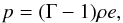 (20)where Γ = 5 / 3 for monoatomic
gas and Γ = 7 /
5 for diatomic gas (see Eqs. (18) and (19)).
(20)where Γ = 5 / 3 for monoatomic
gas and Γ = 7 /
5 for diatomic gas (see Eqs. (18) and (19)).
2.4. Partially ionized hydrogen gas
Astrophysical fluids and processes are more complex than the simple system of ideal gas described above. For example, the ISM that is largely made of hydrogen and helium is affected by many physical and chemical processes viz., collisional ionization, dissociation, shocks, radiation, etc. In such a scenario, an heuristic approach that models the ISM as an monoatomic ideal gas with constant Γ = 5 / 3 will only be approximate and fail to account for the feedback of the above processes on the thermal properties of the gas and thereby also on its inter-linked dynamics.
Consider the simplest case of a partially ionized gas of pure hydrogen (in atomic form).
The thermodynamics of such a system is different from that of a completely ionized (or
completely neutral) gas as the number of free particles can change and an additional
energy contribution is required during the process of ionization. The internal energy
density is therefore given by (Clayton 1984)
 (21)In addition to
the standard form of translational energy, contribution from ionization potential,
χH, is included in Eq. (21). Here, nHII is the
number density of ionized hydrogens and the total number density of free particles,
n =
nH + 2nHII,
is the sum of number densities of neutral hydrogens and twice that of nHII due to
charge neutrality.
(21)In addition to
the standard form of translational energy, contribution from ionization potential,
χH, is included in Eq. (21). Here, nHII is the
number density of ionized hydrogens and the total number density of free particles,
n =
nH + 2nHII,
is the sum of number densities of neutral hydrogens and twice that of nHII due to
charge neutrality.
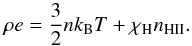
In regions of dense stellar interior, one can assume LTE. For such a system, the fractions of ionized hydrogen becomes non-linearly dependent on temperature and density of the gas through the Saha equation. As a result, internal energy, specific heats and the adiabatic index Γ will depend on the ionization fraction. For example, the adiabatic index Γ will smoothly change from its monoatomic value of 5 / 3 to 1.13 typical of a hydrogen gas with an ionization fraction of 50% at T = 104 K (Clayton 1984). Such a significant change in Γ occurs because part of the energy input becomes available to ionization rather than increasing the temperature of the gas. Therefore, using a constant value of Γ for such dense stellar interiors will considerably overestimate the temperature of the gas.
2.5. Hydrogen/helium gas mixture
 |
Fig. 1 Variation of mean molecular weight μ, internal energy density of the gas (ρe)gas and first adiabatic index Γ1 with temperature. The different colored curves represent four values of fixed density in g cm-3, viz., 10-4 (red), 10-8 (green), 10-12 (blue) and 10-16 (black). The values of (ρe)gas and Γ1 are obtained at equilibrium between ortho and para hydrogen. |
In recent years, studies related to planet formation in accretion disks have started to incorporate EoS that can account for contributions from dissociation of molecular hydrogen, ionization of atomic hydrogen and helium and radiation (e.g., Boley et al. 2007; D’Angelo & Bodenheimer 2013) under an assumption of LTE. In this paper, we have implemented such an EoS both in the presence of LTE1 and with explicit non-equilibrium cooling. For all future references to this EoS, we will use H/He EoS.
In LTE, processes like ionization-recombination and dissociation-bond formation for
hydrogen are given by 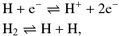 (22)respectively.
Following D’Angelo & Bodenheimer (2013), we
define the degree of dissociation y and degree of ionization x as
(22)respectively.
Following D’Angelo & Bodenheimer (2013), we
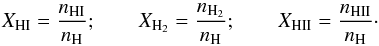
define the degree of dissociation y and degree of ionization x as 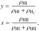 (23)where,
ρHI is the density of atomic hydrogen,
ρH2 the density of molecular
hydrogen and ρHII the density of ionized hydrogen. In
the limit of LTE, one assumes that the level populations due to ionization (and
dissociation) processes follow Boltzmann excitation formula and that the ejected free
electrons thermalize to attain a Maxwell-Boltzmann velocity distribution corresponding to
single gas temperature. This is generally true in regions of high density like that of the
solar interior. In such cases, the degree of ionization using Saha equations is given as
follows,
(23)where,
ρHI is the density of atomic hydrogen,
ρH2 the density of molecular
hydrogen and ρHII the density of ionized hydrogen. In
the limit of LTE, one assumes that the level populations due to ionization (and
dissociation) processes follow Boltzmann excitation formula and that the ejected free
electrons thermalize to attain a Maxwell-Boltzmann velocity distribution corresponding to
single gas temperature. This is generally true in regions of high density like that of the
solar interior. In such cases, the degree of ionization using Saha equations is given as
follows, 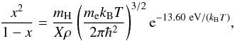 (24)and also degree of
dissociation, y can be obtained in a similar manner (Black & Bodenheimer 1975),
(24)and also degree of
dissociation, y can be obtained in a similar manner (Black & Bodenheimer 1975), 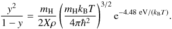 (25)The gas is
essentially a mixture of hydrogen in all forms (atoms, ions & molecules) with a
mass fraction of X, helium with a mass fraction of Y and negligible fraction
of metals. For such a composition the total density of gas is defined as ρ =
nμmH, where the mean
molecular weight μ can be expressed as (e.g., Black & Bodenheimer 1975)
(25)The gas is
essentially a mixture of hydrogen in all forms (atoms, ions & molecules) with a
mass fraction of X, helium with a mass fraction of Y and negligible fraction
of metals. For such a composition the total density of gas is defined as ρ =
nμmH, where the mean
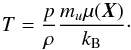
molecular weight μ can be expressed as (e.g., Black & Bodenheimer 1975) ![Mathematical equation: \begin{equation} \label{eq:11} \frac{\mu}{4}= \left[2\textit{X} (1 + y + 2xy) + \textit{Y}\right]^{-1}. \end{equation}](/articles/aa/full_html/2015/08/aa26247-15/aa26247-15-eq104.png) (26)Such a gas mixture is
further assumed to be thermally ideal so that pressure and temperature are related by
p =
ρkBT/
(μmH).
(26)Such a gas mixture is
further assumed to be thermally ideal so that pressure and temperature are related by
p =
ρkBT/
(μmH).
The most crucial part is to express a caloric EoS that can account for contributions from
various degrees of freedom and processes like ionization and dissociation. Thus, the gas
internal energy density (ρe)gas for the mixture is given by
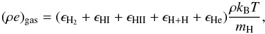 (27)where each term
in parenthesis is dimensionless and can be obtained from an appropriate partition function
and Eq. (18). Table 1 summarizes the different contribution to the gas internal energy.
(27)where each term
in parenthesis is dimensionless and can be obtained from an appropriate partition function
and Eq. (18). Table 1 summarizes the different contribution to the gas internal energy.
In the case of molecular hydrogen, ϵH2, terms that correspond to vibrational and rotational degree of freedom are also considered. These terms are evaluated using the partition function of vibration ζv and rotation ζr that have explicit and a non-linear dependence on temperature. Additionally, the rotational partition function also takes into account the para/ortho H2 spin states (Boley et al. 2007). Thus, the total gas internal energy density has a non-linear dependence on the temperature T and density through x and y (see Eqs. (24) and (25)).
The left and middle panels of Fig. 1 show the variation of μ(ρ,T) (Eq. (26)) and gas internal energy in ergs with temperature, T, for four values of density in g cm-3 respectively. The values of μ are bounded between the upper value ~2.3, corresponding to a fully molecular medium at low temperatures and a lower value ~0.6 at high temperatures representing a fully ionized medium. The transition between these bounds is smooth at large densities ρ = 10-4 g cm-3 while it forms an intermediate plateau at T ~ 103 K at low density values (black curve). The first transition occurs in the temperature range where molecules begin to dissociate to form atomic hydrogen. A second transition takes place where atomic hydrogen becomes ionized. The same transitions can be observed in the profile of internal energy. From a physical point of view they indicate that the energy at these temperatures becomes available to dissociate or ionize the gas rather than heating the gas so that temperature remains approximately constant. Away from these transition regions, the dependence of (ρe)gas(mH/ρ) is linear and increases monotonically with the gas temperature. The last panel of the same figure shows the variation of first adiabatic exponent, Γ1 with temperature. At low temperatures, the gas behaves as a monoatomic ideal gas undergoing adiabatic process with Γ1 = 5 / 3. This is also true at very large temperatures where the gas contains ions and electrons. From the previous considerations, we see a sharp decrease in Γ1 from its maximum value of 5 / 3 to values around unity (corresponding to an isothermal limit) for a low-density plasma (black curve). On the other hand, a single dip at T> 104 K is seen at larger densities (red curve).
In addition to the study of planet formation in accretion disks, the H–He EoS is an important ingredient in the physics of proto-stellar formation from collapse of dense molecular cores. Radiation hydrodynamics simulations (Masunaga et al. 1998; Masunaga & Inutsuka 2000) have put forth detailed understanding of thermodynamics in presence of gravitational collapse. At the onset of collapse, compressional heating in the dense (ρ ~ 104 − 5 g cm-3) and cold (T ~ 10 K) core increases the central temperature up to T ~ 100 K adiabatically. As the temperature increases further, rotational states of H2 are excited and the system evolves with an effective adiabatic index of 7/5 with the ensuing formation of a pressure-supported first core. A further increase in temperature beyond 103 K results in dissociation of H2 which acts as an efficient cooling mechanism leading to a second collapse.
However, not all astrophysical problems can be treated in LTE limit. A classical case is that of a jet, where the recombination time scales are comparable to that of dynamical time. In such a scenario, LTE assumptions become invalid and a non-equilibrium approach has to be adopted as described in the following section.
2.6. Non-equilibrium hydrogen chemistry
Astrophysical flows in HII regions, supernova remnants, star forming regions are some
classical examples where optically thin cooling time scales are comparable to the
dynamical time. In such environments, ionization and dissociation fractions are far from
LTE and their estimation based on Saha fractions can give large errors. In such cases, the
number density of various species is more accurately determined by solving the chemical
rate equations, 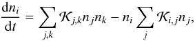 (28)where n is the number density,
 is the rate of formation of ith specie from all j and k species while
 is the rate of destruction of the ith specie due to all j species.
In addition, proper treatment should be carried out to evolve the internal energy to
account for losses due to optically thin radiation, 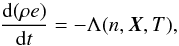 (29)where
Λ(n,X,T)
is the optically thin radiative loss term. Radiative losses imply that the emitted photons
due to different physical processes (e.g., ionization, metal line cooling) freely stream
(without diffusion) away from the region where they are produced and eventually escape
into the surroundings resulting into an effective decrease in total gas internal energy.
(29)where
Λ(n,X,T)
is the optically thin radiative loss term. Radiative losses imply that the emitted photons
due to different physical processes (e.g., ionization, metal line cooling) freely stream
(without diffusion) away from the region where they are produced and eventually escape
into the surroundings resulting into an effective decrease in total gas internal energy.
Summary of the chemistry reaction set. T is the temperature in Kelvin, TeV is the temperature in electron-volts, T5 = T/ 1 × 10⁵ and T2 = T/100.
In presence of cooling, the gas internal energy, (ρe)gas, will be
different from that defined by Eq. (27).
Indeed, only contributions due to translational and internal degrees of freedom (from H,
He and H2) should
be included. Conversely, terms corresponding to the emission of photons (e.g., ionization,
dissociation, roto-vibrational cooling of H2 molecule) are correctly accounted for by the right
hand side of Eq. (29) in the
Λ term. Therefore Eq. (27) now becomes  (30)where,
expressions for each of the internal energy components are given in Table 1. A similar contribution to gas internal energy (see.
Eq. (29)) from internal degrees of freedom
in presence of radiative losses has also been applied to study the role of molecular
hydrogen in primordial star formation (e.g., Palla et al.
1983; Omukai & Nishi 1998).
(30)where,
expressions for each of the internal energy components are given in Table 1. A similar contribution to gas internal energy (see.
Eq. (29)) from internal degrees of freedom
in presence of radiative losses has also been applied to study the role of molecular
hydrogen in primordial star formation (e.g., Palla et al.
1983; Omukai & Nishi 1998).
For the present purpose, we focus only on the chemical evolution of atomic and molecular
hydrogen. In particular, the total hydrogen number density nH includes
contributions from atomic and molecular hydrogen i.e., nH =
nHI +
2nH2 +
nHII. Contributions to the electrons
density ne come from ionized hydrogen
(nHII) and from a small but fixed fraction
of metals (Z ~
10-4). In addition to hydrogen, we also consider helium to
be present with a fixed mass fraction of 0.027. The mass density ρ =
μntotmp
is a conserved quantity whereas the total number of particle per unit volume
(ntot =
nH + nHe +
ne) is not as it may change owing to
ionization, recombination and dissociation processes. The chemical evolution of molecular,
atomic and ionized hydrogen is governed by the equations listed in Table 2. The code tracks the formation and destruction of
these three species based on the temperature-dependent reaction rates specified and
updates the corresponding number fractions,
 (31)In dilute regions
such as the solar corona, Eq. (28) can be
simplified by setting dni/
dt = 0 as the time scales are such that a balance is
always maintained between collisional ionization and radiative recombination. This
condition is known as coronal equilibrium or collisional ionization equilibrium (CIE) and
it differs from LTE in two aspects: i) it is only valid in dilute plasma – unlike the LTE
where high-density environments are required – and ii) the ionization fraction are
estimated using Eq. (28) in steady state
and not with Saha fractions. The top panel of Fig. 2
shows the concentration fractions as functions of temperature obtained by solving the
steady state version of Eq. (28). The
dissociation and ionization of molecular and atomic hydrogen, respectively, are clearly
evident at the temperatures of T ~ 3 × 10³ K and T ~ 104 K. Such
equilibrium values can be used to initialize fractions in numerical computations.
(31)In dilute regions
such as the solar corona, Eq. (28) can be
simplified by setting dni/
dt = 0 as the time scales are such that a balance is
always maintained between collisional ionization and radiative recombination. This
condition is known as coronal equilibrium or collisional ionization equilibrium (CIE) and
it differs from LTE in two aspects: i) it is only valid in dilute plasma – unlike the LTE
where high-density environments are required – and ii) the ionization fraction are
estimated using Eq. (28) in steady state
and not with Saha fractions. The top panel of Fig. 2
shows the concentration fractions as functions of temperature obtained by solving the
steady state version of Eq. (28). The
dissociation and ionization of molecular and atomic hydrogen, respectively, are clearly
evident at the temperatures of T ~ 3 × 10³ K and T ~ 104 K. Such
equilibrium values can be used to initialize fractions in numerical computations.
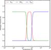 |
Fig. 2 Different hydrogen fractions (XHI: atomic red, XH2: molecular green and XHII: ionized blue) obtained at equilibrium for different temperatures. We note that the total sum of fractions, i.e., XHI + 2XH2 + XHII is conserved. |
The radiative losses implemented in our model can be written as  (32)where,
ΛCI and
ΛRR are losses
due to collisional ionization and radiative recombination, respectively (Teşileanu et al. 2008). The remaining terms,
Λrotvib,
ΛH2diss and
Λgrain are
associated with molecular hydrogen and represent losses due to rotational-vibrational
cooling, dissociation and gas-grain processes (Smith
& Rosen 2003).
(32)where,
ΛCI and
ΛRR are losses
due to collisional ionization and radiative recombination, respectively (Teşileanu et al. 2008). The remaining terms,
Λrotvib,
ΛH2diss and
Λgrain are
associated with molecular hydrogen and represent losses due to rotational-vibrational
cooling, dissociation and gas-grain processes (Smith
& Rosen 2003).
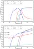 |
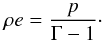
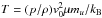
Fig. 3 Top panel: variation with temperature of cooling function arising from different processes obtained using equilibrium values of hydrogen fractions (that vary with temperature as shown in Fig. 2) in units of erg cm3 s-1 for a total number density n0 = 105 cm-3. Bottom panel: different components of radiative cooling functions with same initial number density, n0 but for fixed values of concentration fractions (mentioned in the figure). In both panels, the sum of all the components is drawn with a black dashed line to obtain the value of Λ in erg cm3 s-1 following Eq. (32). |
The dependence of the cooling function,  , for
n0 =
105 cm-3 is shown in the top and bottom panels of Fig. 3. In the top panel, cooling functions are plotted using
concentrations values obtained under CIE conditions while the plots in the bottom panel
corresponds to fixed concentrations obtained for T = 4500 K. For
temperatures T< 104 K, the
total cooling function with equilibrium values of hydrogen fractions (black dashed curve)
is dominated by the contribution of roto-vibrational cooling of molecular hydrogen (blue
line). Molecular cooling due to dissociation (green curve) and gas-grain processes (red
curve) have little impact on the total cooling function. For temperatures T>
104 K, most of the hydrogen molecules have dissociated into
atoms (see Fig. 2) and the total cooling curve in
Fig. 3 is governed by atomic processes like radiative
recombination (cyan line) and collisional ionization (magenta line).
, for
n0 =
105 cm-3 is shown in the top and bottom panels of Fig. 3. In the top panel, cooling functions are plotted using
concentrations values obtained under CIE conditions while the plots in the bottom panel
corresponds to fixed concentrations obtained for T = 4500 K. For
temperatures T< 104 K, the
total cooling function with equilibrium values of hydrogen fractions (black dashed curve)
is dominated by the contribution of roto-vibrational cooling of molecular hydrogen (blue
line). Molecular cooling due to dissociation (green curve) and gas-grain processes (red
curve) have little impact on the total cooling function. For temperatures T>
104 K, most of the hydrogen molecules have dissociated into
atoms (see Fig. 2) and the total cooling curve in
Fig. 3 is governed by atomic processes like radiative
recombination (cyan line) and collisional ionization (magenta line).
The total cooling curve in the bottom panel of Fig. 3 with fixed values of hydrogen fractions differs substantially from the panel above. It is dominated by gas grain processes (red line) for T< 100 K. For temperatures between 100 K and 104 K, molecular cooling due to rotational and vibrational processes (blue line) plays a vital role. Even at large temperatures, T> 104 K, the total cooling curve has major contribution from molecular dissociation (green line), for the chosen fixed fraction of molecules. The contribution of collisional ionization (magenta line) also becomes important at these temperatures. However, the cooling due to radiative recombination remain negligible for all temperature values due to extremely small and fixed fraction of electrons, XHII.
Equations being solved when converting from pressure to internal energy (p → ρe) or vice versa (ρe → p).
3. Numerical implementation
In a Godunov-type scheme the MHD Eqs. (1)−(5) are discretized using a flux-conserving form
where the basic building block is ![Mathematical equation: \begin{equation} \label{eq:conservative_update} \vec{U}^{n+1}_{\vec{i}} = \vec{U}^n_{\vec{i}} - \frac{\Delta t^n}{\Delta{\cal V}_{\vec{i}}} \sum_d\Big[\left(A_d\vec{F}_d\right)_{\vec{i}+\HALF\hat{\vec{e}}_d} -\left(A_d\vec{F}_d\right)_{\vec{i}-\HALF\hat{\vec{e}}_d}\Big] + \vec{S}_{\vec{i}}, \end{equation}](/articles/aa/full_html/2015/08/aa26247-15/aa26247-15-eq205.png) (33)where U =
(ρ,ρv,B,E,ρXk)
is our vector of conservative variables, Δtn is the time step and
Si
is a source term. Here we employ an orthogonal system of coordinates with unit vectors
(33)where U =
(ρ,ρv,B,E,ρXk)
is our vector of conservative variables, Δtn is the time step and
Si
is a source term. Here we employ an orthogonal system of coordinates with unit vectors
 (here d =
1,2,3 or simply x,y,z) where Ad is the area element in
the d
direction, Fd is the
flux computed with a Riemann solver,
(here d =
1,2,3 or simply x,y,z) where Ad is the area element in
the d
direction, Fd is the
flux computed with a Riemann solver,  is the cell volume while i = (i,j,k) is the
position of the computational zone in the domain. We remind the reader to Mignone et al. (2007), Teşileanu et al. (2008) and Mignone et al.
(2012) for more details. Here we focus only on those aspects that crucially depend
on the choice of the equation of state, namely: i) the computation of the flux via a Riemann
solver and ii) the conversion between internal energy and pressure.
is the cell volume while i = (i,j,k) is the
position of the computational zone in the domain. We remind the reader to Mignone et al. (2007), Teşileanu et al. (2008) and Mignone et al.
(2012) for more details. Here we focus only on those aspects that crucially depend
on the choice of the equation of state, namely: i) the computation of the flux via a Riemann
solver and ii) the conversion between internal energy and pressure.
3.1. Solution of the Riemann problem
The Riemann problem is an initial value problem describing the decay of a discontinuity separating two constant states. As time evolves, the discontinuity breaks into a set of non-interacting elementary waves whose properties are determined by connecting, in a self-consistent way, the initial left and right states through wave-curves. For a convex EoS, as defined in Sect. 2.2, the solution to the Riemann problem in hydrodynamics consists of a left-facing shock or rarefaction wave, a contact discontinuity and a right-facing wave (again either a shock or a rarefaction). No compound wave can be formed in the solution. In MHD the solution may involve up to 7 modes: a pair of fast magneto-sonic waves, a pair of Alfvén waves (or rotational modes) and a pair of slow waves and a contact (or tangential) discontinuity in the middle. Although exact solutions to the Riemann problem are possible, the computational overhead is largely reduced by using approximate solvers based on different levels of simplification.
A first class of solvers heavily relies on characteristic (Jacobian) decomposition or computation of Riemann invariants which is strictly connected with the underlying form of the conservation law. Typical examples are linearized (Roe-type), flux-splitting or two-shock approximate solvers, see the book by Toro (2009). Solvers belonging to this class require considerable changes when new physical ingredients (such as a different EoS) are introduced. In the case of real gases, for instance, extensions have been presented by Colella & Glaz (1985), Glaister (1988b,a), Buffard et al. (2000) (in the case of the Euler or Navier-Stokes equations) while generalization to the MHD case have been presented in Dedner & Wesenberg (2001). In Fedkiw et al. (1997) a Roe-type Riemann solver for the solution of thermally ideal, chemically reacting gases has been presented in the context of the multi-species Navier-Stokes equations.
A second class of solvers employs only minimal information (typically approximate expressions for the wave speeds) and it is based on an application of the integral form of the conservation laws which gives a closed-form approximate expression for the fluxes. Typical examples are the Lax-Friedrichs-Rusanov (Tóth & Odstrčil 1996), Harten-Lax-van Leer (HLL, see Harten et al. 1983) solver and their extensions such as HLLC (Toro et al. 1994; Gurski 2004; Li 2005) and HLLD (Miyoshi & Kusano 2005). Solvers belonging to this class can accomodate new changes with minimal efforts by simply changing the definition of the sound speed and, for this reason, will be our preferred method of choice. Incidentally, we also note that, since only an approximate expression for the eigenvalue is needed and Γ1 ≤ 5 / 3, employing Eq. (9) with Γ1 = 5 / 3 provides an upper bound to the actual expression with a only a slight loss of accuracy.
3.2. Conversion between internal energy and pressure
The computation of the right hand side of Eq. (33) is normally carried out using primitive variables customarily defined as V = (ρ,v,B,p). The conversion between U and V requires obtaining pressure from total energy density and vice versa. While internal energy density is readily obtained from Eq. (6), the conversion p → ρe and its inverse ρe → p strictly depends on the choice of the caloric equation of state.
For the constant-Γ EoS, these
transformations take a small fraction of the computational time as the relation between
internal energy and pressure is straightforward and given by
 (34)We also note that the
temperature does not explicitly appears in the previous definition.
(34)We also note that the
temperature does not explicitly appears in the previous definition.
The situation is different, however, for a more general EoS where a closed-form
expression between pressure and internal energy may not be easy to obtain. From the
considerations given in the previous sections, in fact, we can write the thermal and
caloric equations of state as 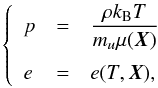 (35)where
X may be an independent variable or, in
equilibrium conditions, a function of temperature and density. The explicit dependence on
the temperature introduces two additional intermediate steps, namely:
(35)where
X may be an independent variable or, in
equilibrium conditions, a function of temperature and density. The explicit dependence on
the temperature introduces two additional intermediate steps, namely:
-
1.
During the conversion p → ρe one first needs to compute T from the thermal EoS (first of Eq. (35)):
 (36)Under
non-equilibrium conditions, μ =
μ(X) is a known
function of the gas composition and Eq. (36) can be solved directly. Under LTE or CIE, on the other hand,
X =
X(T,ρ) is a
function of density and temperature and Eq. (36) becomes a non-linear equation in the temperature variable.
(36)Under
non-equilibrium conditions, μ =
μ(X) is a known
function of the gas composition and Eq. (36) can be solved directly. Under LTE or CIE, on the other hand,
X =
X(T,ρ) is a
function of density and temperature and Eq. (36) becomes a non-linear equation in the temperature variable.
-
2.
During the inverse transformation (ρe → p), one must first solve for the temperature by inverting
 (37)where, under
equilibrium assumptions, the chemical composition is a function of temperature and
density, i.e., X =
X(T,ρ).
(37)where, under
equilibrium assumptions, the chemical composition is a function of temperature and
density, i.e., X =
X(T,ρ).
Table 3 summarizes the relevant equations to be solved.
In order to cope with the numerical inversion of Eqs. (36) and (37) we have considered and implemented two different solution strategies that we describe in the following sections.
3.2.1. Conversion using root finders
In this approach we employ the exact analytical expressions (36), (37) to compute pressure and internal energy as functions of temperature or vice versa. For the caloric EoS, numerical inversion using a root-finder algorithm is required to obtain T from ρe(T,X) or ρe(T,ρ) as they are both non-linear functions of the temperature. Additionally, under LTE or CIE, the thermal EoS must also be inverted numerically to obtain temperature since the mean molecular weight introduces non-linearity. These cases are marked with a * in Table 3.
The root-finder approach results in increased computational cost inasmuch the internal energy is an expensive function to evaluate. Among different root-solvers not requiring the knowledge of the derivative, we have found Brent’s or Ridders’ methods to be practical and efficient root-finding algorithms.
3.2.2. Conversion using tables
A second and more efficient strategy can be used when the internal energy is a function
of temperature and density alone (which is typically the case under equilibrium
conditions, CIE or LTE) and it consists of employing pre-computed tables of pressure and
internal energy, e.g.,  (38)where
i =
0,...,Nc
− 1 and j
=
0,...,Nr
− 1 are the table indices. For convenience, the tables are
constructed using equally-spaced node values in log T and log ρ so that
log Ti/T0
= iΔlog T and log ρj/ρ0
= jΔlog ρ where ρ0 and
T0 are the lowest density and
temperature values in the table. Following this approach, Eqs. (36), (37) and their inverses are replaced by direct or reverse lookup
table operations. We point out that, in order to be invertible, tables must be obtained
from monotone functions of their arguments and this is always verified for the EoS of
interest.
(38)where
i =
0,...,Nc
− 1 and j
=
0,...,Nr
− 1 are the table indices. For convenience, the tables are
constructed using equally-spaced node values in log T and log ρ so that
log Ti/T0
= iΔlog T and log ρj/ρ0
= jΔlog ρ where ρ0 and
T0 are the lowest density and
temperature values in the table. Following this approach, Eqs. (36), (37) and their inverses are replaced by direct or reverse lookup
table operations. We point out that, in order to be invertible, tables must be obtained
from monotone functions of their arguments and this is always verified for the EoS of
interest.
When T and
ρ are
known, for instance, pressure and internal energy are obtained by using lookup table
followed by 2D interpolation between adjacent node values. Thus we first locate the
table indices i and j by a simple division,  (39)where
T and
ρ are the
input values at which interpolation is desired. Internal energy (and similarly pressure)
is then computed as
(39)where
T and
ρ are the
input values at which interpolation is desired. Internal energy (and similarly pressure)
is then computed as  (40)where
x = (T −
Ti) /
(Ti + 1 −
Ti) and
y = (ρ −
ρj) /
(ρj + 1 −
ρj) are normalized coordinates between
adjacent nodes while
(40)where
x = (T −
Ti) /
(Ti + 1 −
Ti) and
y = (ρ −
ρj) /
(ρj + 1 −
ρj) are normalized coordinates between
adjacent nodes while  is an interpolating spline, see Sect. 3.2.3.
Conversely, when ρe and ρ are known, Eq. (40) must be inverted to obtain T. To this end, we first
locate the index j using the second of (39) with ρ given. In order to find
the column index i, we first construct the intermediate 1D array
qi = { ρe }
i,j(1 − y) + { ρe }
i,j + 1y with
j fixed
from the previous search whereas i =
0,...,Nc.
A binary search is then performed on qi to obtain
i and Eq.
(40) can be inverted to obtain
x.
Temperature is finally obtained as T = Ti +
x(Ti + 1 −
Ti). The inversion
depends on the choice of the interpolating function
and it is discussed in more detail in the next section.
The tabulated approach has found to be faster than the general root finder method giving considerable speedups, up to a factor of 4 for certain problems.
3.2.3. Choice of the interpolant
For linear interpolation, we simply use  (41)in Eq. (40) so that internal energy and pressure
become bilinear functions of temperature and density. When ρe is given, on the other
hand, the inverse function is required to compute temperature and one needs to solve Eq.
(40) with
(41)in Eq. (40) so that internal energy and pressure
become bilinear functions of temperature and density. When ρe is given, on the other
hand, the inverse function is required to compute temperature and one needs to solve Eq.
(40) with
 given by Eq. (41) to obtain
x. Since
the resulting equation is linear in x one readily finds
given by Eq. (41) to obtain
x. Since
the resulting equation is linear in x one readily finds  (42)where
f =
ρe, fi,j = { ρe }
i,j or f = p,
fi,j = { p }
i,j. Despite its simplicity, however,
bilinear interpolation may generate thermodynamically inconsistent results since the
positivity of the fundamental derivative (Eq. (16)) can be violated at node points in the table where derivatives are not
continuous. This generates composite waves in the solution due to a loss of convexity of
the caloric EoS as discussed in Sect. 2.2. Indeed,
we have verified that this pathology worsen as the number of points in the temperature
grid is reduced. An illustration of the problem is reported in Appendix B.
(42)where
f =
ρe, fi,j = { ρe }
i,j or f = p,
fi,j = { p }
i,j. Despite its simplicity, however,
bilinear interpolation may generate thermodynamically inconsistent results since the
positivity of the fundamental derivative (Eq. (16)) can be violated at node points in the table where derivatives are not
continuous. This generates composite waves in the solution due to a loss of convexity of
the caloric EoS as discussed in Sect. 2.2. Indeed,
we have verified that this pathology worsen as the number of points in the temperature
grid is reduced. An illustration of the problem is reported in Appendix B.
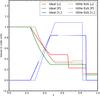 |
Fig. 4 Variation of density ρ (red), pressure P (green), and velocity vx (blue) along the x-axis (in code units) for a standard Sod Tube test (without explicit cooling) at time τ = 0.2. The values obtained using an ideal EoS are shown as solid lines while that obtained using a GammaLaw EoS are shown as dashed lines. |
To overcome this limitation, we have also implemented a cubic spline when interpolating
along the temperature grid so that  (43)where
the coefficients a,b,c and d are computed by
ensuring that the cubic is strictly monotonic in the interval [
Ti,Ti
+ 1 ] see Appendix C.
The inverse function requires finding the root of a cubic equation on a specific
interval and, since the spline is monotone by construction, only one root is always
guaranteed to exist. Thus combining Eq. (43) with Eq. (40) one obtains
the following equation,
(43)where
the coefficients a,b,c and d are computed by
ensuring that the cubic is strictly monotonic in the interval [
Ti,Ti
+ 1 ] see Appendix C.
The inverse function requires finding the root of a cubic equation on a specific
interval and, since the spline is monotone by construction, only one root is always
guaranteed to exist. Thus combining Eq. (43) with Eq. (40) one obtains
the following equation,  (44)where
 and similarly for the
remaining coefficients. Although standard analytical solvers (e.g., Cardano) may be
used, we have found root-finder methods to be more robust, accurate and computational
efficient for the purpose. Starting from an initial guess given by Eq. (42), one can either use Newton-Raphson
method to achieve quadratic convergence,
and similarly for the
remaining coefficients. Although standard analytical solvers (e.g., Cardano) may be
used, we have found root-finder methods to be more robust, accurate and computational
efficient for the purpose. Starting from an initial guess given by Eq. (42), one can either use Newton-Raphson
method to achieve quadratic convergence,
![Mathematical equation: \begin{eqnarray} x^{[k+1]} = x^{[k]} - \frac{h(x^{[k]})}{h'(x^{[k]})} , \end{eqnarray}](/articles/aa/full_html/2015/08/aa26247-15/aa26247-15-eq264.png) (45)or
Halley’s method which gives cubic convergence,
(45)or
Halley’s method which gives cubic convergence,
![Mathematical equation: \begin{equation} x^{[k+1]} = x^{[k]} - \frac{2h(x^{[k]})h'(x^{[k]})}{2[h'(x^{[k]})]^2 - h(x^{[k]})h''(x^{[k]})}\cdot \end{equation}](/articles/aa/full_html/2015/08/aa26247-15/aa26247-15-eq265.png) (46)We have found that both
methods hardly ever require more than three iterations to achieve an absolute accuracy
of 10-11.
(46)We have found that both
methods hardly ever require more than three iterations to achieve an absolute accuracy
of 10-11.
4. Numerical benchmarks
The computational framework presented in this work has been implemented in the PLUTO code (Mignone et al. 2007, 2012). Selected numerical benchmarks are now presented with the aim of investigating the influence of the EoS on problems of astrophysical relevance as well as comparing the computational efficiency of the proposed numerical approaches.
4.1. Sod shock tube
In our first test, we consider the standard Sod shock tube on the unit interval
x ∈ [ 0,1
] with a uniform grid resolution Δx = 10-3. The
initial setup consists of two fluids initially separated by a discontinuity located at
x = 0.5.
Density and pressure in the two regions are given by (ρ,p) =
(1, 1) for x<
0.5 and (ρ,p) = (1 / 8, 1
/ 10) for x> 0.5 while the velocity
is zero everywhere. We choose our physical units in such a way that the reference velocity
is v0 = 5.25 ×
105 km s-1 so that the temperature, in Kelvin, is expressed by
 . With this
choice, the temperatures in the left and right regions become TL ~ 3852 K and
TR ~
3345 K. The final solution at t = 0.2 is shown in Fig.
4 for the adiabatic run (i.e., without explicit
cooling). The test is repeated also by including thermal losses and the solution is
plotted in Fig. 5.
. With this
choice, the temperatures in the left and right regions become TL ~ 3852 K and
TR ~
3345 K. The final solution at t = 0.2 is shown in Fig.
4 for the adiabatic run (i.e., without explicit
cooling). The test is repeated also by including thermal losses and the solution is
plotted in Fig. 5.
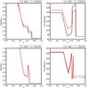 |
Fig. 5 Variation of density (left panels) and temperature (right panels) at the final stage of Sod shock tube test for cases which have included explicit cooling. The black line represent values obtained from ideal EoS, while those obtained using H/He EoS are shown in red. The top and bottom panels differ in the value of their initial temperature on either sides of the interface at x = 0.5. |
4.1.1. Adiabatic shock tube
Figure 4 compares the spatial variation of density, pressure and velocity for an ideal EoS (solid lines) with that of a H/He EoS dashed lines) without explicit cooling. The solution comprises, from left ro right, a rarefaction wave, contact discontinuity and a right-going shock. Pressure and velocity are always continuous across the contact wave. In the case of the gas with H/He EoS we obtain a larger compression ratio (≈ 2.8 compared to ≈ 1.84 of the ideal gas) and the shock propagates slightly slower. Similarly the tail and the head of the rarefaction wave both propagate at a smaller speed and this is due to a reduced value of the sound speed. The density jump across the contact wave is largely reduced with the H/He EoS.
It is important to understand that in the case of an ideal EoS, only translation degrees of freedom contribute to the internal energy which is a linear function of the temperature, see Eq. (18). In the case of the H/He EoS, however, the internal energy also takes contributions from additional degrees of freedom due to rotations and vibrations of di-atomic molecules (like H2 at low temperatures). These will not correspond to an increase in temperature. Therefore, across a shock wave, the upstream kinetic energy will become available to the system not only to raise the temperature, but also to populate the vibrational and rotational levels of the molecules (at lower temperatures), dissociate molecules and eventually ionize atoms (at larger temperatures). Hence we expect the overall increase in temperature to be smaller in the case of H/He EoS than that of an ideal EoS.
Finally we point out that while the employment of an ideal EoS gives a scale-free and self-similar solution to the Sod shock tube, the same argument does not hold for the H/He EoS which implicitly contains temperature scales corresponding to the above mentioned transitions.
4.1.2. Radiative shock tube
We have repeated the Sod shock tube including the explicit non-equilibrium cooling described in Sect. 2.6. We consider two initial conditions corresponding to different values of temperature. In the first case the temperature of the left and right states is set to TL = 400 K and TR = 200 K, respectively. The second case corresponds to hotter gas, TL = 4500 K and TR = 3500 K. Molecular and atomic hydrogen fraction are initially set to their equilibrium values at the local temperature (see Fig. 2).
Figure 5 shows the density and temperature (T/μ, μ being the mean molecular weight). In all panels, solution obtained using an ideal EoS is shown as a black line, whereas that obtained using H/He EoS with a red line.
For smaller initial temperatures (top panels), the density and temperature jumps differ by a modest factor (≈ 20%) and the positions of the waves is essentially the same. The differences are not as large as in the adiabatic case since the H/He EoS, now given by Eq. (30), only includes terms related to the internal degrees of freedom, see Sect. 2.6. Terms related to dissociation and ionization correspond to energy losses and are thus accounted for by the cooling function Λ. These terms are common to both EoS. The presence of molecules at low temperature gives a considerable contribution to the internal energy budget. Hence part of the thermal energy available at the shock serves in populating the internal molecular degrees of freedom rather than raising the temperature. As a consequence, radiative losses are slightly less efficient for the H/He EoS.
For larger initial temperatures (bottom panels) differences are negligible and this behavior is due to a reduced cooling length scale. Indeed, in presence of a shock wave, the gas behind the front undergoes a rapid increase in the temperature while the level populations of H2 do not occur instantaneously (Flower et al. 2003). Since the cooling time scale is shorter than the average time scale over which level population takes place, internal energy changes are dominated by radiative losses. Since the cooling function Λ is the same for both EoS the final solutions are very similar.
These different test cases elucidates the importance of treating temperature-dependent EoS both when the system is in equilibrium and also when explicit radiative cooling is involved.
4.2. MHD shock tube
Next we consider the collision between two magnetized fluids moving in opposite
directions. The problem is studied on the unit interval x ∈ [ 0,1
] with initial condition given as follows:
 (47)The
fluid on the left has larger inertia than the fluid on the right and it is also more
magnetized. We solve the problem by using linear interpolation on characteristic
variables, the HLLD Riemann solver and an adaptive resolution consisting of a base grid of
128 zones and
7 levels of refinement with
consecutive jump ratios of 2
except for refining level 3
where the grid jump is 4.
(47)The
fluid on the left has larger inertia than the fluid on the right and it is also more
magnetized. We solve the problem by using linear interpolation on characteristic
variables, the HLLD Riemann solver and an adaptive resolution consisting of a base grid of
128 zones and
7 levels of refinement with
consecutive jump ratios of 2
except for refining level 3
where the grid jump is 4.
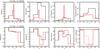 |
Fig. 6 From top left to bottom right: solution at time t = 0.08 of density, pressure, internal energy density (ρe), temperature, X and Y components of velocity, Y component of magnetic field and adiabatic index respectively. In each panel, quantities obtained for ideal EoS are shown in (black) while the red line denotes values obtained using H/He EoS. |
The solution is shown in Fig. 6 at t = 0.08 for the ideal and H/He EoS. In order to carry out a fair comparison, we have chosen the adiabatic index of the ideal EoS to be Γ = 1.447 so that the gas internal energy has the same value for both EoS at t = 0. The wave pattern consists of a pair of outer fast magneto-sonic shocks enclosing two slow magneto-sonic shocks and a contact wave in the middle.
Overall, shocks are stronger and propagate faster for the ideal gas case leading to the formation of a more extended Riemann fan owing to a larger value of the sound speed (Eq. (10)). This is evident from looking at the profiles of the first adiabatic index shown in the bottom right panel of Fig. 6. For the H/He EoS, Γ1 drops to ≈ 1.04 in the shocked regions while it remains constant for the ideal EoS. This effect becomes more pronounced at the two slow shocks which, in the case of H/He gas, propagate to the left at very small velocities forming a very thin shell of compressed material with large internal energy.
In spite of the reduced shock strength, however, the density compression attained at shocks is nearly the same or even larger for the H/He gas. This behavior can be understood by noticing that lower values of the specific heat ratio should support larger density jumps. Indeed, the effective Γ-value, defined as Γeff = p/ (ρe) + 1 (dashed line in the bottom right panel of Fig. 6), becomes smaller with the H/He EoS thus allowing for comparable or larger compression ratios (in density and magnetic field) even if the shock is weaker.
The EoS largely determines how the upstream kinetic energy is being converted into internal energy and heat: for the ideal gas an increase in internal energy corresponds to an increment in pressure and temperature while, in the range of temperature considered here (102 K ≲ T ≲ 104 K), the same does not hold for the gas with H/He EoS. In this case, in fact, the downstream internal energy is employed to excite internal vibrational and rotational levels without a corresponding increase in pressure or temperature.
4.3. Blast wave
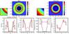 |
Fig. 7 Top panels: comparison of density ρ (in code units) for a hydrodynamic, spherical blast wave at time t = 0.15. Left panel: final shock structure with an ideal EoS. Top right panel: density obtained using the H/He EoS. Alongside each panel a zoomed in view of density around the contact discontinuity is shown. The ideal EoS shows presence of Rayleigh-Taylor instability while its completely absent in case of H/He EoS. Bottom panels from left to right: comparison of 1D cuts at the mid-plane of density ρ, pressure p, temperature (T/μ) and velocity (vx) for ideal EoS (black line) and H/He EoS (red line). |
We now consider a 2D blast wave in Cartesian coordinates on the square domain
−
L0/ 2
<x,y<L0/
2 where L0 = 2.5 × 1015 cm. An
over-dense and over-pressurized region is initialized at the center of the domain
(x = y =
0) inside a circular region of radius r0/L0 =
0.1 where density and pressure are set respectively to ρ/ρa =
10 and p/pa =
20 in units of the corresponding ambient values, ρa =
namH and
 (here we use
na =
105 cm-3 and v0 = 2.5 km s-1). The computation is carried
using adaptive mesh refinement (AMR) using a base grid of 256 × 256 grid zones and 4 levels of refinement (effective resolution
of 40962 zones).
The MUSCL-Hancock with piecewise linear interpolation and the HLLC Riemann solver are
employed.
(here we use
na =
105 cm-3 and v0 = 2.5 km s-1). The computation is carried
using adaptive mesh refinement (AMR) using a base grid of 256 × 256 grid zones and 4 levels of refinement (effective resolution
of 40962 zones).
The MUSCL-Hancock with piecewise linear interpolation and the HLLC Riemann solver are
employed.
The solution features an outermost forward shock wave followed by a contact discontinuity and a reverse shock as shown in the top panel of Fig. 7 at t = 0.15. In analogy with the Sod shock tube problem, we observe that the size of the spherical blast wave is smaller when the H/He EoS is employed although the shock strengths (measured in terms of pressure jumps) are comparable for both EoS. The compression ratio across the forward shock is noticeably larger for the H/He EoS (~ 2.7) than for the ideal EoS (~ 1.7) owing to a reduced value of the equivalent adiabatic index.
An important difference lies in the structure of the contact wave as it can be noticed in the closeups in the bottom panel of Fig. 7. In the ideal EoS case, the density contrast across the contact wave is favorable to the onset of the Rayleigh-Taylor instability while the same structure is stable for the H/He EoS since the density contrast is reversed (heavy fluid in front, light fluid behind). Thus a shell of high-density material is swept between the outermost shock and the contact wave.
From the computational perspective, we have compared the ideal and H/He EoS in terms of speed. Our results show that the average wall clock time per numerical step is 0.05 s with the ideal EoS while we found 0.25 s and 0.9 s for the tabulated and the root finder approaches, respectively, in the case of H/He EoS. As expected the computation with constant Γ are the fastest ones. However, it is interesting to note that pre-computed tabulated values give a speed up of about 4 times than that obtained using the root finder approach, while maintaining essentially the same accuracy in the final solution.
4.4. One-dimensional pulsed molecular jets
As an astrophysical applications, we consider in the next test the propagation of velocity pulsations in a 1D molecular jet model that includes radiative losses. Multi-dimensional extensions of this study will be considered in forthcoming papers.
In order to resolve the thin post-shocked regions we employ adaptive mesh refinement to
enhance resolution in high-temperature and dense regions. The computational domain extends
from z = 0 up
to z = 32 in
units of the jet radius rj ~ 75 AU and it is covered by a base
grid of 256 grid zones. We
employ 10 levels of refinement
yielding an equivalent resolution of 262,144 zones. The domain is initially filled with
a fully molecular (XH2 ≈ 0.5) ambient
representing a young star-forming core at the temperature of Ta = 50 K and
decreasing density so that 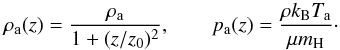 (48)In the previous equation
ρa is the ambient density at
z = 0 while
z0 =
10rj. An over-dense jet (ρj/ρa =
3) is injected from the nozzle at z = 0 with temperature
Tj =
103 K resulting in an over-pressurized jet
(pj/pa ≈
60). The initial hydrogen fractions at the nozzle are estimated based
on equilibrium shown in Fig. 2 while the jet density
is assumed to be ρj
= njmH with
nj =
104 cm-3. The injection velocity has sinusoidal perturbations
of the form vj =
v0 (1 +
0.25sin(2πt/Tp)),
with base velocity v0 = 70 km s-1 and pulsation period
Tp =
40 years.
(48)In the previous equation
ρa is the ambient density at
z = 0 while
z0 =
10rj. An over-dense jet (ρj/ρa =
3) is injected from the nozzle at z = 0 with temperature
Tj =
103 K resulting in an over-pressurized jet
(pj/pa ≈
60). The initial hydrogen fractions at the nozzle are estimated based
on equilibrium shown in Fig. 2 while the jet density
is assumed to be ρj
= njmH with
nj =
104 cm-3. The injection velocity has sinusoidal perturbations
of the form vj =
v0 (1 +
0.25sin(2πt/Tp)),
with base velocity v0 = 70 km s-1 and pulsation period
Tp =
40 years.
As the system evolves, velocity pulsations steepen into a chain of forward/reverse shock pairs, the first of which becomes the strongest one reaching temperatures of T ~ 105 K where hydrogen is quickly ionized. Under these physical conditions the two EoS yields essentially the same results since thermal kinetic motion is characterized only by translational degrees of freedom.
Successive pulses, however, form weaker shocks with temperatures of a few thousand K, see Fig. 8. As the cooling time is much smaller than the dynamical time, the material behind the shocks start to cool radiatively in a very efficient way. Temperature peaks immediately downstream of the forward and reverse shocks and quickly drops afterwards forming extremely thin layers of hot material (see the enlargement in the right panel of Fig. 8). The layer of fluid between the forward/reverse shock pairs becomes nearly isobaric with a high-density pile. We point out that the numerical resolution of such layers is crucial in order to correctly capture the physical processes (such as ionization and radiative losses) taking place on different time scales. The importance of grid resolution has also been addressed by Teşileanu et al. (2009) in the context of time-dependent radiative shocks subject to atomic cooling.
As it has been elucidated in earlier tests, the transformation of upstream kinetic energy into internal energy depends on the EoS considered. While pressure is essentially the same for both EoS, the temperature values reached immediately behind the shocks are larger for the ideal EoS gas than for the H–He EoS because part of the internal energy is employed to dissociate molecules. As a consequence the amount of atomic hydrogen produced during the dissociation process is halved (~ 2.7% for the H–He EoS vs. ~ 5.9% with the ideal EoS).
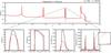 |
Fig. 8 Results from the test studying the propagation of supersonic pulsations in molecular medium. Top panel: comparison of density (in code units) for ideal EoS (black line) and H/He EoS (red line) on a log scale at time t = 192 yr. Bottom panels: comparison of zoomed up quantities for a particular knot marked within the rectangle in the top panel using the same color keys. These quantities from left to right are density ρ, pressure p, HI fraction XHI and temperature T/μ. A zoomed inset of the forward shock obtained from H/He EoS is shown as well with red dots to demonstrate the importance of resolving the shock (see text). |
4.5. Axisymmetric MHD jets
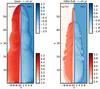 |
Fig. 9 Comparison of logarithmic values both of density, ρ (right half in blues) and temperature in Kelvin (left half in red) for a 2D axisymmetric jet without explicit cooling. The left panel shows the jet structure with an ideal EoS, while that obtained from a H/He EoS is shown in the right panel. |
In this test problem we consider the effect of the H/He EoS on the propagation of an
axisymmetric MHD jet using 2D cylindrical coordinates. For simplicity, we consider the MHD
equations without the radiative loss term. The computational domain is defined by
r ∈ [ 0,10
] and z ∈ [
0,60 ] and discretized using 256 × 1536 grid zones. It is initially
filled with a static ambient medium with constant density ρa =
mHna
(na =
103 cm-3) and pressure  where
v0 =
1 km s-1 is our unit velocity. The ambient medium is threaded by
a constant vertical magnetic field
where
v0 =
1 km s-1 is our unit velocity. The ambient medium is threaded by
a constant vertical magnetic field  where σz = 1 /
4 is the magnetization parameter corresponding to the vertical field
component.
where σz = 1 /
4 is the magnetization parameter corresponding to the vertical field
component.
A supersonic inflow is imposed through a circular nozzle at the lower boundary
(z = 0)
with radius Rj =
20 AU where the beam is inject with the same density as the ambient
medium and is injected with a constant vertical velocity vz =
150 km s-1. The jet carries an azimuthal magnetic field with
strength given by (Teşileanu et al. 2008)
 (49)where
 ,
σφ = 1 controls the
strength of the azimuthal magnetic field and a = 0.8 is the magnetization radius. Radial balance
across the jet beam leads to the following (thermal) pressure profile,
,
σφ = 1 controls the
strength of the azimuthal magnetic field and a = 0.8 is the magnetization radius. Radial balance
across the jet beam leads to the following (thermal) pressure profile,
![Mathematical equation: \begin{equation} p(R) = p_{\rm a} + B_{\rm m}^2\left[1 - \min\left(\frac{R^2}{a^2},1\right)\right] , \end{equation}](/articles/aa/full_html/2015/08/aa26247-15/aa26247-15-eq360.png) (50)where the integration
constant is chosen in such a way to have pressure balance across the jet border.
(50)where the integration
constant is chosen in such a way to have pressure balance across the jet border.
As the jet enters into the ambient medium, it immediately forms a bow-shock that pushes the ambient material to its sides. The overall morphology of the jet is determined primarily by the Mach number, the density contrast (a result that has also been confirmed in laboratory experiments Belan et al. 2013, 2014) and the magnetic field strength. The processed material gets heated and forms the cocoon as shown in Fig. 9 at t ~ 65 yr for the ideal (left) and H/He EoS (right). The left half of each panel shows the logarithmic values of temperature in Kelvin, while the right panel shows the corresponding value of density in units of the ambient density. For both EoS considered here, the largest temperature is achieved at the bow-shock where Tmax ≈ 2.9 × 10⁵ K for the ideal EoS while Tmax ≈ 2 × 10⁵ K for the H/He EoS. On the contrary, the maximum density obtained with H/He EoS is nmax ≈ 1.8 × 105 cm-3, larger than its ideal counterpart by a factor of ≈ 10.
The two simulations differ mostly in the overall morphology. While the ideal EoS gas tends to produce a larger cocoon, the H/He gas results in a thinner and colder cocoon, a structure that resembles that of a radiative jet. Once again, we notice that the shocked ambient medium contributes more to raising the internal energy rather than the temperature inside the cocoon. This results in a lowered thermal pressure to support the material feeding the cocoon leading to the formation of a thin dense layer on its sides. This thin layer also shows formation of rolled up Kelvin-Helmholtz vortices.
Similar to the blast wave test (see Sect. 4.3), we have performed a computational efficiency comparison. We found the average wall clock time per step to be 0.048 s for the constant-Γ EoS while, for the H/He EoS, the timing were 0.095 s using tabulated approach and three times as much using the root-finder conversion method (Δtav = 0.29 s). These results confirm the trend already established for previous tests.
5. Summary
In this work, we have revisited fundamental thermodynamic properties for the modeling a gas mixture in terms of its thermal and caloric equations of state. This has been achieved by consistently including temperature-dependent physical processes such as ionization, dissociation and level population of internal degrees of freedom. This approach has shown to considerably improve over the (widespreadly used) constant-Γ EoS in those astrophysical environments where additional physical processes play a vital role. In this respect, we consider the H–He EoS that takes into account various atomic and molecular processes in the context of equilibrium conditions as well as in the presence of non-equilibrium cooling.
The paper also presents a detailed numerical implementation of thermally ideal and general caloric convex EoS for Godunov-type numerical schemes. In particular, it has been shown that conservative schemes require two major modifications. The first one concerns the Riemann solver and only Jacobian-free solvers have been considered in the present context. For such schemes only a change in the sound speed is necessary thus making their extension to a more complex (convex) EoS straightforward. The second modification relates to the conversion between total conserved energy and gas pressure. Since a general thermal EoS can now be non-linear functions of the temperature, a closed-form expression between internal energy and pressure cannot be obtained and the problem must be treated numerically. To cope with this, we have explored two alternative strategies: the first one relies on numerical inversion through root-finder methods whereas the second one is based on a combination of lookup table and interpolation. We found the first approach to be accurate but also computationally more expensive (by a factor ~ 20) when compared to the Ideal EoS. The second approach, best suited for equilibrium conditions or tabulated EoS, yields similar accuracy and it largely reduces the computational workload (a factor 3 ~ 4 in the presented benchmarks). Cubic spline interpolation (for the tabulated approach) is preferred over bilinear interpolation in order to ensure thermodynamic consistency so as to avoid the loss of convexity and the ensuing formation of composite waves in the solution of the Riemann problem.
The proposed numerical benchmarks indicate that the differences between the ideal and H–He gas can be considerable when the gas temperature lies in a range favorable to dissociation or ionization processes as well as to populate levels corresponding to roto-vibrational degrees of freedom. The differences are particularly evident in problems involving shock propagation. For a mono-atomic ideal EoS (constant Γ), in conditions of LTE, the energy generated during the shock impact can only be distributed into translational degrees of freedom thus corresponding to a temperature increment. Conversely, for the H–He EoS, since additional degrees of freedom are available, the internal energy of the post-shock gas becomes available for populating rotational and vibrational levels rather than resulting in an increase in temperature. In addition, the employment of such an EoS for temperatures 103 ≲ T ≲ 104 (depending on the density) results in an lower effective adiabatic index and larger compression ratios are observed at shocks.
These features significantly alter the structure of the solution of the Riemann problem in terms of wave strengths and positions and frequently result in the formation of thin-shell of high-density gas. In a 2D environment, for example, the density contrast across the contact wave may even reverse when switching from the ideal to the H–He EoS thereby completely quenching the growth of the Rayleigh-Taylor instability (see the blast wave test).
Under non-equilibrium conditions when optically thin cooling is introduced, a similar trend is observed although differences between the EoS are visible mainly at lower temperature range (T ~ 100 K). In such a case, terms related to the molecular degrees of freedom are added to the internal energy while the terms responsible for radiative cooling are accounted for by the cooling function. We note that very high spatial resolution may be required to resolve the post-shock regions since the cooling length becomes much smaller than the overall spatial scale. On the contrary, in the high temperature regime where hydrogen is mostly ionized, the behaviors of the ideal and H–He EoS become similar as the expressions for the internal energy (and the radiative losses) are essentially for the same.
The numerical methods described here have been implemented in the PLUTO code (Mignone et al. 2007) starting with version 4.2 and are now publicly available. We believe that this set of tools can become useful in the investigation of various astrophysical systems like planet formation, molecular jets from young stars, gravitational collapse of molecular clouds, galaxy formation due to cold flows, etc.
For the present work, we have not considered contributions from radiation and He ionization but rather focused on hydrogen alone to be consistent with the implementation in presence of cooling which assumes a fixed fraction of helium.
Acknowledgments
We would like to thank the referee, Prof. A. Raga, for his constructive suggestions on the paper. B.V. is grateful to the funding support from the University of Torino under the contract: “Progetto di Ateneo-Compagnia di SanPaolo”.
References
- Abel, T., Anninos, P., Zhang, Y., & Norman, M. L. 1997, New A, 2, 181 [Google Scholar]
- Almgren, A. S., Beckner, V. E., Bell, J. B., et al. 2010, ApJ, 715, 1221 [NASA ADS] [CrossRef] [Google Scholar]
- Belan, M., Massaglia, S., Tordella, D., Mirzaei, M., & de Ponte, S. 2013, A&A, 554, A99 [NASA ADS] [CrossRef] [EDP Sciences] [Google Scholar]
- Belan, M., Tordella, D., De Ponte, S., Mignone, A., & Massaglia, S. 2014, New J. Phys., 16, 085002 [NASA ADS] [CrossRef] [Google Scholar]
- Black, D. C., & Bodenheimer, P. 1975, ApJ, 199, 619 [NASA ADS] [CrossRef] [Google Scholar]
- Boley, A. C., Hartquist, T. W., Durisen, R. H., & Michael, S. 2007, ApJ, 656, L89 [NASA ADS] [CrossRef] [Google Scholar]
- Buffard, T., Gallouët, T., & Hérard, J.-M. 2000, Computers & Fluids, 29, 813 [Google Scholar]
- Cen, R. 1992, ApJS, 78, 341 [NASA ADS] [CrossRef] [Google Scholar]
- Clayton, D. D. 1984, Principles of stellar evolution and nucleosynthesis (The University of Chicago Press) [Google Scholar]
- Colella, P., & Glaz, H. M. 1985, J. Comput. Phys., 59, 264 [NASA ADS] [CrossRef] [Google Scholar]
- D’Angelo, G., & Bodenheimer, P. 2013, ApJ, 778, 77 [NASA ADS] [CrossRef] [Google Scholar]
- Dedner, A., & Wesenberg, M. 2001, in International Series of Numerical Mathematics, 140, Hyperbolic Problems: Theory, Numerics, Applications, eds. H. Freistühler, & G. Warnecke (Birkhäuser Basel), 287 [Google Scholar]
- Falle, S. A. E. G., & Raga, A. C. 1993, MNRAS, 261, 573 [NASA ADS] [CrossRef] [Google Scholar]
- Falle, S. A. E. G., & Raga, A. C. 1995, MNRAS, 272, 785 [NASA ADS] [Google Scholar]
- Fedkiw, R. P., Merriman, B., & Osher, S. 1997, J. Comput. Phys., 132, 175 [NASA ADS] [CrossRef] [Google Scholar]
- Flower, D. R., Le Bourlot, J., Pineau des Forêts, G., & Cabrit, S. 2003, MNRAS, 341, 70 [NASA ADS] [CrossRef] [Google Scholar]
- Fryxell, B., Olson, K., Ricker, P., et al. 2000, ApJS, 131, 273 [NASA ADS] [CrossRef] [Google Scholar]
- Galli, D., & Palla, F. 1998, A&A, 335, 403 [NASA ADS] [Google Scholar]
- Glaister, P. 1988a, J. Comput. Phys., 77, 361 [NASA ADS] [CrossRef] [Google Scholar]
- Glaister, P. 1988b, J. Comput. Phys., 74, 382 [NASA ADS] [CrossRef] [Google Scholar]
- Glover, S. C. O., & Abel, T. 2008, MNRAS, 388, 1627 [NASA ADS] [CrossRef] [Google Scholar]
- Gurski, K. F. 2004, SIAM J. Scientific Computing, 25, 2165 [CrossRef] [Google Scholar]
- Harten, A., Lax, P. D., & van Leer, B. 1983, SIAM Rev., 25, 35 [Google Scholar]
- Hollenbach, D., & McKee, C. F. 1979, ApJS, 41, 555 [NASA ADS] [CrossRef] [Google Scholar]
- Hu, X. Y., Adams, N. A., & Iaccarino, G. 2009, J. Comput. Phys., 228, 6572 [NASA ADS] [CrossRef] [Google Scholar]
- Jappsen, A.-K., Klessen, R. S., Larson, R. B., Li, Y., & Mac Low, M.-M. 2005, A&A, 435, 611 [NASA ADS] [CrossRef] [EDP Sciences] [Google Scholar]
- Li, S. 2005, J. Comput. Phys., 203, 344 [NASA ADS] [CrossRef] [Google Scholar]
- Li, Y., Klessen, R. S., & Mac Low, M.-M. 2003, ApJ, 592, 975 [NASA ADS] [CrossRef] [Google Scholar]
- Liou, M.-S., van Leer, B., & Shuen, J.-S. 1990, J. Comp. Phys., 87, 1 [NASA ADS] [CrossRef] [Google Scholar]
- Masunaga, H., & Inutsuka, S.-I. 2000, ApJ, 531, 350 [NASA ADS] [CrossRef] [Google Scholar]
- Masunaga, H., Miyama, S. M., & Inutsuka, S.-I. 1998, ApJ, 495, 346 [Google Scholar]
- Menikoff, R., & Plohr, B. J. 1989, Rev. Mod. Phys., 61, 75 [Google Scholar]
- Mignone, A., Bodo, G., Massaglia, S., et al. 2007, ApJS, 170, 228 [Google Scholar]
- Mignone, A., Zanni, C., Tzeferacos, P., et al. 2012, ApJS, 198, 7 [Google Scholar]
- Miyoshi, T., & Kusano, K. 2005, J. Comput. Phys., 208, 315 [NASA ADS] [CrossRef] [Google Scholar]
- Nannan, N., Guardone, A., & Colonna, P. 2013, Fluid Phase Equilibria, 337, 259 [CrossRef] [Google Scholar]
- Omukai, K., & Nishi, R. 1998, ApJ, 508, 141 [NASA ADS] [CrossRef] [Google Scholar]
- Palla, F., Salpeter, E. E., & Stahler, S. W. 1983, ApJ, 271, 632 [NASA ADS] [CrossRef] [Google Scholar]
- Smith, M. D., & Rosen, A. 2003, MNRAS, 339, 133 [NASA ADS] [CrossRef] [Google Scholar]
- Spaans, M., & Silk, J. 2000, ApJ, 538, 115 [NASA ADS] [CrossRef] [Google Scholar]
- Teşileanu, O., Mignone, A., & Massaglia, S. 2008, A&A, 488, 429 [NASA ADS] [CrossRef] [EDP Sciences] [Google Scholar]
- Teşileanu, O., Massaglia, S., Mignone, A., Bodo, G., & Bacciotti, F. 2009, A&A, 507, 581 [NASA ADS] [CrossRef] [EDP Sciences] [Google Scholar]
- Timmes, F. X., & Swesty, F. D. 2000, ApJS, 126, 501 [NASA ADS] [CrossRef] [Google Scholar]
- Toro, E. F. 2009, Riemann Solvers and Numerical Methods for Fluid Dynamics (Berlin, Heidelberg: Springer-Verlag) [Google Scholar]
- Toro, E. F., Spruce, M., & Speares, W. 1994, Shock Waves, 4, 25 [NASA ADS] [CrossRef] [EDP Sciences] [Google Scholar]
- Tóth, G., & Odstrčil, D. 1996, J. Comput. Phys., 128, 82 [Google Scholar]
- Wolberg, G., & Alfy, I. 2002, J. Comput. Appl. Math., 143, 145 [NASA ADS] [CrossRef] [Google Scholar]
- Woodall, J., Agúndez, M., Markwick-Kemper, A. J., & Millar, T. J. 2007, A&A, 466, 1197 [NASA ADS] [CrossRef] [EDP Sciences] [Google Scholar]
- Yoshida, N., Omukai, K., Hernquist, L., & Abel, T. 2006, ApJ, 652, 6 [NASA ADS] [CrossRef] [Google Scholar]
Appendix A: Fundamental gas derivative
Using standard thermodynamic relations, Eq. (16) can be expressed as a function of ρ and temperature T (Nannan et al. 2013)  (A.1)
(A.1)
where the thermodynamic speed of sound, cs, is computed from
 (A.2)and
the three Γ’s are given by,
(A.2)and
the three Γ’s are given by,
![Mathematical equation: \appendix \setcounter{section}{1} \begin{equation} \begin{array}{lcl} \Gamma_1 &=& \DS \rho^{4} \left( \frac{\partial^{2} P}{\partial\rho^{2}}\right)_T + 2\rho^{3} \left(\frac{\partial P}{\partial \rho}\right)_T \\ \noalign{\medskip} \Gamma_2 &=& \DS 3\frac{T\rho^{2}}{C_{v}} \left(\frac{\partial P}{\partial T}\right)_\rho \left(\frac{\partial^{2} P}{\partial \rho \partial T}\right)_{T,\rho} \\ \noalign{\medskip} \Gamma_3 &=& \DS \left[\frac{T}{C_{\rm v}}\left(\frac{\partial P}{\partial T}\right)_\rho\right]^{2}\times\left[3 \left(\frac{\partial^{2} P}{\partial T^{2}}\right)_\rho + \frac{1}{T}\left(\frac{\partial P}{\partial T}\right)_\rho\left(1 - \frac{T}{C_{\rm v}} \left(\frac{\partial C_{\rm v}}{\partial T}\right)_\rho\right)\right] \end{array} \end{equation}](/articles/aa/full_html/2015/08/aa26247-15/aa26247-15-eq374.png) (A.3)where,
Cv denotes specific heat capacity at
constant volume.
(A.3)where,
Cv denotes specific heat capacity at
constant volume.
Appendix B: Spurious formation of composite waves
It has been shown in Sect. 3.2.2 that lookup table methods can be faster than non-linear root-finder methods (Sect. 3.2.1) although care must be taken to ensure consistency with thermodynamic principles. Indeed, as stated in Sect. 3.2.3, inaccurate interpolation may give rise to a local loss of convexity with the ensuing formation of composite waves in the solution of the Riemann problem. This failure can be ascribed to the choice of a low-order interpolant and can be quantified by numerical computation of the fundamental gas derivative, Eq. (A.1).
 |
Fig. B.1 Comparisons between exact and tabulated approaches for the partially hydrogen gas
EoS. The black dashed line corresponds to computations obtained with the iterative
root-finder approach outlined in Sect. 3.2.1
while the red and green solid lines corresponds to the tabulated approach presented
in Sect. 3.2.2. Left: gas
internal energy (Eq. (B.1)) around
the transition region. Middle: fundamental gas derivative
|
Here we present the analysis for a partially ionized hydrogen gas in LTE equilibrium with
internal energy given by  (B.1)where χ is the ionization energy
for hydrogen.
(B.1)where χ is the ionization energy
for hydrogen.
The internal energy is characterized by a rapid increase around T ≈ 4000 K (corresponding
to ionization) and it is plotted in the left panel of Fig. B.1 together with piecewise polynomial approximations using linear (Eq. (41), red curve) and cubic (Eq. (43), green curve) splines. The table was
constructed by sampling the temperature range [
1,108 ] K with Nc = 350 points
using a uniform log spacing Δlog T = 8 / 350. Clearly, the
transition region is poorly sampled and the linear interpolation manifestly reveal that
the first derivative is not continuous. This behavior has dramatic consequences when
plotting the profile of the fundamental derivative computed using central differences and
shown in the middle panel of Fig. B.1. Large spikes
are evident at the juncture points between contiguous piecewise linear polynomials while
this effect is not seen using monotone spline interpolation. The large over- and
under-shoots fail to preserve local convexity leading to negative values of
.
When applied to a shock-tube test problem, this loss of convexity results into composite
waves as observed in the rarefaction branch shown in rightmost panel of the figure. The
number of spikes can be reduced by increasing the number of sample points for linear
interpolation to 512 although
it is completely absent when using cubic spline interpolation.
Appendix C: Monotone spline
Given a set of values fi =
f(Ti)
and theirs derivatives  defined at node points
Ti we construct a
piecewise cubic approximation on each interval [
Ti,Ti
+ 1 ] in the form
defined at node points
Ti we construct a
piecewise cubic approximation on each interval [
Ti,Ti
+ 1 ] in the form 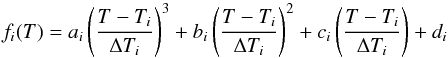 (C.1)where
ΔTi =
Ti + 1 −
Ti and, for
simplicity, we have dropped the index j spanning along the density grid. Cubic
polynomials are frequently used as they allow a set of data values to be smoothly fit with
specified derivatives at each endpoint. Although continuity of the first and second
derivatives across all polynomial segments are normally invoked when deriving the
coefficients of Eq. (C.1), we shall pursue
a different approach where
(C.1)where
ΔTi =
Ti + 1 −
Ti and, for
simplicity, we have dropped the index j spanning along the density grid. Cubic
polynomials are frequently used as they allow a set of data values to be smoothly fit with
specified derivatives at each endpoint. Although continuity of the first and second
derivatives across all polynomial segments are normally invoked when deriving the
coefficients of Eq. (C.1), we shall pursue
a different approach where 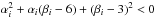 continuity is sacrificed in favor of monotonicity (Wolberg
& Alfy 2002). The resulting spline will be the smoothest curve that
passes through the control points while preserving monotonicity of the dataset but not
necessarily continuity of the second derivative. It can then be shown that the
coefficients are
continuity is sacrificed in favor of monotonicity (Wolberg
& Alfy 2002). The resulting spline will be the smoothest curve that
passes through the control points while preserving monotonicity of the dataset but not
necessarily continuity of the second derivative. It can then be shown that the
coefficients are  (C.2)where
 (C.3)The cubic is monotone if
there is no change in sign in the interval [
xi,xi
+ 1 ]. If this holds, then a necessary conditions is that
(C.3)The cubic is monotone if
there is no change in sign in the interval [
xi,xi
+ 1 ]. If this holds, then a necessary conditions is that
 (C.4)Defining
 and
and
 , and assuming that
mi ≠ 0, the sufficient
conditions for monotonicity can be summarized as follows:
, and assuming that
mi ≠ 0, the sufficient
conditions for monotonicity can be summarized as follows:
-
1.
Eq. (C.4) and αi + βi − 2 ≤ 0;
-
2.
Eq. (C.4) and αi + 2βi − 2 > 0 and one of the following conditions:
-
a)
2αi + βi − 3 ≤ 0;
-
b)
αi + 2βi − 3 ≤ 0;
-
c)
 .
.
-
a)
If monotonicity cannot be satisfied inside the interval or the spline does not have enough curvature, we simply revert to linear interpolation. A test for the latter condition is simply | d2fi(T) / dT2 | <ϵ | fi(T) | computed at the interval midpoint T = (Ti + Ti + 1) / 2 and ϵ = 10-16 is a small number.
All Tables
Summary of the chemistry reaction set. T is the temperature in Kelvin, TeV is the temperature in electron-volts, T5 = T/ 1 × 10⁵ and T2 = T/100.
Equations being solved when converting from pressure to internal energy (p → ρe) or vice versa (ρe → p).
All Figures
|
Fig. 1 Variation of mean molecular weight μ, internal energy density of the gas (ρe)gas and first adiabatic index Γ1 with temperature. The different colored curves represent four values of fixed density in g cm-3, viz., 10-4 (red), 10-8 (green), 10-12 (blue) and 10-16 (black). The values of (ρe)gas and Γ1 are obtained at equilibrium between ortho and para hydrogen. |
| In the text | |
|
Fig. 2 Different hydrogen fractions (XHI: atomic red, XH2: molecular green and XHII: ionized blue) obtained at equilibrium for different temperatures. We note that the total sum of fractions, i.e., XHI + 2XH2 + XHII is conserved. |
| In the text | |
|
Fig. 3 Top panel: variation with temperature of cooling function arising from different processes obtained using equilibrium values of hydrogen fractions (that vary with temperature as shown in Fig. 2) in units of erg cm3 s-1 for a total number density n0 = 105 cm-3. Bottom panel: different components of radiative cooling functions with same initial number density, n0 but for fixed values of concentration fractions (mentioned in the figure). In both panels, the sum of all the components is drawn with a black dashed line to obtain the value of Λ in erg cm3 s-1 following Eq. (32). |
| In the text | |
|
Fig. 4 Variation of density ρ (red), pressure P (green), and velocity vx (blue) along the x-axis (in code units) for a standard Sod Tube test (without explicit cooling) at time τ = 0.2. The values obtained using an ideal EoS are shown as solid lines while that obtained using a GammaLaw EoS are shown as dashed lines. |
| In the text | |
|
Fig. 5 Variation of density (left panels) and temperature (right panels) at the final stage of Sod shock tube test for cases which have included explicit cooling. The black line represent values obtained from ideal EoS, while those obtained using H/He EoS are shown in red. The top and bottom panels differ in the value of their initial temperature on either sides of the interface at x = 0.5. |
| In the text | |
|
Fig. 6 From top left to bottom right: solution at time t = 0.08 of density, pressure, internal energy density (ρe), temperature, X and Y components of velocity, Y component of magnetic field and adiabatic index respectively. In each panel, quantities obtained for ideal EoS are shown in (black) while the red line denotes values obtained using H/He EoS. |
| In the text | |
|
Fig. 7 Top panels: comparison of density ρ (in code units) for a hydrodynamic, spherical blast wave at time t = 0.15. Left panel: final shock structure with an ideal EoS. Top right panel: density obtained using the H/He EoS. Alongside each panel a zoomed in view of density around the contact discontinuity is shown. The ideal EoS shows presence of Rayleigh-Taylor instability while its completely absent in case of H/He EoS. Bottom panels from left to right: comparison of 1D cuts at the mid-plane of density ρ, pressure p, temperature (T/μ) and velocity (vx) for ideal EoS (black line) and H/He EoS (red line). |
| In the text | |
|
Fig. 8 Results from the test studying the propagation of supersonic pulsations in molecular medium. Top panel: comparison of density (in code units) for ideal EoS (black line) and H/He EoS (red line) on a log scale at time t = 192 yr. Bottom panels: comparison of zoomed up quantities for a particular knot marked within the rectangle in the top panel using the same color keys. These quantities from left to right are density ρ, pressure p, HI fraction XHI and temperature T/μ. A zoomed inset of the forward shock obtained from H/He EoS is shown as well with red dots to demonstrate the importance of resolving the shock (see text). |
| In the text | |
|
Fig. 9 Comparison of logarithmic values both of density, ρ (right half in blues) and temperature in Kelvin (left half in red) for a 2D axisymmetric jet without explicit cooling. The left panel shows the jet structure with an ideal EoS, while that obtained from a H/He EoS is shown in the right panel. |
| In the text | |
|
Fig. B.1 Comparisons between exact and tabulated approaches for the partially hydrogen gas
EoS. The black dashed line corresponds to computations obtained with the iterative
root-finder approach outlined in Sect. 3.2.1
while the red and green solid lines corresponds to the tabulated approach presented
in Sect. 3.2.2. Left: gas
internal energy (Eq. (B.1)) around
the transition region. Middle: fundamental gas derivative
|
| In the text | |
Current usage metrics show cumulative count of Article Views (full-text article views including HTML views, PDF and ePub downloads, according to the available data) and Abstracts Views on Vision4Press platform.
Data correspond to usage on the plateform after 2015. The current usage metrics is available 48-96 hours after online publication and is updated daily on week days.
Initial download of the metrics may take a while.