| Issue |
A&A
Volume 580, August 2015
|
|
|---|---|---|
| Article Number | A84 | |
| Number of page(s) | 8 | |
| Section | Planets and planetary systems | |
| DOI | https://doi.org/10.1051/0004-6361/201526218 | |
| Published online | 06 August 2015 | |
Using the chromatic Rossiter-McLaughlin effect to probe the broadband signature in the optical transmission spectrum of HD 189733b
1 Leiden Observatory, Leiden University, Postbus 9513, 2300 RA, Leiden, The Netherlands
e-mail: This email address is being protected from spambots. You need JavaScript enabled to view it.
2 Stellar Astrophysics Centre, Department of Physics and Astronomy, Aarhus University, Ny Munkegade 120, 8000 Aarhus C, Denmark
Received: 30 March 2015
Accepted: 23 June 2015
Abstract
Context. Transmission spectroscopy is a powerful technique for probing exoplanetary atmospheres. A successful ground-based observational method uses a differential technique that uses high-dispersion spectroscopy, but it only preserves narrow features in transmission spectra. Broadband features, such as the remarkable Rayleigh-scattering slope from possible hazes in the atmosphere of HD 189733b as observed by the Hubble Space Telescope, cannot be probed in this way.
Aims. Here we use the chromatic Rossiter-McLaughlin (RM) effect to measure the Rayleigh-scattering slope in the transmission spectrum of HD 189733b with the aim to show that it can be effectively used to measure broadband transmission features. The amplitude of the RM effects depends on the effective size of the planet, and in the case of an atmospheric contribution therefore depends on the observed wavelength.
Methods. We analysed archival HARPS data of three transits of HD 189733b, covering a wavelength range of 400 to 700 nm. The radial velocity (RV) time-series were determined for white light and for six wavelength bins each 50 nm wide, using the cross-correlation profiles as provided by the HARPS data reduction pipeline. The RM effect was first fitted to the white-light RV time series using the publicly available code AROME. The residuals to this best fit were subsequently subtracted from the RV time series of each wavelength bin, after which they were also fitted using the same code, leaving only the effective planet radius to vary.
Results. We measured the slope in the transmission spectrum of HD 189733b at a 2.5σ significance. Assuming it is due to Rayleigh scattering and not caused by stellar activity, it would correspond to an atmospheric temperature, as set by the scale height, of T = 2300 ± 900 K, well in line with previously obtained results.
Conclusions. Ground-based high-dispersion spectral observations can be used to probe broad-band features in the transmission spectra of extrasolar planets, such as the optical Rayleigh-scattering slope of HD 189733b, by using the chromatic Rossiter-McLaughlin effect. The precision achieved with HARPS per transit is about an order of magnitude lower than that with STIS on the Hubble Space Telescope. This method will be particularly interesting in conjunction with the new echelle spectrograph ESPRESSO, which currently is under construction for ESO’s Very Large Telescope, which will provide a gain in signal-to-noise ratio of about a factor 4 compared to HARPS. This will be of great value because of the limited and uncertain future of the Hubble Space Telescope and because the future James Webb Space Telescope will not cover this wavelength regime.
Key words: planets and satellites: atmospheres / techniques: radial velocities / methods: observational
© ESO, 2015
1. Introduction
Transmission spectroscopy has proven to be a powerful technique for probing the atmospheres of extrasolar planets (Charbonneau et al. 2002; Deming et al. 2013). Ground-based transmission spectroscopy is very challenging, even though telescopes with much larger collecting areas can be used than from space. Observations from the ground are hampered by the fact that a target is always seen through a varying amount of atmosphere. Moreover, atmospheric circumstances are never perfectly stable over a timescale of a few hours. In addition, instrument stability is crucial, since ground-based observations are subject to changes in the gravity vector and/or field rotation. One way to mitigate these issues is by using ground-based high-dispersion spectroscopy. For example, detections of sodium and potassium have been presented in the optical (Redfield et al. 2008; Snellen et al. 2008; Sing et al. 2011a; Wood et al. 2011; Jensen et al. 2011; Zhou & Bayliss 2012; Wyttenbach et al. 2015), and detections of carbon monoxide and water in the infrared (Brogi et al. 2012, 2014; Rodler et al. 2012; de Kok et al. 2013; Birkby et al. 2013; Lockwood et al. 2014).
Unfortunately, the high-dispersion spectroscopic technique is insensitive to broadband absorption features since only relatively narrow features can be probed because all large-scale structures in the spectra are removed during the data analysis to account for the telluric variability. Therefore, broadband features can only be probed from the ground using multi-object spectroscopy, which simultaneously observes the target and a number of reference stars to perform differential spectrophotometry to correct for atmospheric effects (Bean et al. 2010, 2011).
However, the most precise observations have been acquired from space. A particularly interesting broadband feature is the remarkable slope in the transmission spectrum of HD 189733b, as measured by Pont et al. (2008) and Sing et al. (2011b) using the Hubble Space Telescope (HST). Pont et al. (2013), who discussed the UV and optical spectrum based on a total of eight transits observed with STIS and ACS on the HST, found the radius of the planet to decrease by 1.5% between 345 nm and 775 nm. Lecavelier Des Etangs et al. (2008) and Pont et al. (2013) interpreted this slope as caused by Rayleigh scattering by hazes at a temperature of ~1300 K, possibly increasing to ~2000 K at the shortest wavelengths probing the lowest pressure region in the atmosphere. It would be extremely valuable if there were another way to probe this feature from the ground.
Snellen (2004) devised a method for probing the varying planet size as function of wavelength of a transiting exoplanet in a different way. The technique makes use of the Rossiter-McLaughlin (RM) effect. If the orbital plane of the planet is aligned with the spin of the star, the transiting exoplanet will first block light from the approaching part and then from the receding part of the stellar surface because the host star rotates. This effect results in a wobble in the radial velocity (RV) of the star, first seen by Rossiter (1924) for eclipsing binaries, and recently observed for transiting planets in many systems (e.g. Queloz et al. 2000). To first order, the overall amplitude of this effect, ARM, is proportional to  (1)where Vsini is the projected rotation velocity of the star, Rp is the planet radius, and Rstar is the stellar radius (Haswell 2010). As can be seen, this amplitude depends on the effective radius of the planet, and since this (in case of observable transmission features) is wavelength dependent, subsequently the amplitude of the RM effect is also wavelength dependent and can be measured (Snellen 2004). The advantage of this method over conventional transmission spectroscopy measurements is that instead of using the intensity of off-transit spectra as a reference for in-transit spectra, it depends on the changes in the profiles of the stellar spectral lines in the same on-transit spectra. For ground-based observation this makes the technique less likely to be influenced by Earth atmospheric effects, which turned out to be challenging for the conventional approach, because line shapes are less influenced by telluric absorption. Numerical simulations have been performed by Dreizler et al. (2009) to show the feasibility of this technique. Recently, Czesla et al. (2012) used a technique based on very similar principles to study the chromosphere of active planet host-stars.
While Snellen (2004) advocated this technique to probe narrow absorption features, such as those from sodium, we now realize that this method can be very powerful in probing wide broadband features, which are very challenging to probe from the ground. In this paper we test this technique on the exoplanet HD 189733b using archival HARPS data. In Sect. 2 the archival data and initial data analysis are described, and in Sect. 3 the models used to fit the RM effect are presented. In Sects. 4 and 5 we present the fit to the data and discuss the final results.
Planet orbital and stellar parameters used to calculate the Rossiter-McLaughlin (RM) effect with the AROME code (Boué et al. 2013).
2. HARPS data and radial velocity extraction
HD 189733b is a hot Jupiter with a mass of 1.15 MJupiter that orbits a K dwarf in 2.2 days. The system parameters used for our analysis are presented in Table 1. It is one of the two most frequently studied and observed exoplanets, together with HD 209458b. Its atmosphere has been observed both in trasmission and during secondary eclipses (e.g. Deming et al. 2006; Huitson et al. 2012; Wyttenbach et al. 2015).
We used HARPS archival data on HD 189733b, obtained under the programs 072.C-0488(E), 079.C-0828(A), and 079.C-0127(A). We chose not to use the data from 2006-07-29 because of the partial coverage of the transit (first half only) and because of the incomplete observation of the baseline. Instead, we used observations obtained during a total of three transits, which is the same dataset as was used by Wyttenbach et al. (2015), see their Table 1 for the observation logs. HARPS (Mayor et al. 2003) is a fibre-fed, cross-dispersed high-resolution (R ~ 115 000) echelle spectrograph at the ESO 3.6 m telescope, which through its stability is ideal for measuring RVs. It covers wavelengths from 378 nm to 691 nm over 72 orders. The data were taken during the night of September 7, 2006, consisting of 28 exposures of 600 s each, and on the nights of July 19, 2007 and August 28, 2007, consisting of 38 and 40 exposures of 300 s each, respectively. We retrieved the cross-correlation functions (CCFs) from the ESO archive. These CCFs are calculated by correlating the data with a binary mask, both computed for each order of the spectrograph and for the full wavelength range, which are standard products of the ESO archive. For comparison, we also used the values computed for the RV using the full wavelength range and the errors on these values. We note that the data reduction as used by the ESO archive used different masks for different nights, that is, a K5 mask for the first night and a G2 mask for the others. We used the data for the first night reduced with the G2 mask with the HARPS Data Reduction Software by Wyttenbach et al. (2015).
Wavelength passbands, the corresponding HARPS orders, and limb-darkening coefficients as used in our analysis.
2.1. RV extraction from the orders
To determine the RV as function of wavelength for each observed spectrum, we used the CCFs determined for each order of the HARPS spectrograph. We first combined the CCFs by averaging them, inside wavelength passbands of 50 nm chosen to be the same as used by Pont et al. (2008) and Sing et al. (2011b). These are shown in Table 2. In this way, we can keep the same limb-darkening coefficients as used in their studies and compare them directly. We note that the fourth and fifth passband overlap by half in wavelength because this is where the individual studies of Pont et al. (2008) and Sing et al. (2011b) overlap. The second column of Table 2 shows the range of HARPS orders in each passband. There is no exact match with the passbands used by Pont et al. (2008) and Sing et al. (2011b), but differences are negligible. The orders were assigned to the different passbands based only on their central wavelength. HARPS order 97 (central wavelength λ = 631.06 nm) was removed from our analysis because of strong telluric contamination from molecular oxygen absorption.
In this way, we obtained seven CCFs per spectrum for the seven different passbands. The RV extraction was performed as in the HARPS Data Reduction Software, that is, by fitting Gaussians to the CCFs. The centre of the Gaussian is the RV of that passband. This approach of averaging the CCFs in a passband before determining the RV is similar to the standard HARPS data reduction procedure, in which the CCFs from the different orders are first combined before they are fit with a Gaussian.
The photon-noise-limited uncertainty of a RV measurement is discussed by Hatzes & Cochran (1992), who showed that  (2)where σRV is the uncertainty in the RV, S is the flux, and R is the spectral resolution. The variable Δλ in practice is proportional to the number of spectral lines and their depths over the observed wavelength range. Since this is challenging to derive from first principles for the different passbands, we used the dispersion in the RV time-series to scale the errors afterwards.
3. Models for the Rossiter-McLaughlin effect
We used the publicly available code AROME (Boué et al. 2013) to analytically compute the RM RV anomaly as measured with the CCF method. This code, written in C, was given the orbital planetary and stellar parameters (the projected rotation velocity Vsin(i), the semi-major axis a, the radius of the star Rstar, expressed in solar radii units, the inclination angle i, the mutual inclination angle λ, and the planet orbital period P, all taken from Triaud et al. 2009, see Table 1), and the times of observation, which it subsequently used to calculate the CCFs and the expected RV measurements from a Gaussian fit to these. The fraction of flux blocked by a planet crossing the surface of its host star depends on the limb darkening of the star. For the calculation with AROME we chose the non-linear law of Claret (2000) to match those used in the analysis of Pont et al. (2008) and Sing et al. (2011b), that is,  (3)For the white-light RV time series we used the quadratic limb-darkening law coefficients as in Triaud et al. (2009), who studied the RM effect for this planet using the same data set. All the limb-darkening coefficients used in our analysis are given in Table 2. Since we are interested in the dependence of the RM effect on the planet effective size, for each passband we selected the limb-darkening law corresponding to those wavelengths and calculated the anomaly for 5000 values of the planet-star radius ratio (Rp/Rstar), between 0.105 and 0.205 with a step of 2 × 10⁻⁵. These boundaries were chosen arbitrarily with the purpose of including the measured planet-star radius ratio for this planet using the same HARPS data as Triaud et al. (2009) (0.1581 ± 0.0005). All other parameters were kept fixed. We note that for the analysis we are only interested in the relative change of the Rp/Rstar as function of wavelength, not in absolute values. Therefore it is not relevant to fit for parameters such as the projected rotation velocity Vsini, the mutual inclination angle λ, the macroturbulence z, and the scaled semi-major axis a/Rstar separately for each passband. These should be independent of wavelength and therefore can only result in a small vertical offset in the transmission spectrum, not in a change of slope.
4. Data analysis
The aim of our data analysis is to determine the change in the effective radius of the planet over the seven wavelength passbands. The first step in the analysis was to remove the RV variations due to the reflex motion of the host star around the planet-star barycenter. In addition, common mode errors that are expected to be similar over the whole wavelength range covered by HARPS were removed, since they will not influence the change in Rp/Rstar as function of wavelength. The final step is the retrieval of Rp/Rstar for the seven passbands.
4.1. Reflex motion of the star
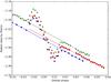 |
Fig. 1 White-light RV time series, plotted as blue dots for the first night, red squares for the second, and green triangles for the third night. The solid lines, with the same colours as used above, are the fitted reflex motion (K) and vsys for each night. These values are shown in Table 3. |
Assuming that the orbit of HD 189733b is circular, the RV motion of the host star vstar can be modelled as a sinusoid with semi-amplitude K and period P given in Table 1, plus a systemic RV vsys. The exact values of vsys differ from night to night because of the different stellar templates used to compute the CCFs (see Sect. 2). In addition, the RVs computed for the different passbands will also have small offsets because of the uncertainty in the reference RV for each order, see below. Stellar activity may also influence vsys by spots covering parts of the rotating stellar disk. In addition, star spots rotating in and out of view may also result in small differences in K between the nights (Albrecht et al. 2012). We performed a least-squares fit of the out-of-transit RV data to obtain K and vsys for each night. These values are shown in Table 3 and in Fig. 1.
Fitted values of the systemic velocity vsys and semi-amplitude of the reflex RV motion of the star, K for the three nights.
The reflex motion was subsequently removed from the white-light RV time series and from that of each passband. Small residual velocity offsets at a level of a few hundred meters per second were still present in the different passband RV time-series (since different parts of the templates were used). These offsets were also fitted and removed.
4.2. Removal of common mode errors from the data
Common mode errors that are identical across all passbands because of residual instrumental effects, star spots (to first order), stellar differential rotation, or other systematic effects (e.g. Triaud et al. 2009), can be removed from the data without harm. Therefore, we first performed a least-squares fit of the AROME models (Sect. 3) to the white-light RV time-series to determine the RM anomaly. This best fit was then removed from the white-light data to give the common mode errors on the time series, which were subsequently removed from the RV time series of each passband. To fit the white-light RV time series, a quadratic limb-darkening law was used with coefficients from Triaud et al. (2009), who analysed the same HARPS data as here. These coefficients are shown in Table 2.
To determine the best value of the radius ratio Rp/Rstar for the white-light RV time series, we computed the chi-squared χ2 for each model to the data, with the uncertainties rescaled such that the reduced χ2 of the best-fit model is equal to unity. The 1σ-confidence interval was then determined by selecting the values of the radius ratio at which Δχ2 = 1.
The best fit, shown in Fig. 2, yielded a planet/star radius ratio of Rp/Rstar = 0.1585 ± 0.0007, in agreement with the value found by Triaud et al. (2009) for this planet based on the same HARPS data (0.1581 ± 0.0005).
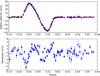 |
Fig. 2 Top panel: white-light RV time-series with the best fit to the Rossiter-McLaughlin anomaly. The fit yields a planet/star radius ratio of Rp/Rstar = 0.1585 ± 0.0007, in agreement with the measurement of Triaud et al. (2009). In the bottom panel the residuals to the fit are shown. These residuals contain information about possible star spots crossed by the planet during a transit and possible effects due to stellar differential rotation or macroturbulence. These residuals were subsequently removed from the RV time-series of the individual passbands. |
4.3. Fit of the Rossiter-McLaughlin curve
The resulting time series were fitted using the grid of models described in Sect. 3 by χ2 minimization. The uncertainties on the measurements were rescaled such that for the best fit  , and the associated 1σ errors were determined from the condition that Δχ2 = 1. We note that even if the limb-darkening coefficients chosen for each passband were wrong by a quarter of a passband width, this would only contribute to the uncertainty on the retrieved Rp/Rstar value on a level of less than 0.5σ.
Rp/Rstar values obtained for the different wavelength passbands.
5. Results
The least-squares fits to the RM effect in the individual passbands are shown in Fig. 3. The scatter of the residuals ranges from 2 m/s for the 470–520 nm passband to 9 m/s for the 650–700 passband. The Rp/Rstar obtained for the different wavelength passbands are given in Table 4 and are shown in Fig. 5. In Fig. 4 we show the data of the fifth passband with the best-fit model, and that for 5σ smaller and larger planet/star radius ratios to illustrate the sensitivity of our fitting method.
Star spots, unocculted by the planet, change the effective size of the star as function of wavelength. Therefore, they can have an equivalent effect on Rp/Rstar as a change in the effective size of the planet, which is what we wish to measure with transmission spectroscopy. Sing et al. (2011b) corrected for unocculted star spots by assuming a spot temperature of Tspot = 4250 ± 250 K, causing a stellar flux reduction of 1% at 600 nm. We performed that same analysis. However, because our uncertainties in Rp/Rstar are an order of magnitude larger, this spot correction contributes only at the 0.1σ level and was therefore ignored.
5.1. Rayleigh-scattering slope
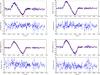 |
Fig. 3 Fit of the Rossiter-McLaughlin effect for all the individual wavelength bins (from top left to bottom right). In the top panels of each figure, the RVs are shown in blue, computed for each bin and in red the fit to them; in the bottom panels of each figure the residuals of the fit are shown. |
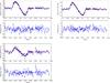 |
Fig. 3 continued. |
As in Sing et al. (2011b), Pont et al. (2008, 2013), we interpreted the optical transmission spectrum of HD 189733b as due to Rayleigh scattering. The Rayleigh scatter cross-section can be written as σ = σ0(λ/λ0)α, with α = −4, and therefore the slope of the planet radius as a function of wavelength is given by Lecavelier Des Etangs et al. (2008)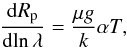 (4)where μ is the mean mass of the atmospheric particles, taken as 2.3 times the mass of the proton, k is the Boltzmann constant, and g the surface gravity. From the slope of the fit to the Rp/Rstar ratio as a function of the natural logarithm of the wavelength, an estimate of the atmospheric temperature (at pressures where the scattering takes place) can be derived.
We performed a least-squares fit for the data as shown in Fig. 5, weighting down the data points of passbands 520−570 nm and 550−600 nm by a factor 0.75 because they overlap by half. The best fit is shown in Fig. 5 and coresponds to a gradient of −0.0064 ± 0.0026 ln[Å]-1, which is significant at a 2.5σ level. Assuming Rstar = 0.766 R⊙ (Triaud et al. 2009), this gradient corresponds to an atmospheric temperature of T = 2300 ± 900 K (errors at 1σ confidence level).
We compared our results with those of Pont et al. (2013), who performed the combined analysis of the data in Sing et al. (2011b) and Pont et al. (2008). This is shown in Fig. 6. We note that we shifted the data from Pont et al. (2013) up by 0.0002 in Rp/Rstar to match our values. Our analysis is not meant to give precise absolute values of Rp/Rstar (which is influenced by the choices in stellar parameters such as projected rotational velocity and macro turbulence), only the relative change as function of wavelength. The uncertainties in our measurements are typically an order of magnitude larger than those of Pont et al. (2013).
Pont et al. (2013) inferred two different atmospheric temperatures for two separate wavelength regimes, below and above 550 nm. Above 550 nm they found a gradient that corresponds to a temperature of about 1300 K, while at shorter wavelengths the slope steepened corresponding to a temperature of about 2000 K. As can be seen in Fig. 6, the uncertainty in our data is too large to fit multiple slopes. The uncertainty in temperature found in our analysis agrees with both temperatures as found by Pont et al. (2013). The temperature in the upper atmosphere of HD 189733b has also been estimated usign the NaI doublet line cores. Huitson et al. (2012) used HST data and found a temperature of 2800 ± 400 K, while Wyttenbach et al. (2015) found a temperature of 2500 ± 400 K, using the same HARPS data set.
5.2. Other interpretations of the slope
In our analysis we assumed that the slope in the transmission spectrum of HD 189733 b is due to Rayleigh scattering, as was also assumed by Pont et al. (2008, 2013), Lecavelier Des Etangs et al. (2008), Sing et al. (2011b). However, in recent literature it has been advocated that star spots or plages might also result in the observed slope in the transmission spectrum. McCullough et al. (2014) reinterpreted the available measurements with a clear planetary atmosphere. They found that an unocculted spot fraction of 4% can mimic the increase in effective planet size towards shorter wavelengths. Occultation of stellar plages has also been claimed to be able to give rise to the slope in the spectrum of HD 189733b by Oshagh et al. (2014). We note that the chromatic RM effect as used in our analysis to determine the effective planet radius as function of wavelength is affected by star spots and/or plages in a similar fashion as classical transmission spectroscopy. Therefore, this analysis cannot contribute to this discussion at this stage.
However, it is worth noting that an increase in planetary radius towards UV wavelengths has been detected for a number of planets, for instance, GJ3470b (Nascimbeni et al. 2013; Biddle et al. 2014), WASP-6b (Nikolov et al. 2015), and WASP-31b (Sing et al. 2015). Interestingly, the host stars of all these planets and that of HD 189733b are active stars. This might indicate that unocculted star spots or plages may be the cause of this effect. Oshagh et al. (2014) also advocated this for the particular case of GJ3470b. A more detailed investigation is required to understand the relationship between stellar activity and slopes in transmission spectra of orbiting planets.
5.3. Future observations with ESPRESSO
We showed that with three transit observations of HD 189733b with HARPS, we obtained a relative precision of the planet radius as a function of wavelength, which is about an order of magnitude lower than that achieved for five transits with STIS at the HST (Pont et al. 2013). Since the chromatic RM technique is photon limited, a significant increase in precision can be expected from the forthcoming ESPRESSO spectrograph at ESO’s Very Large Telescope (Pepe et al. 2013).
We simulated future ESPRESSO observations by scaling the current accuracy achieved with HARPS by the increase in collecting area of the telescope and the increase in throughput of the ESPRESSO spectrograph, also taking into account the slight increase in spectral resolution to R = 120 000. The photon-noise contribution to the RV error is, according to Eq. (2), σRV ∝ S-0.5R-1.5, where S is the received flux from the star, and R the resolving power. Figure 7 shows the results of our simulation for five transits observed with ESPRESSO (blue squares) with their associated 1σ uncertainties. In red circles are shown the data points as presented by Pont et al. (2013) for also five transits observed with STIS. The expected uncertainties for ESPRESSO are about 1.5–2 times larger than for STIS. This is particularly important, taking into account the limited and uncertain future of the HST, and the fact that the future James Webb Space Telescope will not cover this wavelength regime.
We do note that the amplitude of the RM effect depends on the spin of the star and its angle with the planet’s orbit. Therefore, not all transiting planetary systems, for instance those orbiting slow rotators, are equally favourable for this technique.
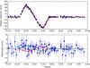 |
Fig. 4 Upper panel: RV time-series for the fifth passband (550–600 nm) and the corresponding best-fit model (blue dots and red line, respectively). Lower panel: residuals to the fit, together with the 5σ upper and lower limit of the Rp/Rstar ratio (solid red and green lines, respectively). |
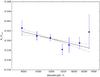 |
Fig. 5 Resulting planet-star radius ratio Rp/Rstar as function of wavelength, indicating the 1σ error bars. The solid line indicates the least-squares fit of a Rayleigh-scattering slope to the data, using Eq. (4). The dashed lines indicate the 1σ error margin on the slope. Note that the abscissae axis is in a logarithmic scale. The linear fit yields a gradient of −0.0064 ± 0.0026 ln[Å]-1, corresponding to a temperature of T = 2300 ± 900 K. |
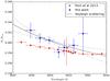 |
Fig. 6 Comparison of our Rp/Rstar measurements (blue squares) with those of Pont et al. (2013; red circles). The 1σ error bars are indicated. The solid and dashed lines are the same as in Fig. 5. |
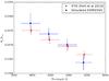 |
Fig. 7 Simulated Rp/Rstar for five transits observed with the future ESPRESSO spectrograph on the VLT (blue squares). Observations of five transits by the STIS spectrograph on HST as presented by Pont et al. (2013) are indicated by red circles. These are shifted slightly redward for clarity. All error bars indicate 1σ uncertainty intervals. These are larger by between 1.5 and 2 times for the ESPRESSO than for the STIS observations. |
6. Conclusion
We used the chromatic Rossiter-McLaughlin technique to probe the slope in optical transmission spectrum of HD 189733b using archival HARPS data. We showed that this technique can be used to measure this slope and found a change in radius ratio Rp/Rstar of −0.0064 ± 0.0026 ln[Å]-1 (2.5σ). Assuming this is due to Rayleigh scattering, it corresponds to an atmospheric temperature of T = 2300 ± 900 K.
The precision achieved with HARPS per transit is about an order of magnitude lower than that with STIS on the Hubble Space Telescope. This method will be particularly interesting in conjunction with the new echelle spectrograph ESPRESSO, which currently is under construction for ESO’s Very Large Telescope and will provide a gain in signal-to-noise ratio of about a factor 4 compared to HARPS. This will be of great value because of the limited and uncertain future of the Hubble Space Telescope and because the future James Webb Space Telescope will not cover this wavelength regime.
Acknowledgments
This work is part of the research programmes PEPSci and VICI 639.043.107, which are financed by the Netherlands Organisation for Scientific Research (NWO). Based on observations made with ESO telescopes at the La Silla Paranal Observatory under programme 072.C-0488(E), 079.C-0828(A), and 079.C-0127(A). We thank C. Lovis, A. Wyttenbach, D. Ehrenreich, and F. Pepe for useful discussion and insights.
References
- Albrecht, S., Winn, J. N., Johnson, J. A., et al. 2012, ApJ, 757, 18 [NASA ADS] [CrossRef] [Google Scholar]
- Bean, J. L., Miller-Ricci Kempton, E., & Homeier, D. 2010, Nature, 468, 669 [NASA ADS] [CrossRef] [PubMed] [Google Scholar]
- Bean, J. L., Désert, J.-M., Kabath, P., et al. 2011, ApJ, 743, 92 [NASA ADS] [CrossRef] [Google Scholar]
- Biddle, L. I., Pearson, K. A., Crossfield, I. J. M., et al. 2014, MNRAS, 443, 1810 [NASA ADS] [CrossRef] [Google Scholar]
- Birkby, J. L., de Kok, R. J., Brogi, M., et al. 2013, MNRAS, 436, L35 [NASA ADS] [CrossRef] [Google Scholar]
- Boué, G., Montalto, M., Boisse, I., Oshagh, M., & Santos, N. C. 2013, A&A, 550, A53 [NASA ADS] [CrossRef] [EDP Sciences] [Google Scholar]
- Brogi, M., Snellen, I. A. G., de Kok, R. J., et al. 2012, Nature, 486, 502 [NASA ADS] [CrossRef] [PubMed] [Google Scholar]
- Brogi, M., de Kok, R. J., Birkby, J. L., Schwarz, H., & Snellen, I. A. G. 2014, A&A, 565, A124 [NASA ADS] [CrossRef] [EDP Sciences] [Google Scholar]
- Charbonneau, D., Brown, T. M., Noyes, R. W., & Gilliland, R. L. 2002, ApJ, 568, 377 [NASA ADS] [CrossRef] [Google Scholar]
- Claret, A. 2000, A&A, 363, 1081 [NASA ADS] [Google Scholar]
- Czesla, S., Schröter, S., Wolter, U., et al. 2012, A&A, 539, A150 [NASA ADS] [CrossRef] [EDP Sciences] [Google Scholar]
- de Kok, R. J., Brogi, M., Snellen, I. A. G., et al. 2013, A&A, 554, A82 [NASA ADS] [CrossRef] [EDP Sciences] [Google Scholar]
- Deming, D., Harrington, J., Seager, S., & Richardson, L. J. 2006, ApJ, 644, 560 [NASA ADS] [CrossRef] [MathSciNet] [Google Scholar]
- Deming, D., Wilkins, A., McCullough, P., et al. 2013, ApJ, 774, 95 [NASA ADS] [CrossRef] [Google Scholar]
- Dreizler, S., Reiners, A., Homeier, D., & Noll, M. 2009, A&A, 499, 615 [NASA ADS] [CrossRef] [EDP Sciences] [Google Scholar]
- Haswell, C. A. 2010, Transiting Exoplanets [Google Scholar]
- Hatzes, A. P., & Cochran, W. D. 1992, in European Southern Observatory Conf. Workshop Proc. 40, ed. M.-H. Ulrich, 275 [Google Scholar]
- Huitson, C. M., Sing, D. K., Vidal-Madjar, A., et al. 2012, MNRAS, 422, 2477 [NASA ADS] [CrossRef] [Google Scholar]
- Jensen, A. G., Redfield, S., Endl, M., et al. 2011, ApJ, 743, 203 [NASA ADS] [CrossRef] [Google Scholar]
- Lecavelier Des Etangs, A., Pont, F., Vidal-Madjar, A., & Sing, D. 2008, A&A, 481, L83 [NASA ADS] [CrossRef] [Google Scholar]
- Lockwood, A. C., Johnson, J. A., Bender, C. F., et al. 2014, ApJ, 783, L29 [NASA ADS] [CrossRef] [Google Scholar]
- Mayor, M., Pepe, F., Queloz, D., et al. 2003, The Messenger, 114, 20 [NASA ADS] [Google Scholar]
- McCullough, P. R., Crouzet, N., Deming, D., & Madhusudhan, N. 2014, ApJ, 791, 55 [NASA ADS] [CrossRef] [Google Scholar]
- Nascimbeni, V., Piotto, G., Pagano, I., et al. 2013, A&A, 559, A32 [NASA ADS] [CrossRef] [EDP Sciences] [Google Scholar]
- Nikolov, N., Sing, D. K., Burrows, A. S., et al. 2015, MNRAS, 447, 463 [NASA ADS] [CrossRef] [Google Scholar]
- Oshagh, M., Santos, N. C., Ehrenreich, D., et al. 2014, A&A, 568, A99 [NASA ADS] [CrossRef] [EDP Sciences] [Google Scholar]
- Pepe, F., Cristiani, S., Rebolo, R., et al. 2013, The Messenger, 153, 6 [NASA ADS] [Google Scholar]
- Pont, F., Knutson, H., Gilliland, R. L., Moutou, C., & Charbonneau, D. 2008, MNRAS, 385, 109 [NASA ADS] [CrossRef] [Google Scholar]
- Pont, F., Sing, D. K., Gibson, N. P., et al. 2013, MNRAS, 432, 2917 [NASA ADS] [CrossRef] [Google Scholar]
- Queloz, D., Eggenberger, A., Mayor, M., et al. 2000, A&A, 359, L13 [NASA ADS] [Google Scholar]
- Redfield, S., Endl, M., Cochran, W. D., & Koesterke, L. 2008, ApJ, 673, L87 [NASA ADS] [CrossRef] [MathSciNet] [Google Scholar]
- Rodler, F., Lopez-Morales, M., & Ribas, I. 2012, ApJ, 753, L25 [NASA ADS] [CrossRef] [Google Scholar]
- Rossiter, R. A. 1924, ApJ, 60, 15 [NASA ADS] [CrossRef] [Google Scholar]
- Sing, D. K., Désert, J.-M., Fortney, J. J., et al. 2011a, A&A, 527, A73 [NASA ADS] [CrossRef] [EDP Sciences] [Google Scholar]
- Sing, D. K., Pont, F., Aigrain, S., et al. 2011b, MNRAS, 416, 1443 [NASA ADS] [CrossRef] [Google Scholar]
- Sing, D. K., Wakeford, H. R., Showman, A. P., et al. 2015, MNRAS, 446, 2428 [NASA ADS] [CrossRef] [Google Scholar]
- Snellen, I. A. G. 2004, MNRAS, 353, L1 [NASA ADS] [CrossRef] [Google Scholar]
- Snellen, I. A. G., Albrecht, S., de Mooij, E. J. W., & Le Poole, R. S. 2008, A&A, 487, 357 [NASA ADS] [CrossRef] [EDP Sciences] [Google Scholar]
- Triaud, A. H. M. J., Queloz, D., Bouchy, F., et al. 2009, A&A, 506, 377 [NASA ADS] [CrossRef] [EDP Sciences] [Google Scholar]
- Wood, P. L., Maxted, P. F. L., Smalley, B., & Iro, N. 2011, MNRAS, 412, 2376 [NASA ADS] [CrossRef] [Google Scholar]
- Wyttenbach, A., Ehrenreich, D., Lovis, C., Udry, S., & Pepe, F. 2015, A&A, 577, A62 [NASA ADS] [CrossRef] [EDP Sciences] [Google Scholar]
- Zhou, G., & Bayliss, D. D. R. 2012, MNRAS, 426, 2483 [NASA ADS] [CrossRef] [Google Scholar]
All Tables
Planet orbital and stellar parameters used to calculate the Rossiter-McLaughlin (RM) effect with the AROME code (Boué et al. 2013).
Wavelength passbands, the corresponding HARPS orders, and limb-darkening coefficients as used in our analysis.
Fitted values of the systemic velocity vsys and semi-amplitude of the reflex RV motion of the star, K for the three nights.
All Figures
|
Fig. 1 White-light RV time series, plotted as blue dots for the first night, red squares for the second, and green triangles for the third night. The solid lines, with the same colours as used above, are the fitted reflex motion (K) and vsys for each night. These values are shown in Table 3. |
| In the text | |
|
Fig. 2 Top panel: white-light RV time-series with the best fit to the Rossiter-McLaughlin anomaly. The fit yields a planet/star radius ratio of Rp/Rstar = 0.1585 ± 0.0007, in agreement with the measurement of Triaud et al. (2009). In the bottom panel the residuals to the fit are shown. These residuals contain information about possible star spots crossed by the planet during a transit and possible effects due to stellar differential rotation or macroturbulence. These residuals were subsequently removed from the RV time-series of the individual passbands. |
| In the text | |
|
Fig. 3 Fit of the Rossiter-McLaughlin effect for all the individual wavelength bins (from top left to bottom right). In the top panels of each figure, the RVs are shown in blue, computed for each bin and in red the fit to them; in the bottom panels of each figure the residuals of the fit are shown. |
| In the text | |
|
Fig. 3 continued. |
| In the text | |
|
Fig. 4 Upper panel: RV time-series for the fifth passband (550–600 nm) and the corresponding best-fit model (blue dots and red line, respectively). Lower panel: residuals to the fit, together with the 5σ upper and lower limit of the Rp/Rstar ratio (solid red and green lines, respectively). |
| In the text | |
|
Fig. 5 Resulting planet-star radius ratio Rp/Rstar as function of wavelength, indicating the 1σ error bars. The solid line indicates the least-squares fit of a Rayleigh-scattering slope to the data, using Eq. (4). The dashed lines indicate the 1σ error margin on the slope. Note that the abscissae axis is in a logarithmic scale. The linear fit yields a gradient of −0.0064 ± 0.0026 ln[Å]-1, corresponding to a temperature of T = 2300 ± 900 K. |
| In the text | |
|
Fig. 6 Comparison of our Rp/Rstar measurements (blue squares) with those of Pont et al. (2013; red circles). The 1σ error bars are indicated. The solid and dashed lines are the same as in Fig. 5. |
| In the text | |
|
Fig. 7 Simulated Rp/Rstar for five transits observed with the future ESPRESSO spectrograph on the VLT (blue squares). Observations of five transits by the STIS spectrograph on HST as presented by Pont et al. (2013) are indicated by red circles. These are shifted slightly redward for clarity. All error bars indicate 1σ uncertainty intervals. These are larger by between 1.5 and 2 times for the ESPRESSO than for the STIS observations. |
| In the text | |
Current usage metrics show cumulative count of Article Views (full-text article views including HTML views, PDF and ePub downloads, according to the available data) and Abstracts Views on Vision4Press platform.
Data correspond to usage on the plateform after 2015. The current usage metrics is available 48-96 hours after online publication and is updated daily on week days.
Initial download of the metrics may take a while.