| Issue |
A&A
Volume 580, August 2015
|
|
|---|---|---|
| Article Number | A125 | |
| Number of page(s) | 16 | |
| Section | Planets and planetary systems | |
| DOI | https://doi.org/10.1051/0004-6361/201525791 | |
| Published online | 17 August 2015 | |
MOA-2007-BLG-197: Exploring the brown dwarf desert⋆
1
Sorbonne Universités, UPMC Univ Paris 6 et CNRS, UMR 7095,
Institut d’Astrophysique de Paris, 98 bis bd Arago, 75014
Paris,
France
2
University of Canterbury, Dept. of Physics and Astronomy, Private Bag
4800, 8020
Christchurch, New
Zealand
3
Institute of Natural and Mathematical Sciences, Massey
University, Private Bag 102-904,
North Shore Mail Centre, Auckland, New Zealand
4
Department of Physics, University of Notre Dame,
Notre Dame, IN
46556,
USA
5
SUPA, School of Physics & Astronomy, North Haugh,
University of St Andrews, KY16
9SS, Scotland,
UK
6
Kavli Institute for Astronomy and Astrophysics, Peking
University, Yi He Yuan Road 5, Hai
Dian District, 100871
Beijing, PR
China
7
IRAP, CNRS – Université de Toulouse, 14 av. E. Belin, 31400
Toulouse,
France
8
CFHT Corporation, 65-1238 Mamalahoa Hwy,
Kamuela, Hawaii
96743,
USA
9
Department of Astronomy, Ohio State University,
140 W. 18th Ave., Columbus, OH
43210,
USA
10
School of Math and Physics, University of Tasmania,
Private Bag 37, GPO Hobart,
7001
Tasmania,
Australia
11
Niels Bohr Institutet, Københavns Universitet,
Juliane Maries Vej 30,
2100
København Ø,
Denmark
12
Space Telescope Science Institute, 3700 San Martin Drive, Baltimore, MD
21218,
USA
13
South African Astronomical Observatory,
PO Box 9, Observatory
7935, South
Africa
14
Department of Earth and Space Science, Graduate School of Science,
Osaka University, Toyonaka, Osaka
560-0043,
Japan
15
Qatar Environment and Energy Research Institute, Qatar
Foundation, PO Box
5825, Doha,
Qatar
16
Department of Physics, University of Rijeka,
Radmile Matej vcić 2,
51000
Rijeka,
Croatia
17
Technical University of Vienna, Department of
Computing, Wiedner Hauptstrasse
10, 1040
Wien,
Austria
18
Department of Physics, Chungbuk National University,
371-763
Cheongju,
Korea
19
Department of Physics and Astronomy, San Francisco State
University, 1600 Holloway
Avenue, San
Francisco, CA
94132,
USA
20 Korea Astronomy and Space Science Institute, 776
Daedukdae-ro, Daejeon, Korea
21
Las Cumbres Observatory Global Telescope Network,
6740 Cortona Drive, suite 102,
Goleta, CA
93117,
USA
22
Astronomisches Rechen-Institut, Zentrum für Astronomie
derUniversität Heidelberg (ZAH), Mönchhofstraße 12-14, 69120
Heidelberg,
Germany
23
Perth Observatory, Walnut Road, Bickley, 6076
Perth,
Australia
24
International Centre for Radio Astronomy Research, Curtin
University, Bentley,
WA
6102,
Australia
25
Solar-Terrestrial Environment Laboratory, Nagoya
University, 464-8601 Nagoya,
Japan
26
Okayama Astrophysical Observatory, National Astronomical
Observatory of Japan, 3037-5 Honjo,
Kamogata, Asakuchi, 719-0232
Okayama,
Japan
27
Nagano National College of Technology, 381-8550
Nagano,
Japan
28
Department of Physics, University of Auckland,
92019 Private Bag, 1010
Auckland, New
Zealand
29
Tokyo Metropolitan College of Aeronautics, 116-8523
Tokyo,
Japan
30
School of Chemical and Physical Sciences, Victoria
University, 6147
Wellington, New
Zealand
31
Institute of Information and Mathematical Sciences, Massey
University at Albany, Private Bag
102904, 0745 North Shore, Auckland, New Zealand
32
Mt. John University Observatory, PO Box 56, 8770
Lake Tekapo, New
Zealand
33
Department of Physics, University of Auckland,
Private Bag 92019, 1010
Auckland, New
Zealand
34
Department of Physics, Faculty of Science, Kyoto Sangyo
University, 603-8555
Kyoto,
Japan
Received: 2 February 2015
Accepted: 15 May 2015
Abstract
We present the analysis of MOA-2007-BLG-197Lb, the first brown dwarf companion to a Sun-like star detected through gravitational microlensing. The event was alerted and followed-up photometrically by a network of telescopes from the PLANET, MOA, and μFUN collaborations, and observed at high angular resolution using the NaCo instrument at the VLT. From the modelling of the microlensing light curve, we derived basic parameters such as, the binary lens separation in Einstein radius units (s ≃ 1.13), the mass ratio q = (4.732 ± 0.020) × 10-2 and the Einstein radius crossing time (tE ≃ 82 d). Because of this long time scale, we took annual parallax and orbital motion of the lens in the models into account, as well as finite source effects that were clearly detected during the source caustic exit. To recover the lens system’s physical parameters, we combined the resulting light curve best-fit parameters with (J,H,Ks) magnitudes obtained with VLT NaCo and calibrated using IRSF and 2MASS data. From this analysis, we derived a lens total mass of 0.86 ± 0.04 M⊙ and a lens distance of DL = 4.2 ± 0.3 kpc. We find that the companion of MOA-2007-BLG-197L is a brown dwarf of 41 ± 2 MJ observed at a projected separation of a⊥ = 4.3 ± 0.1 AU, and orbits a 0.82 ± 0.04 M⊙ G-K dwarf star. We then placed the companion of MOA-2007-BLG-197L in a mass-period diagram consisting of all brown dwarf companions detected so far through different techniques, including microlensing, transit, radial velocity, and direct imaging (most of these objects orbit solar-type stars). To study the statistical properties of this population, we performed a two-dimensional, non-parametric probability density distribution fit to the data, which draws a structured brown dwarf landscape. We confirm the existence of a region that is strongly depleted in objects at short periods and intermediate masses (P ≲ 30 d, M ~ 30−60 MJ), but also find an accumulation of objects around P ~ 500 d and M ~ 20 MJ, as well as another depletion region at long orbital periods (P ≳ 500 d) and high masses (M ≳ 50 MJ). While these data provide important clues on the different physical mechanisms of formation (or destruction) that shape the brown dwarf desert, more data are needed to establish their relative importance, in particular as a function of host star mass. Future microlensing surveys should soon provide more detections, in particular for red dwarf hosts, thus uniquely complementing the solar-type host sample.
Key words: planets and satellites: detection / gravitational lensing: micro / brown dwarfs
Figures 9–12 are available in electronic form at http://www.aanda.org
Corresponding author: A. Cassan, e-mail: This email address is being protected from spambots. You need JavaScript enabled to view it.
PLANET/RoboNET Collaboration.
MOA Collaboration.
μFUN Collaboration.
Deceased.
© ESO, 2015
1. Introduction
Gravitational microlensing is a powerful technique for detecting extrasolar planets (Mao & Paczynski 1991), and it holds great promise for detecting populations of brown dwarf companions to stars. Compared to other detection techniques, microlensing provides unique information on the population of exoplanets, because it allows the detection of very low-mass planets (down to the mass of the Earth) at long orbital distances from their host stars (typically 0.5 to 10 AU). It is also the only technique that allows discovery of exoplanets and brown dwarfs at distances from the Earth greater than a few kiloparsecs, up to the Galactic bulge, which would have been hard to detect with other methods.
Exoplanets are found to be frequent by all detection techniques (e.g., Cassan et al. 2012; Bonfils et al. 2013; Mayor et al. 2011; Sumi et al. 2011; Gould et al. 2010b), and recent statistical microlensing studies even imply that there are, on average, one or more bound planets per Milky Way star (Cassan et al. 2012). Conversely, brown dwarfs appear to be intrinsically rare, to the point that shortly after the first exoplanet detections, it led to the idea of a “brown dwarf desert” (Marcy & Butler 2000) bridging the two well-defined regions of binary stars and planetary systems. While in the past, brown dwarfs were defined as objects of mass within the deuterium- and hydrogen-burning limits (13−74 MJ, Burrows et al. 2001), it appears today that different formation scenarios can build objects with similar masses but with different natures (super-massive planets, or low-mass brown dwarfs). An object formed via core accretion and reaching 13 MJ would, for example, be able to start deuterium burning, as would an object of same mass formed by gravitational collapse of a cloud or in a protoplanetary disk (Mollière & Mordasini 2012).
Despite their low occurrence, a number of brown dwarf companions to stars have been discovered by different methods: radial velocity and transit (e.g., Moutou et al. 2013; Díaz et al. 2013; Sahlmann et al. 2011; Johnson et al. 2011; Deleuil et al. 2008), direct imaging (e.g., Lafrenière et al. 2007) and microlensing. With regards to microlensing, there are still a few brown dwarf detections, but this is mainly because until now observing priority has been given to exoplanets. Nevertheless, these detections are of particular interest because they provide a unique view of brown dwarfs around low-mass stars (mainly M dwarfs), which complements the currently available sample mostly composed of solar-type stars.
Microlensing detections so far include isolated brown dwarfs, brown dwarfs hosting planets, and brown dwarf companions to stars. The first isolated brown dwarf detected through gravitational microlensing (a 59 ± 4 MJ brown dwarf located at 525 ± 40 pc in the thick disk of the Milky Way) was reported by Gould et al. (2009) in microlensing event OGLE-2007-BLG-224. Two brown dwarfs with planetary-mass companions were discovered in events OGLE-2009-BLG-151/MOA-2009-BLG-232 and OGLE-2011-BLG-0420 by Choi et al. (2013). In both cases, the planets were super Jupiters (7.9 ± 0.3 MJ and 9.9 ± 0.5 MJ, respectively) with the hosts being low-mass brown dwarfs (19 ± 1 MJ and 26 ± 1 MJ, respectively), with very tight orbits (below 0.4 AU). Similarly, Han et al. (2013) report a 23 ± 2 MJ field brown dwarf hosting a 1.9 ± 0.2 MJ planet in a tight system after the analysis of the event OGLE-2012-BLG-0358.
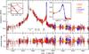 |
Fig. 1 Upper panel: the light curve of MOA-2007-BLG-197 and the best-fit model (solid line) with a zoom on the caustic exit on the right-hand side. On the left-hand side, the structure of the resonant caustic is drawn in red, as well as the trajectory of the source, in black (axes are in Einstein radius units). The source is too small to be distinguished. The four intervals E1−4 indicate time intervals where possible source caustic crossing (caustic entry) have been investigated. Lower panel: the residuals of the best-fit model. |
The first published microlensing detection of a brown dwarf companion to a star is OGLE-2008-BLG-510/MOA-2008-BLG-369, which was first reported by Bozza et al. (2012) as an ambiguous case between a binary-lens and a binary-source event. The data were reanalysed by Shin et al. (2012a), who concluded that the binary-lens model involving a massive brown dwarf orbiting an M dwarf was preferred. Shin et al. (2012b) conducted a database search for brown dwarf companions by focusing on microlensing events that exhibit low mass ratios. Among seven good candidates with well-determined masses (combination of Einstein radius and parallax measurements), they found two events that involve brown dwarfs: OGLE-2011-BLG-0172/MOA-2011-BLG-104 with mass 21 ± 10 MJ around an M dwarf, and MOA-2011-BLG-149, a 20 ± 2 MJ brown dwarf also orbiting an M dwarf. Similarly, Bachelet et al. (2012) reported the detection of another ~52 MJ brown dwarf orbiting an M dwarf in MOA-2009-BLG-411, although the lens mass could not be determined exactly, and was estimated through statistical realisations of Galactic models. In microlensing event MOA-2010-BLG-073, Street et al. (2013) find that the lens was composed of a 11.0 ± 2.0 MJ companion (hence near the planet/brown boundary) orbiting an M dwarf of 0.16 ± 0.03 M⊙. Jung et al. (2015) report the detection of a star at the limit of the brown dwarf regime hosting a companion at the planet/brown dwarf boundary (13 ± 2 MJ). More recently, Park et al. (2015) have reported the discovery of a binary system composed of a 33.5 ± 4.2 MJ brown dwarf orbiting a late-type M dwarf in microlensing event OGLE-2013-BLG-0578.
Here we report the first microlensing discovery of a brown dwarf orbiting a Sun-like star. This new brown dwarf has a mass of 42 MJ and it was observed at a projected separation of 4.3 AU from its G-K dwarf host star.
In Sect. 2, we present photometric data collected on MOA-2007-BLG-197L by several round-the-world telescopes, as well as high resolution adaptative optics images taken with NaCo at VLT. In Sect. 3, we present the full analysis of the light curve and in Sect. 4 we derive the physical parameters of the lens by combining all independent informations. In Sect. 5, we adopt a statistical point of view to analyse the current population of brown dwarfs detected with different methods using non-parametric probability density estimation tools. In Sect. 6 we summarise our results, and underline the importance of future microlensing observations to characterise the populations of objects in the mass region between planets and stars.
2. Observational data
2.1. Alert and follow-up
MOA-2007-BLG-197 (l = 359.711, b = −5.509, or RA (J2000) = 18:07:04.729, Dec (J2000) = −31:56:46.77) is a microlensing event that was alerted by the MOA collaboration (1.8 m telescope located in Mount John, New Zealand) in 2007 May 28 (or THJD ≃ 42491 on the photometric light curve shown Fig. 1). Soon after, between 1−5 June (THJD ≃ 4251−4255), a very cloudy weather in New Zealand seriously affected the quality and reliability of the photometry, resulting in gaps in the time series. A magnification peak in the MOA light curve was passed around June 6 (THJD ≃ 4258). On June 8 (THJD ≃ 4259.7), the PLANET collaboration added the event to its target list as a regular mid-magnification object. Follow-up observations include data from the PLANET network using the Danish telescope 1.54 m at La Silla (Chile), Canopus 1m in Hobart (Tasmania), SAAO 1 m in Sutherland (South Africa) and Perth 0.6 m telescope (Australia), while the μFUN collaboration collected data from CTIO 1.3 m in Mount Cerro Tololo (Chile).
On June 19 (THJD ≃ 4272), PLANET observers noticed that a few MOA data points were slightly above the standard single-lens theoretical curve. As this usually happens quite often in microlensing data, no alert was released. Indeed SAAO soon revealed that the alleged deviation was a false alert, but follow-up observations were continued. On July 5 (THJD ≃ 4287), even though the full moon affected the quality of the observations, a public alert was issued after Danish 1.54 m data were found to be above the single lens curve by more than 0.2 mag for more than five consecutive days. Intensive follow-up observations from SAAO confirmed the rise in brightness, announcing a caustic crossing. While Perth was overclouded, Canopus then took over, and was the only telescope to densely cover the caustic exit, which took place during the night of July 4 in Australia (THJD ≃ 4287.0−4287.4, see inset of Fig. 1).
Telescopes and photometric data sets.
2.2. Photometric light curve
The photometric data was reduced several times using different software to check their consistency. The final lightcurve data from all telescopes were extracted with the PLANET pipeline PySIS (Albrow et al. 2009), which is a DIA-based algorithm (Difference Image Analysis, Alard 2000; Alard & Lupton 1998). For images taken in particularly bad weather conditions, we examined by eye each image in order to check whether the subtraction was correct or not. In the latter case we had to exclude them, but on the basis of image quality only. In the post-processing of the reduced data, we applied a cut in seeing and sky background, although in a very conservative way so that possible low-amplitude signals were not rejected. Not surprisingly, most of the data taken by MOA during the very bad weather period mentioned before (THJD ≃ 4251−4255) had to be discarded. Unfortunately, a critical light curve feature is thereby not covered (which has important consequences, see Sect. 3), however there was no other choice but to remove these data, as they might otherwise have affected the reliability of our models.
The final light curve data amounts to a total of 802 data points. They are summerised in Table 1. As seen in the table, all telescopes use a similar I-band filter, apart from the MOA 1.8 m telescope which is equipped with a broad R/I filter (referred to as RM). Additionally, a few V-band images were taken by PLANET and μFUN to produce colour-magnitude diagrams (see Sect. 4.1).
The last concern about the photometry was the estimation of the error bars of the data. Galactic bulge fields are highly crowded with stars, and during a microlensing event, the flux variation can easily span two order of magnitudes for high-magnification events. These pose severe challenges to manage a good estimation of the error bars. As a matter of fact, in microlensing experiments it is long known that data reduction software usually underestimates error bars. Furthermore, error bars can vary significantly from one data set to another, with the risk that one data set dominates over the others at the modelling stage. A relatively robust method to prevent these drawbacks is to rescale the error bars, based on the best model fitting the data. For each data set, the (classical) χ2 is set up to the number of degrees of freedom by adjusting a rescaling factor f in the formula  , where σ′ and σ are respectively the rescaled and initial error bars on the magnitudes, and σ0 = 4 × 10⁻⁴ a constant accounting for the data most highly magnified. The f factors are given in Table 1 for each data set.
2.3. VLT NaCo high resolution images
On the night 20/21 of August 2007 (THJD ≃ 4333.0) we obtained first epoch observations2 of high resolution adaptive optics (AO) images in the near-infrared bands J, H and Ks using the NaCo instrument, mounted on 8.2 m ESO VLT Yepun telescope (Fig. 2). The source star was then still magnified by a factor of about A ≃ 1.30. A year later, on the night 2008 August 3/4 (THJD ≃ 4682.1), we carried out second epoch observations3 while the event was back to baseline magnitude. In principle, when two epochs are obtained at different magnifications, it should be possible to directly disentangle the lens flux from the source flux. In our case, however, the combination of a relatively high blending factor and low magnification did not support this direct measurement. Therefore, in the global analysis we used only the first epoch images. We reduced and calibrated the NaCo images following the general method outlined in Kubas et al. (2012) and briefly described below.
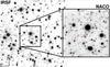 |
Fig. 2 Left: sub-region (94″ × 77″) of an original 3′ × 3′Ks-band IRSF image used to calibrate the NaCo magnitudes. Right: corresponding Ks-band NaCo image (27″ × 25″) used to cross-identify the stars. |
The night was clear and stable according to the observatory night logs, and the target was observed at low airmass and in good seeing conditions (<0.8″). The data were taken in auto-jitter mode within a 10″ jitter box including the target in order to be able to correct for bad pixels and sky background. The AO correction was done using a K = 11.17 ± 0.02 mag star (2MASS 18070464-3156423) at an angular separation of about 5″ from the microlensing target. The data were dark subtracted, flat-fielded and co-added with the tools underlying the NaCo pipeline software (Devillard 1999).
To derive the photometry from the reduced data, the first step was to compute the zeropoints for the conversion of instrumental magnitudes to calibrated magnitudes. A first possibility was to use catalogued stars within the target frame field-of-view (FOV), in our case 28″ × 28″. While several cross-matches between the NaCo frames and the 2MASS catalogue were identified, only 2MASS 18070520-3156409 (J = 14.24 ± 0.05, H = 13.69 ± 0.05, K = 13.48 ± 0.05) turned out as suitable (other potential calibrators in the NaCo images were either saturated or in the nonlinear regime of the detector). We finally checked that this star was not variable, by comparing a series of H-band images taken with Andicam at CTIO, which is well calibrated to 2MASS thanks to its 2.4′ × 2.4′ FOV. A second option for calibration was to use the zeropoints derived from the photometric standards taken with NaCo directly before the observations on the night 20/21 of August and at similar airmass. For calibration we used J,H,K magnitudes4 of star 9160-S870-T in the listed standards of Persson et al. (1998), which had the following advantages: this star was brighter than the previous 2MASS reference, and the smaller pixel scale made it less sensitive to blending contamination in our crowded field. For consistency, however, we measured the magnitude of 2MASS 18070520-3156409 in the NaCo frame, and found an agreement to better than 3%.
The second step was to extract accurate photometry from AO images in the infrared. This was not a straightforward task, since the shape of the point-spread function (PSF) often is not well fitted by analytical profiles, and also depends on the position of the target with respect to the star used for AO correction. Following Kubas et al. (2012), we constructed a PSF reference directly from stars in the NaCo frame, using the StarFinder package (Diolaiti et al. 2000). This software was especially designed for AO images of crowded stellar fields. We found J = 17.68 ± 0.06, H = 17.05 ± 0.05 and Ks = 16.87 ± 0.05. The quoted error bars are dominated by the uncertainties in determining the true PSF shape and the scatter of the sky and unresolved background sources. The measurements obtained with StarFinder are summarised in Table 2.
Derived NaCo magnitudes of the microlensing event target in the (J,H,Ks) filters for the two epochs 2007 August 20/21 (epoch 1) and 2008 August 3/4 (epoch 2).
The final step consisted in correcting the target for interstellar extinction, by fitting the position of the red clump giants (RCG) in the three colour-magnitude diagrams (CMD) involving the measured J,H,Ks reddened magnitudes. Because the nominal range in magnitudes from NaCo is above the 2MASS faint limit, we performed InfraRed Survey Facility (IRSF) observations at SAAO to extend the available 2MASS star list into the regime of stars measured within the NaCo frame. We used Kato et al. (2007) to obtain the calibration of IRSF images with respect to the 2MASS reference-star catalogue, noting that Janczak et al. (2010) found that no additional colour term is needed between NaCo and IRSF filters (the full process to build the calibration ladder is detailed in Kubas et al. 2012). Data to construct the NaCo+IRSF CMD are extracted from 2304 stars identified within a 3′ circle around the target in IRSF images, and 135 stars identified in the NaCo images (Fig. 2). The resulting de-reddened and calibrated CMD is plotted in Fig. 3, with a fit of the Red Clump Giant (RCG) position using a 10 Gyr, Z = 0.019 isochrone from Bressan et al. (2012), and assuming a RCG distance modulus of μ = 14.6 mag. This distance modulus is longer than the value used in Kubas et al. (2012) since the event is located in the Galactic bar (see Sect. 4.1 for a detailed discussion). From this analysis, we derived the following extinctions: AJ = 0.51 ± 0.05 mag, AH = 0.33 ± 0.05 mag and AKs = 0.22 ± 0.05 mag. These data are used in Sect. 4.2 to constrain the lens and mass distance.
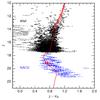 |
Fig. 3 (J,J − Ks) colour–magnitude diagram in the 2MASS system combining NaCo and IRSF data (respectively, in blue and black). The red dot is the magnitude/colour of the source derived from the source characterisation (Sect. 4.1). The values are not corrected for interstellar extinction. The red clump (RCG) is fitted by the red over-plotted 10 Gyr, solar-metallicity isochrone from Bressan et al. (2012). |
3. Light curve modelling
3.1. Binary lens parameters
We start by modelling the light curve of MOA-2007-BLG-197 with a static binary-lens model, in order to identify broad classes of possible solutions. In this model, the lens is characterised by its binary mass ratio q, and s, the projected separation of the binary lens in angular Einstein radius units θE. Here, 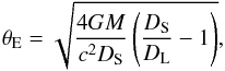 (1)where G is the gravitational constant, c the speed of light, DL and DS are respectively the observer-lens and observer-source distances and M the total mass of the lens. Four additional parameters describe the source mean rectilinear motion: the minimum impact distance u0 between the source and the origin (here, the centre of mass of the system, with the more massive body on the right-hand side), t0, the date at which the source reaches u0, tE, the time it takes for the source to travel one Einstein angular radius, and α, the angle between the source trajectory and the lens symmetry axis.
When the source approaches a caustic, finite-source effects cannot be neglected and substantial deviations from a point-source model are expected. Finite-source effects are included in the modelling through  (2)where θS is the angular radius of the source, and ρ the same quantity but in Einstein radius units. Here and in the following, a point-source model is used when the source is far enough from the caustics (t ≤ 4240.0 and t ≥ 4300.0); closer to the caustics, a hexadecapole approximation to the finite-source magnification (Gould 2008) is used (t ∈ [ 4240.0,4247.9 ] ∪ [ 4260.0,4286.0 ] ∪ [ 4287.5,4300.0 ]), until it breaks down, approximately when the source is closer than ~3ρ from the caustics. In this case, a full integration along the source images contours (Dominik 2007; Bozza 2010; Gould & Gaucherel 1997) or ray-shooting of the images are required (Dong et al. 2006, 2009; Bennett 2010) to compute the magnification. Since finite-source effects dramatically increase the computational cost, these time intervals are reduced as much as possible (here, t ∈ [ 4247.9,4260.0 ] ∪ [ 4286.0,4287.5 ]).
Microlensing light curves are usually sensitive to stellar limb darkening (e.g., Albrow et al. 1999b; Cassan et al. 2006). We thus model the source as a linear limb-darkened disk (An et al. 2002; Zub et al. 2011) described by the intensity-normalised profile ![Mathematical equation: \begin{equation} I(r) = \frac{1}{\pi}\left[ 1- \Gamma \left( 1-\frac{3}{2} \sqrt{1-r^2} \right) \right], \end{equation}](/articles/aa/full_html/2015/08/aa25791-15/aa25791-15-eq130.png) (3)where 0 ≤ r ≤ 1 is the fractional radius, and Γ the linear limb-darkening (LLD) coefficient. While in special cases limb-darkening laws beyond the linear law may slightly improve the model (e.g., Cassan et al. 2004; Kubas et al. 2005), in the case of MOA-2007-BLG-197L (relatively sparse data coverage of the caustic crossings) it is an excellent approximation. As seen in the right inset of Fig. 1, only Canopus data are sensitive to limb darkening, although the light curve sampling is not dense enough to provide strong constraints on the LLD coefficient. We therefore use Claret & Bloemen (2011) for the source surface gravity and effective temperature found in Sect. 4.1 (log g ~ 4.47, Teff ~ 5350 K) to estimate MOA-2007-BLG-197L LLD coefficients, and found ~0.4 for the I filter and ~0.5 for the R filter. We checked that refining the Canopus-I LLD coefficient with a fit to the data leads to ΓI = 0.48. We then adopted ΓI = 0.48 for all I-band data and ΓRM = 0.5 (MOA ΓRM filter is a broad R/I filter).
(3)where 0 ≤ r ≤ 1 is the fractional radius, and Γ the linear limb-darkening (LLD) coefficient. While in special cases limb-darkening laws beyond the linear law may slightly improve the model (e.g., Cassan et al. 2004; Kubas et al. 2005), in the case of MOA-2007-BLG-197L (relatively sparse data coverage of the caustic crossings) it is an excellent approximation. As seen in the right inset of Fig. 1, only Canopus data are sensitive to limb darkening, although the light curve sampling is not dense enough to provide strong constraints on the LLD coefficient. We therefore use Claret & Bloemen (2011) for the source surface gravity and effective temperature found in Sect. 4.1 (log g ~ 4.47, Teff ~ 5350 K) to estimate MOA-2007-BLG-197L LLD coefficients, and found ~0.4 for the I filter and ~0.5 for the R filter. We checked that refining the Canopus-I LLD coefficient with a fit to the data leads to ΓI = 0.48. We then adopted ΓI = 0.48 for all I-band data and ΓRM = 0.5 (MOA ΓRM filter is a broad R/I filter).
Finally, two additional parameters,  (source flux) and
  (blended flux), are included per individual observatory or filter, so that for a given individual data set i the total flux of the microlensing target reads
  (4)where A(t) is the time-dependent source flux magnification factor. The blending flux FB accounts for all luminous contributions other than the source, in particular, it includes the flux from the lens. For the best model presented in Table 3, the blending flux ratios FB/FS are respectively 17.79 (MOA), 38.14 (SAAO), 12.85 (CTIO), 3.97 (Canopus), 66.97 (Perth), 12.10 (Danish). The high value for Perth is easily explained by the fact that the aperture of the telescope is small and the seeing was relatively high, which results in a higher blend fraction.
Best-fit solutions for the different models of MOA-2007-BLG-197.
3.2. Caustic-crossing parametrisation
The shape of the MOA-2007-BLG-197 light curve (Fig. 1) clearly indicates that the source crosses (i.e., exits) a fold caustic at THJD ≃ 4287.2, mainly thanks to Canopus data densely covering this part of the light curve. On the other hand, the date of the caustic entry is ambiguous. In fact, for such a small angular source size as suggested by the caustic exit, the caustic entry could easily fit in one of the several gaps in the data coverage, in particular those marked as E1−4 in Fig. 1.
One of the modelling challenges for this event was to find all possible local minima involving all possible caustic entry dates. The problem with the set of parameters (u0,α,tE,t0) described in the previous section is that it is not well suited to explore efficiently the parameter space. In fact, only very special combinations of these parameters produce caustic crossings at the right locations on the light curve. Albrow et al. (1999a) proposed for the first time to introduce specific parameters to model a caustic crossing. Cassan (2008) developed further this approach, and generalised it to a pair of caustic crossings (entry and exit) by introducing a specific parametrisation of the caustic curves. This method is particularly efficient for an event like MOA-2007-BLG-197.
In this formalism, two alternative parameters tin and tout are used to fit for the dates of the source entry (in) and exit (out), while two other parameters sin and sout (which are curvilinear distances along the caustic curve) are used to fit for the source centre ingress and egress points on the caustic. It has been demonstrated that this parametrisation is more efficient in locating all possible fitting source-lens trajectories (Kains et al. 2009, 2012), because they all produce caustic-crossing features at the observed dates. Cassan et al. (2010) later derived Bayesian priors on parameters (tin,tout,sin,sout) to explore even more efficiently the parameter space. The best-fit values derived from the minimisation process are finally converted back to the classical parameters.
We explored5 all static binary-lens models using this parametrisation for all possible source caustic crossing dates within the E1 to E4 intervals displayed in Fig. 1, and for a regular (log s,log q) grid of 30 × 30 spanning log (0.4) ≤ log s ≤ log (4) and −4 ≤ log q ≤ 0. The minimisation was performed using a classical Markov Chain Monte Carlo (MCMC) algorithm. The best model involves a caustic entry in the time interval E1, the longest of the four gaps explored. The best-fit values of the model parameters and the corresponding χ2 are listed in column ESBL (Extended-Source, Binary-Lens) of Table 3, and posterior probability densities (correlation plots) are presented in Fig. 9.
3.3. Annual parallax
Given the long timescale found previously for the static binary lens model (tE ~ 80 days), this event is a priori likely to exhibit annual parallax effects. The relative lens-source (annual) parallax is expressed as  (5)so that the Einstein angular radius Eq. (1) also reads
  (6)where κ ≃ 8.144 mas /M⊙. The Einstein parallax vector πE has an amplitude
  (7)and a direction along the lens-source proper motion. As fitting parameters, it is convenient to decompose πE into a northwards component πE,N and an eastwards component πE,E (An et al. 2002), with advantages discussed in Gould (2004).
The best-fit model including parallax only (besides the parameters described in Sect. 3.1) is presented in column ESBL+P of Table 3, and correlation plots are shown in Fig. 10. It can be noticed that the binary mass ratio q and separation s change little by including parallax compared to ESBL, resulting in a very similar resonant caustic structure. As expected, including parallax in the model improves the χ2, by around 100. Nevertheless, we found that several solutions with very different values of parallax (between 0.8 to 1.5) give almost identical χ2 differing by only one or two units. The differences between these models come from differences in the caustic entry date tin, i.e. precisely where no data are available to constrain the model. Hence, although parallax improves the fit, it is unlikely that a workable measurement can be obtained (we discuss this further later).
3.4. Orbital motion
Orbital motion of the lens is also a priori likely to produce noticeable effects, because the event is fairly long and the caustic resonant. The orbital rotation of the two lens components affects the caustic in two ways: it changes the projected binary separation s and the orientation of the caustic in the plane of the sky. To first order, one can write s(t) ≃ s + ṡ (t − tr) and  , where tr is an arbitrary reference date chosen close or equal to t0. These two effects are included in the model through parameters γ∥ = ṡ/s and
  , with
  .
.
The best-fit model including lens orbital motion with ESBL is presented in column ESBL+LOM of Table 3 (correlation plots are shown in Fig. 11). According to this model, the changes in the caustic geometry are very slow, which should result in a poor signature on the light curve. Therefore, while this model also provides a better fit than ESBL alone (Δχ2 = 93), it is unlikely to give a good constraint on the lens orbital motion. Furthermore, the Δχ2 between this model and ESBL+P (parallax alone) is only lower than 10 although two more parameters have been included in the model. We conclude that the key time intervals for disentangling orbital motion from parallax are not covered densely enough by the data.
3.5. Annual parallax and orbital motion
As (annual) parallax and orbital motion individually lead to a similar improvement of the ESBL χ2, we now include both effects in the model to check whether a better χ2 can be found. Parallax and orbital motion are known to be very correlated (Batista et al. 2011; Skowron et al. 2011).
We investigate the two cases u0> 0 and u0< 0 (columns ESBL+P+LOM of Table 3) to check for possible ecliptic degeneracy (Skowron et al. 2011), and find that u0> 0 is preferred by Δχ2 = 11.9. The ESBL best-fit parameters, again, are relatively stable. The correlation plots of the best model are shown in Fig. 12. As expected, the overall fit is not significantly better than ESBL+P (Δχ2 = 12.2) or ESBL+LOM alone (Δχ2 = 20.5). This is consistent with a strong degeneracy between these parameters, that cannot be reliably broken in the case of MOA-2007-BLG-197.
3.6. Summary and conclusions from the modelling
A model with (annual) parallax improves the goodness-of-fit by Δχ2 ~ 100 compared to a static binary lens, but several models with very different values of πE give comparable values of χ2. Moreover, models with parallax or orbital motion alone lead to comparable χ2. This is not surprising for two reasons. Firstly, the caustic entry is not well covered by the data and it appears that a high value of parallax tends to change substantially the time of the caustic entry inside E1. Secondly, parallax effects are partly degenerate with lens orbital motion, and the available data sets are not sufficient to disentangle these two effects.
We therefore adopt the ESBL parameters (s,q,u0,α,tE,t0) found for model ESBL+P+LOM and u0> 0. Following the arguments summarised in the previous paragraph, other parameters such as parallax or orbital motion parameters cannot be used to constrain the lens mass and distance.
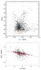 |
Fig. 4 Upper panel: (I,V − I) Danish instrumental CMD of the field around MOA-2007-BLG-197, not corrected for interstellar extinction. The red point marks the position of the RCG. The magnitude of the microlensing target is in blue (i.e. magnified source, lens and blended light). The orange point corresponds to the source alone. Lower panel: empirical linear relation between instrumental colours (IDK − IMOA) and (V − I)DK (red and green points are astrometric matches that are uncrowded in the MOA image; after sigma-clipping, only red points are used for the fit). |
4. Physical parameters
4.1. Mass-distance relation from the source radius
Combining Eqs. (2) and (6) yields the following mass-distance relation for the lens 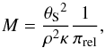 (8)where M is the lens mass and πrel is a proxy to lens distance DL according to Eq. (5). In this equation, ρ is measured from the light curve modelling (Sect. 3.6) and θS is derived below.
To characterise the source, we use a DoPHOT-based data reduction (Schechter et al. 1993) of Danish I and V data to build an instrumental (I,(V − I)) CMD (Fig. 4). Fitting the I-band data for the best-fit model parameters provides IS,DK = 19.85 ± 0.01. We use the RCG method to measure the interstellar extinction. Red clump giant stars are found to be relatively sparse, which makes it difficult to locate precisely the mean instrumental RCG position, (IRCG,DK,(V − I)RCG,DK). To overcome this problem, we cross-calibrate the Danish CMD with a CMD obtained at CTIO in a very similar I filter, by cross-identifying a few clump stars. We then measure IRCG,DK = 15.09 and (V − I)RCG,DK = 0.11. The values of MI,RCG = −0.12 ± 0.09 and (V − I)RCG,0 = 1.06 ± 0.12 are taken from Nataf et al. (2013) at the coordinates of MOA-2007-BLG-197. Measuring the dereddened apparent magnitude of the red clump stars located in the Galactic bulge, Nataf et al. (2013) found a distance to the Galactic centre DGC = 8.20 kpc and an angle between the Galactic bar and the line of sight from the Sun φ = 40°. From these values, the distance to the RCG is 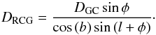 (9)For the Galactic coordinates of MOA-2007-BLG-197, the RCG is in the far side of the bar at a distance DRCG = 8.29 kpc. We adopt a source at the same distance, corresponding to a distance modulus of μ = 14.6 ± 0.3 mag, where the error bars also account for the uncertainty in the position of the RCG.
We then calculate IS,0 = IS,DK + MI,RCG + μ − IRCG,DK and obtain IS,0 = 19.24 ± 0.31, which gives an absolute magnitude of MI = 4.65 ± 0.31. We use a 10 Gyr and solar metallicity isochrone from Bressan et al. (2012) to get the corresponding absolute magnitude MV of the source from which we derive an intrinsic source colour of (V − I)S,0 = 0.88 ± 0.1. This value can be compared to an independent estimate of the source colour based on the method of Gould et al. (2010a). MOA RM-band images are reduced with DoPHOT, and stars are cross-matched between Danish I, V and MOA RM frames (lower panel of Fig. 4). We obtain  (10)where IS,MOA = 20.76 ± 0.02 from the fit of the RM light curve using the best-fit parameters. Hence, IS,DK − IS,MOA = −0.91 ± 0.02, which yields (V − I)S,DK = −0.18 ± 0.10. It follows that the estimated de-reddened source colour is (V − I)S,0 = (V − I)S,DK + (V − I)RCG − (V − I)RCG,DK = 0.77 ± 0.2, which is in good agreement with the previous estimate. In the following, we adopt (V − I)S,0 = 0.88 ± 0.1 (most robust estimate) and IS,0 = 19.24 ± 0.31. The source is thus a G6-K0 Main Sequence star.
From Kervella & Fouqué (2008) brightness-colour relations, we estimate the angular radius of the source,  (11)which yields θS = 0.54 ± 0.05 μas. With a source at DS = 8.3 kpc, the physical source radius is RS = DSθS = 0.96 R⊙. From Carroll & Ostlie (2006), this radius is that of G8 Main Sequence star, which is in very good agreement with the constraint from the colour.
The lens mass-distance relation obtained from Eq. (8) where θS = 0.54 μas and ρ = 5.30 × 10⁻⁴ is plotted in Fig. 6.
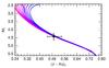 |
Fig. 5 Colour–magnitude diagram (MJ,(J − Ks)0) of the lens. The curves are a set of isochrones from 2 Gyr (in pink) to 8 Gyr (in blue) with solar metallicity (Bressan et al. 2012). The black cross indicates the range of colours and magnitudes explored by the MCMC at the 1σ level. |
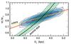 |
Fig. 6 Lens mass-distance relations derived from the source size ρ (1σ around the best value shown by the green shadow limited by the dashed lines) and NaCo (J,H,Ks) colours constrains (respectively yellow, orange, red from top to bottom below the label “colours”). The blue contours (1−4σ) represent the joint posterior probability density P(M,DL) from the MCMC run. |
4.2. Mass-distance relation from NaCo data
Calibrated (J,H,Ks) NaCo magnitudes (Sect. 2.3) provide independently from Eq. (8) further lens mass-distance relations (written below for J only) through  (12)where mJ(L) is the lens apparent reddened magnitude of the lens, AJ the interstellar absorption (given in Sect. 2.3), and MJ the lens absolute magnitude (which is a function of its mass M). The source (J,H,Ks) magnitudes are expressed as (e.g., for J)
  (13)where A = 1.3 is the magnification of the source at the time of the NaCo observations, and assuming that the absorption mostly occurs in the first kiloparsecs towards the bulge. The resulting (J,H,Ks) magnitudes are then computed from the previous equations.
The absolute magnitudes MJ,H,Ks are computed using the isochrones by Bressan et al. (2012) for both the source and lens. For the source we use the same isochrone as in Sect. 4.1. For the lens, we assume an age of 2.5 Gyr and solar metallicity. In fact, as seen in Fig. 5, the lens lies in a region of the isochrones where the age has only very small impact on the magnitudes. The choice of metallicity has slightly more impact, but keeps the variation lower than the magnitude error bars for metallicity changes as large as Z⊙ ± 0.02.
We then use a MCMC algorithm (Sect. 4.4) to match the observed NaCo magnitudes listed in Table 2 (Epoch 1) to the theoretical magnitudes, using the lens mass M and distance DL as fitting parameters. The observed magnitudes serve as Gaussian prior distributions with standard deviation equal to the magnitudes error bars; they are shown as filled curves in Fig. 7. In the same figure, posterior distributions for the resulting magnitudes (lens, and source+lens) are shown in solid and dashed lines respectively. The final lens mass-distance relations are plotted in Fig. 6. It can be seen that while in principle three relations are obtained, they are very strongly correlated and thus only correspond to one effective independent mass-distance relation.
4.3. Mass-distance relation from parallax or orbital motion
In principle, when parallax is measured, a further independent lens mass-distance relation can be obtained by combining Eq. (7) with Eq. (6),  (14)where πE is derived from the light curve modelling. Nevertheless, as discussed in Sect. 3.6, the parallax is degenerate with the lens orbital motion, which prevent us from using this constraint. We however plot on Fig. 6 the typical behaviour of the mass-distance relation obtained from parallax measurements, if πE had been measured. We discuss this problem further below.
4.4. Combination of the constraints and physical parameters
We combined the different mass-distance relations discussed in the previous sections (and shown in Fig. 6) in a MCMC minimisation process to recover the lens mass M and the observer-lens distance DL. We use the measurement and error bars for ρ, (J,H,Ks) and πE to build up Gaussian priors for the Bayesian analysis, and flat (uninformative) priors for M and DL. The values of the parameters correspond to the solution u0> 0, as discussed in Sect. 3.6. We used the convergence criterion of Geweke (1992) to stop the MCMC and compute the posterior probability densities.
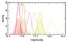 |
Fig. 7 Probability densities of NaCo (J,H,Ks) magnitudes, not corrected for interstellar extinction. Filled curves are Bayesian Gaussian priors based on the NaCo measurements, which are compared to posterior distributions (solid lines). The dotted posterior distributions are those of the lens magnitudes alone (i.e., disentangled from the source; respectivement J,H,Ks from the right to the left). |
As seen in Fig. 6, in principle this problem is over-constrained, with three relations for only two fitting parameters. This enabled us to check the consistency of the different measurements, and investigate further the degeneracy between parallax and lens orbital motion, which prevents πE from being used as a constraint. We first noticed a clear discrepancy between the value of πE derived from the fit (the prior) and the posterior value. This pointed out a strong tension between the three constraints from parallax, source size and infrared colours. We then successively removed the parallax, source size or colours constraints from the MCMC runs. Without the source size constraint, a model with parallax values as large as πE ~ 1.1 was found. This would require a much closer lens (DL ~ 0.6 kpc), a longer Einstein radius (θE ~ 1.6 mas) and consequently a much smaller source size (ρ ~ 3.3 × 10⁻⁴). This value of ρ is many sigma away from that measured from the light curve modelling. Such a difference is very unlikely given the very strong constraint on ρ obtained from the caustic exit modelling. This therefore confirmed previous concerns that in this case, the degeneracy between parallax and lens orbital motion does not allow us to use the parallax mass-distance relation. Consequently, the parallax constraints are removed from the MCMC to derived the final values for M and DL, thus constrained by the source size and the colours.
The final values for M and DL are given in Table 4, with the correlation plot shown in Fig. 6. We also compute the mass of the lens companion, mBD = qM, and find mBD = 41 ± 2 MJ. The host mass is 0.82 ± 0.04 M⊙. The companion is thus a brown dwarf orbiting a solar-type star.
Physical parameters of MOA-2007-BLG-197L and its companion.
We finally perform additional consistency checks on the overall parameters of MOA-2007-BLG-197L. First, we compute the projected lens-source relative velocity 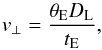 (15)and find v⊥ ≃ 80 km s-1, which is in very good agreement with probability densities predicted by Dominik (2006) for the derived values of tE and DL. Moreover and as a supplementary check, we computed the probability distribution of πE from the distributions of M and DL using Eq. (14), and derived its maximum a posteriori (MAP) value. We then ran again the light curve modelling with this value of πE kept fixed. For the overall consistency, all the parameters are fixed as well, except ṡ and
  (values are given in Table 3, model with u0> 0) which yields the value of the orbital motion parameter γ (see Table 4). From this, we compute
 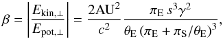 (16)the ratio of the apparent kinetic to potential energy for the binary lens orbit projected onto the plane of the sky (An et al. 2002). Gravitationally bound systems should exhibit 0 <β< 1 (for face-on circular orbits, β = 0.5). Using πS = AU /DS, we find β ≃ 0.08, which is a value consistent with a bound system. In contrast, high parallax values of e.g., πE = 1.1 lead to much lower values of β ≃ 4.5 × 10⁻³. As argued by Batista et al. (2011), a scenario with β ≪ 1 would require highly improbable orbital parameters or projections, such as a very close-in companion seen on a nearly edge-on circular orbit, which is excluded here.
5. MOA-2007-BLG-197Lb in the brown dwarf landscape
While around 1900 exoplanets have been detected so far6, less than a hundred brown dwarfs orbiting stars are known today. The lack of brown dwarf companions to solar-type stars was noticed early after the first exoplanets detections, and referred to as a “brown dwarf desert”. Using the radial velocity method, Marcy & Butler (2000) noted that at tight orbital separations (a< 3AU), companions more massive than 8 MJ represented only a very low fraction of the detected objects. This was not expected from the relatively high frequency (~13%) of binary stars found earlier by Duquennoy & Mayor (1991), also at close separation.
This lack of brown dwarf companions compared to planetary companions has since been confirmed by all detection methods. For instance, Lafrenière et al. (2007) found a frequency of  for 13−75 MJ companions located in the range 25−250 AU from the Gemini Deep Planet Survey. Similarly, Metchev & Hillenbrand (2009) derived a frequency of 3.2 ± 3.1% for brown dwarfs orbiting young solar-type stars in the range 28−1590 AU using adaptive optics direct imaging. McCarthy & Zuckerman (2004) also found a higher proportion of stellar compared to substellar companions to stars, and derived a frequency ratio of ~3−10 at wide separations. Luhman et al. (2007) found that this ratio is comparable to the relative abundance of stars to substellar objects when they are found single, either in star forming regions or in the solar neighbourhood.
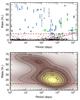 |
Fig. 8 Upper panel: mass-period diagram with brown dwarfs companions detected through radial velocity, transit and direct imaging (blue filled circles for measured masses, and open circles for minimum masses; list adapted from Ma & Ge 2014), and microlensing (green diamonds). For reference, exoplanets detected so far are also displayed (small black circles, http://exoplanets.org). The red dotted line indicates the global radial velocity completeness limit, while the red dashed line marks the region above which data are included to perform the non-parametric, two-dimensional probability density distribution shown in the lower panel. |
The upper panel of Fig. 8 is a mass vs. period diagram which diplays the known brown dwarf companions of solar-type stars detected through microlensing, radial velocimetry, transit and direct imaging. For radial velocimetry and transit, we included objects from Ma & Ge (2014) catalogue with (minimum) masses in the range 13−74 MJ and orbital periods below 2 × 10⁴ d. Furthermore, we have excluded objects with mass uncertainties above 25 MJ, and deleted (false positive) TYC 1240-945-1. Microlensing brown dwarfs are shown as green points, they are: MOA-2011-BLG-149 and OGLE-2011-BLG-0172/MOA-2011-BLG-104 (Shin et al. 2012b), MOA-2010-BLG-073 (Street et al. 2013), OGLE-2013-BLG-0578 (Park et al. 2015) as well as MOA-2007-BLG-197 (this paper). For consistency with Doppler and transit data, we did not include MOA-2009-BLG-411 (Bachelet et al. 2012) which has a large uncertainty in the mass. In the case of microlensing objects for which only projected separations a⊥ were measured (all objects in this case), we estimate the (physical) semi-major axis a as the median of the probability distribution of Gould & Loeb (1992), which we find to be equal to  . Kepler’s third law is then used to yield the estimated period. The error bar on measured a⊥ is propagated to a following the previous equation, and the error bar on the period is obtained through a MCMC run including uncertainties on a and primary mass M (Gaussian distributions are assumed).
As seen in Fig. 8, the distribution of brown dwarfs is not uniform, in particular it exhibits an increasing frequency of objects with increasing orbital period. Furthermore, Ma & Ge (2014) argue that the driest part of the brown dwarf desert seems to be confined within a region at close separation, namely within P< 100 d and for masses within 30−55 MJ for Sun-like host stars. They subsequently split the objects into two distinct populations, whether their mass is higher or lower than 42.5 MJ: the more massive brown dwarfs would mainly be the outcome of gravitational fragmentation and collapse of a molecular cloud (star-like formation scenario, corroborated by an eccentricity distribution similar to binary stars), while brown dwarfs below 42.5 MJ would mainly result from gravitational instability within the proto-planetary disk. But other authors such as Guillot et al. (2012), however, argue that the depletion of objects at tight orbits may as well be explained by a loss of an initial population of close-in brown dwarfs due to tidal interactions with their host stars. In this scenario, close-in, massive objects lose angular momentum due to the slower rotation of the star relative to the planets orbital motion, spiral in and fall into the star. This effect is predicted to peak for G-dwarf primaries and should not be important for earlier-type stars, which is supported by the detection of close-in brown dwarfs around F-type stars.
Different mechanisms may overlap to shape the brown dwarfs landscape, and lead to a more complex structure than previously discussed. To analyse it further, we performed a non-parametric, two-dimensional probability density distribution fit to the data, only for objects above the red dashed line (i.e., above the radial velocity completeness limit, based on Mayor et al. 2011, and marked by the red dotted line in Fig. 8). The probability density estimation is based on Scott (1992); in practice we used a Gaussian kernel, and follow Silverman (1986) rule to estimate the bandwidth parameter. The resulting probability density is shown in the lower panel of Fig. 8. We used two different methods to compute the bandwidth parameter, Silverman (1986) or Scott (1992), and found that the resulting probability density is relatively stable, even if a few data points are removed from sparsely sampled regions.
The first striking feature of the density profile (lower panel of Fig. 8) is a region of depletion of objects at intermediate masses (M ~ 30−60 MJ) and short orbital periods (P ≲ 30 d). This matches the region referred to as the driest part of the brown dwarf desert according to Ma & Ge (2014). Second, an accumulation of objects can be seen around P ~ 500 d and M ~ 20 MJ (following the apparent trend observed for giant planets, black data points in Fig. 8). Third, we find another depletion of objects at long orbital periods (P ≳ 500 d) and high masses (M ≳ 50 MJ). Since the brown dwarf sample is drawn from various surveys (mainly from radial velocities), the interpretation of these features should be taken with caution. Although all brown dwarfs in Fig. 8 are chosen above the radial velocity completeness limit from Mayor et al. (2011), it is not guaranteed that these objects are not affected by observational biases. In particular, a degeneracy between mass and period is increasingly affecting very long-period brown dwarfs, and the different surveys should be corrected from their sample size. Hence, while a thorough analysis of all these factors is necessary to assess the exact shape of the brown dwarfs distribution, the gross features emerging from the lower panel of Fig. 8 may well be real. If we split the density profile into two regions of masses above and below 42.5 MJ as discussed by Ma & Ge (2014), the distribution of high-mass objects can be seen as shifted towards shorts orbital periods (P ~ 30 d), while less massive objects appear to pile up at longer orbital periods (P ~ 500 d). This supports the claim of Ma & Ge (2014) that massive objects would accumulate at short periods as a result of gravitational collapse of a molecular cloud, contrary to less-massive objects built up by gravitational instability in the disk which would accumulate at longer periods. Nevertheless, the depletion at intermediate masses and short periods would as well be affected by a star-engulfing mechanism advocated by Guillot et al. (2012), in particular because almost all brown dwarfs included here orbit Sun-like stars, for which this effect peaks.
The distribution of brown dwarfs as a function of mass and period still remains uncertain because of a lack of detections. It is thus difficult to distinguish between the different mechanisms which shape the brown dwarf desert. Moreover, these detections are mostly objects orbiting Sun-like stars, which makes it difficult to study their distribution as a function of host star mass. While the MOA-2007-BLG-197L companion orbits a G-K dwarf host, microlensing hosts are most frequently M-K dwarfs. Hence, future microlensing surveys will provide unique information on the brown dwarf distribution for low-mass hosts, thus offering a complementary mass bin to other methods.
6. Summary and prospects
We have presented MOA-2007-BLG-197Lb, the first brown dwarf discovered around a Sun-like star through gravitational microlensing. The system is located at  from the Earth, the brown dwarf companion has a mass of 41 ± 2 MJ and was observed at a projected distance of 4.3 ± 0.1 AU from a K dwarf host star. We have performed a non-parametric probability density distribution fit to the population of brown dwarf companions detected so far. The resulting density profile has a complex structure, leading to a brown dwarf landscape most likely shaped by different (and perhaps competitive) formation or destruction mechanisms. While it seems difficult with the current data set to distinguish observationally which are the dominant mechanisms, an answer to this question appears to within the reach of further observations in the near to mid-term future.
Gravitational microlensing is an exceptional tool to detect brown dwarfs as free-floating objects, companions to stars or as brown dwarfs binaries. It has a unique sensitivity to detect brown dwarfs companions to stars of any type, in particular at long orbital periods. Recent advances in using networks of robotic telescopes (e.g., Tsapras et al. 2009) will provide in a near future an order of magnitudes more brown dwarfs detections through microlensing. Future microlensing space missions (Penny et al. 2013; Yee et al. 2014; Beaulieu et al. 2010) also carry important promises for providing unique information on the populations of brown dwarfs in their different configurations.
Online material
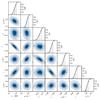 |
Fig. 9 Correlations between the parameters derived from ESBL’s model discussed in Sect. 3.1. The red point refers to the best-fitting model obtained. |
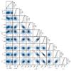 |
Fig. 10 Idem for ESBL+P’s model. |
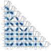 |
Fig. 11 Idem for ESBL+LOM’s model. |
 |
Fig. 12 Idem for ESBL+P+LOM’s model (u0> 0) with ρ′ = 5.3 × 10⁻⁴. |
THJD = HJD−2 450 000.
ESO Programme ID 279.C-5044(A).
ESO Programme ID 381.C-0425(A).
Note that the difference in the transmission profile between K and Ks bands is less than 1%, so negligible in the present case.
These very intensive computations were performed on the Tasmanian cluster TPAC (Tasmanian Partnership for Advanced Computing).
Acknowledgments
A.C. acknowledges financial support from the Emergence UPMC 2012 grant. C.R. and A.C. are grateful to Bo Ma for providing us with the brown dwarfs catalogue used in Ma & Ge (2014). We especially thank the University of Tasmania for granting us access to their TPAC supercomputer facilities where part of the calculations were carried out. Work by C.H. was supported by Creative Research Initiative Program (2009-0081561) of National Research Foundation of Korea. K.H., M.D. and M.H. are supported by NPRP grant NPRP-09-476-1-78 from the Qatar National Research Fund (a member of Qatar Foundation). M.H. acknowledges support from the Villum foundation. S.D. is supported by “the Strategic Priority Research Program- The Emergence of Cosmological Structures” of the Chinese Academy of Sciences (grant No. XDB09000000).
References
- Alard, C. 2000, A&AS, 144, 363 [NASA ADS] [CrossRef] [EDP Sciences] [Google Scholar]
- Alard, C., & Lupton, R. H. 1998, ApJ, 503, 325 [NASA ADS] [CrossRef] [Google Scholar]
- Albrow, M. D., Beaulieu, J.-P., Caldwell, J. A. R., et al. 1999a, ApJ, 522, 1022 [NASA ADS] [CrossRef] [Google Scholar]
- Albrow, M. D., Beaulieu, J.-P., Caldwell, J. A. R., et al. 1999b, ApJ, 522, 1011 [NASA ADS] [CrossRef] [Google Scholar]
- Albrow, M. D., Horne, K., Bramich, D. M., et al. 2009, MNRAS, 397, 2099 [NASA ADS] [CrossRef] [Google Scholar]
- An, J. H., Albrow, M. D., Beaulieu, J.-P., et al. 2002, ApJ, 572, 521 [NASA ADS] [CrossRef] [Google Scholar]
- Bachelet, E., Fouqué, P., Han, C., et al. 2012, A&A, 547, A55 [NASA ADS] [CrossRef] [EDP Sciences] [Google Scholar]
- Batista, V., Gould, A., Dieters, S., et al. 2011, A&A, 529, A102 [NASA ADS] [CrossRef] [EDP Sciences] [Google Scholar]
- Beaulieu, J. P., Bennett, D. P., Batista, V., et al. 2010, in Pathways Towards Habitable Planets, eds. V. Coudé du Foresto, D. M. Gelino, & I. Ribas, ASP Conf. Ser., 430, 266 [Google Scholar]
- Bennett, D. P. 2010, ApJ, 716, 1408 [NASA ADS] [CrossRef] [Google Scholar]
- Bonfils, X., Delfosse, X., Udry, S., et al. 2013, A&A, 549, A109 [NASA ADS] [CrossRef] [EDP Sciences] [Google Scholar]
- Bozza, V. 2010, MNRAS, 408, 2188 [NASA ADS] [CrossRef] [Google Scholar]
- Bozza, V., Dominik, M., Rattenbury, N. J., et al. 2012, MNRAS, 424, 902 [NASA ADS] [CrossRef] [Google Scholar]
- Bressan, A., Marigo, P., Girardi, L., et al. 2012, MNRAS, 427, 127 [NASA ADS] [CrossRef] [Google Scholar]
- Burrows, A., Hubbard, W. B., Lunine, J. I., & Liebert, J. 2001, Rev. Mod. Phys., 73, 719 [Google Scholar]
- Carroll, B. W., & Ostlie, D. A. 2006, An introduction to modern astrophysics and cosmology (Addison-Wesley) [Google Scholar]
- Cassan, A. 2008, A&A, 491, 587 [NASA ADS] [CrossRef] [EDP Sciences] [Google Scholar]
- Cassan, A., Beaulieu, J. P., Brillant, S., et al. 2004, A&A, 419, L1 [NASA ADS] [CrossRef] [EDP Sciences] [Google Scholar]
- Cassan, A., Beaulieu, J.-P., Fouqué, P., et al. 2006, A&A, 460, 277 [NASA ADS] [CrossRef] [EDP Sciences] [Google Scholar]
- Cassan, A., Horne, K., Kains, N., Tsapras, Y., & Browne, P. 2010, A&A, 515, A52 [NASA ADS] [CrossRef] [EDP Sciences] [Google Scholar]
- Cassan, A., Kubas, D., Beaulieu, J.-P., et al. 2012, Nature, 481, 167 [NASA ADS] [CrossRef] [Google Scholar]
- Choi, J.-Y., Han, C., Udalski, A., et al. 2013, ApJ, 768, 129 [NASA ADS] [CrossRef] [Google Scholar]
- Claret, A., & Bloemen, S. 2011, A&A, 529, A75 [NASA ADS] [CrossRef] [EDP Sciences] [Google Scholar]
- Deleuil, M., Deeg, H. J., Alonso, R., et al. 2008, A&A, 491, 889 [NASA ADS] [CrossRef] [EDP Sciences] [Google Scholar]
- Devillard, N. 1999, in Astronomical Data Analysis Software and Systems VIII, eds. D. M. Mehringer, R. L. Plante, & D. A. Roberts, ASP Conf. Ser., 172, 333 [Google Scholar]
- Díaz, R. F., Damiani, C., Deleuil, M., et al. 2013, A&A, 551, L9 [NASA ADS] [CrossRef] [EDP Sciences] [Google Scholar]
- Diolaiti, E., Bendinelli, O., Bonaccini, D., et al. 2000, in Adaptive Optical Systems Technology, ed. P. L. Wizinowich, Proc. SPIE, 4007, 879 [Google Scholar]
- Dominik, M. 2006, MNRAS, 367, 669 [NASA ADS] [CrossRef] [Google Scholar]
- Dominik, M. 2007, MNRAS, 377, 1679 [NASA ADS] [CrossRef] [Google Scholar]
- Dong, S., DePoy, D. L., Gaudi, B. S., et al. 2006, ApJ, 642, 842 [NASA ADS] [CrossRef] [Google Scholar]
- Dong, S., Bond, I. A., Gould, A., et al. 2009, ApJ, 698, 1826 [NASA ADS] [CrossRef] [Google Scholar]
- Duquennoy, A., & Mayor, M. 1991, A&A, 248, 485 [NASA ADS] [Google Scholar]
- Geweke, J. 1992, in Bayesian Statistics, eds. J. M. Bernardo, J. O. Berger, A. P. Dawid, & A. F. M. Smith (New York: Oxford University Press), 169 [Google Scholar]
- Gould, A. 2004, ApJ, 606, 319 [NASA ADS] [CrossRef] [Google Scholar]
- Gould, A. 2008, ApJ, 681, 1593 [NASA ADS] [CrossRef] [Google Scholar]
- Gould, A., & Gaucherel, C. 1997, ApJ, 477, 580 [NASA ADS] [CrossRef] [Google Scholar]
- Gould, A., & Loeb, A. 1992, ApJ, 396, 104 [NASA ADS] [CrossRef] [Google Scholar]
- Gould, A., Udalski, A., Monard, B., et al. 2009, ApJ, 698, L147 [NASA ADS] [CrossRef] [Google Scholar]
- Gould, A., Dong, S., Bennett, D. P., et al. 2010a, ApJ, 710, 1800 [NASA ADS] [CrossRef] [Google Scholar]
- Gould, A., Dong, S., Gaudi, B. S., et al. 2010b, ApJ, 720, 1073 [NASA ADS] [CrossRef] [Google Scholar]
- Guillot, T., Lin, D. N. C., & Morel, P. 2012, in AAS Meet. Abstr., 220, 121.03 [Google Scholar]
- Han, C., Jung, Y. K., Udalski, A., et al. 2013, ApJ, 778, 38 [NASA ADS] [CrossRef] [Google Scholar]
- Janczak, J., Fukui, A., Dong, S., et al. 2010, ApJ, 711, 731 [NASA ADS] [CrossRef] [Google Scholar]
- Johnson, J. A., Apps, K., Gazak, J. Z., et al. 2011, ApJ, 730, 79 [NASA ADS] [CrossRef] [Google Scholar]
- Jung, Y. K., Udalski, A., Sumi, T., et al. 2015, ApJ, 798, 123 [NASA ADS] [CrossRef] [Google Scholar]
- Kains, N., Cassan, A., Horne, K., et al. 2009, MNRAS, 395, 787 [NASA ADS] [CrossRef] [Google Scholar]
- Kains, N., Browne, P., Horne, K., Hundertmark, M., & Cassan, A. 2012, MNRAS, 426, 2228 [NASA ADS] [CrossRef] [Google Scholar]
- Kato, D., Nagashima, C., Nagayama, T., et al. 2007, PASJ, 59, 615 [NASA ADS] [Google Scholar]
- Kervella, P., & Fouqué, P. 2008, A&A, 491, 855 [NASA ADS] [CrossRef] [EDP Sciences] [Google Scholar]
- Kubas, D., Cassan, A., Beaulieu, J. P., et al. 2005, A&A, 435, 941 [NASA ADS] [CrossRef] [EDP Sciences] [Google Scholar]
- Kubas, D., Beaulieu, J. P., Bennett, D. P., et al. 2012, A&A, 540, A78 [NASA ADS] [CrossRef] [EDP Sciences] [Google Scholar]
- Lafrenière, D., Doyon, R., Marois, C., et al. 2007, ApJ, 670, 1367 [NASA ADS] [CrossRef] [Google Scholar]
- Luhman, K. L., Joergens, V., Lada, C., et al. 2007, Protostars and Planets V, 951, 443 [NASA ADS] [Google Scholar]
- Ma, B., & Ge, J. 2014, MNRAS, 439, 2781 [NASA ADS] [CrossRef] [Google Scholar]
- Mao, S., & Paczynski, B. 1991, ApJ, 374, L37 [NASA ADS] [CrossRef] [Google Scholar]
- Marcy, G. W., & Butler, R. P. 2000, PASP, 112, 137 [NASA ADS] [CrossRef] [Google Scholar]
- Mayor, M., Marmier, M., Lovis, C., et al. 2011, A&A, submitted [arXiv:1109.2497] [Google Scholar]
- McCarthy, C., & Zuckerman, B. 2004, AJ, 127, 2871 [NASA ADS] [CrossRef] [Google Scholar]
- Metchev, S. A., & Hillenbrand, L. A. 2009, ApJS, 181, 62 [NASA ADS] [CrossRef] [Google Scholar]
- Mollière, P., & Mordasini, C. 2012, A&A, 547, A105 [NASA ADS] [CrossRef] [EDP Sciences] [Google Scholar]
- Moutou, C., Bonomo, A. S., Bruno, G., et al. 2013, A&A, 558, L6 [NASA ADS] [CrossRef] [EDP Sciences] [Google Scholar]
- Nataf, D. M., Gould, A., Fouqué, P., et al. 2013, ApJ, 769, 88 [NASA ADS] [CrossRef] [Google Scholar]
- Park, H., Udalski, A., Han, C., et al. 2015, ApJ, 805, 117 [NASA ADS] [CrossRef] [Google Scholar]
- Penny, M. T., Kerins, E., Rattenbury, N., et al. 2013, MNRAS, 434, 2 [NASA ADS] [CrossRef] [Google Scholar]
- Persson, S. E., Murphy, D. C., Krzeminski, W., Roth, M., & Rieke, M. J. 1998, AJ, 116, 2475 [NASA ADS] [CrossRef] [Google Scholar]
- Sahlmann, J., Ségransan, D., Queloz, D., et al. 2011, A&A, 525, A95 [NASA ADS] [CrossRef] [EDP Sciences] [Google Scholar]
- Schechter, P. L., Mateo, M., & Saha, A. 1993, PASP, 105, 1342 [NASA ADS] [CrossRef] [Google Scholar]
- Scott, D. W. 1992, Multivariate Density Estimation: Theory, Practice, and Visualization (New York, Chicester: John Wiley & Sons) [Google Scholar]
- Shin, I.-G., Han, C., Choi, J.-Y., et al. 2012a, ApJ, 755, 91 [NASA ADS] [CrossRef] [Google Scholar]
- Shin, I.-G., Han, C., Gould, A., et al. 2012b, ApJ, 760, 116 [NASA ADS] [CrossRef] [Google Scholar]
- Silverman, B. W. 1986, Density Estimation for Statistics and Data Analysis (London: Chapman and Hall) [Google Scholar]
- Skowron, J., Udalski, A., Gould, A., et al. 2011, ApJ, 738, 87 [NASA ADS] [CrossRef] [Google Scholar]
- Street, R. A., Choi, J.-Y., Tsapras, Y., et al. 2013, ApJ, 763, 67 [NASA ADS] [CrossRef] [Google Scholar]
- Sumi, T., Kamiya, K., Bennett, D. P., et al. 2011, Nature, 473, 349 [NASA ADS] [CrossRef] [PubMed] [Google Scholar]
- Tsapras, Y., et al. 2009, Astron. Nachr., 330, 4 [NASA ADS] [CrossRef] [Google Scholar]
- Yee, J. C., Albrow, M., Barry, R. K., et al. 2014, ArXiv e-prints [arXiv:1409.2759] [Google Scholar]
- Zub, M., Cassan, A., Heyrovský, D., et al. 2011, A&A, 525, A15 [NASA ADS] [CrossRef] [EDP Sciences] [Google Scholar]
All Tables
Derived NaCo magnitudes of the microlensing event target in the (J,H,Ks) filters for the two epochs 2007 August 20/21 (epoch 1) and 2008 August 3/4 (epoch 2).
All Figures
|
Fig. 1 Upper panel: the light curve of MOA-2007-BLG-197 and the best-fit model (solid line) with a zoom on the caustic exit on the right-hand side. On the left-hand side, the structure of the resonant caustic is drawn in red, as well as the trajectory of the source, in black (axes are in Einstein radius units). The source is too small to be distinguished. The four intervals E1−4 indicate time intervals where possible source caustic crossing (caustic entry) have been investigated. Lower panel: the residuals of the best-fit model. |
| In the text | |
|
Fig. 2 Left: sub-region (94″ × 77″) of an original 3′ × 3′Ks-band IRSF image used to calibrate the NaCo magnitudes. Right: corresponding Ks-band NaCo image (27″ × 25″) used to cross-identify the stars. |
| In the text | |
|
Fig. 3 (J,J − Ks) colour–magnitude diagram in the 2MASS system combining NaCo and IRSF data (respectively, in blue and black). The red dot is the magnitude/colour of the source derived from the source characterisation (Sect. 4.1). The values are not corrected for interstellar extinction. The red clump (RCG) is fitted by the red over-plotted 10 Gyr, solar-metallicity isochrone from Bressan et al. (2012). |
| In the text | |
|
Fig. 4 Upper panel: (I,V − I) Danish instrumental CMD of the field around MOA-2007-BLG-197, not corrected for interstellar extinction. The red point marks the position of the RCG. The magnitude of the microlensing target is in blue (i.e. magnified source, lens and blended light). The orange point corresponds to the source alone. Lower panel: empirical linear relation between instrumental colours (IDK − IMOA) and (V − I)DK (red and green points are astrometric matches that are uncrowded in the MOA image; after sigma-clipping, only red points are used for the fit). |
| In the text | |
|
Fig. 5 Colour–magnitude diagram (MJ,(J − Ks)0) of the lens. The curves are a set of isochrones from 2 Gyr (in pink) to 8 Gyr (in blue) with solar metallicity (Bressan et al. 2012). The black cross indicates the range of colours and magnitudes explored by the MCMC at the 1σ level. |
| In the text | |
|
Fig. 6 Lens mass-distance relations derived from the source size ρ (1σ around the best value shown by the green shadow limited by the dashed lines) and NaCo (J,H,Ks) colours constrains (respectively yellow, orange, red from top to bottom below the label “colours”). The blue contours (1−4σ) represent the joint posterior probability density P(M,DL) from the MCMC run. |
| In the text | |
|
Fig. 7 Probability densities of NaCo (J,H,Ks) magnitudes, not corrected for interstellar extinction. Filled curves are Bayesian Gaussian priors based on the NaCo measurements, which are compared to posterior distributions (solid lines). The dotted posterior distributions are those of the lens magnitudes alone (i.e., disentangled from the source; respectivement J,H,Ks from the right to the left). |
| In the text | |
|
Fig. 8 Upper panel: mass-period diagram with brown dwarfs companions detected through radial velocity, transit and direct imaging (blue filled circles for measured masses, and open circles for minimum masses; list adapted from Ma & Ge 2014), and microlensing (green diamonds). For reference, exoplanets detected so far are also displayed (small black circles, http://exoplanets.org). The red dotted line indicates the global radial velocity completeness limit, while the red dashed line marks the region above which data are included to perform the non-parametric, two-dimensional probability density distribution shown in the lower panel. |
| In the text | |
|
Fig. 9 Correlations between the parameters derived from ESBL’s model discussed in Sect. 3.1. The red point refers to the best-fitting model obtained. |
| In the text | |
|
Fig. 10 Idem for ESBL+P’s model. |
| In the text | |
|
Fig. 11 Idem for ESBL+LOM’s model. |
| In the text | |
|
Fig. 12 Idem for ESBL+P+LOM’s model (u0> 0) with ρ′ = 5.3 × 10⁻⁴. |
| In the text | |
Current usage metrics show cumulative count of Article Views (full-text article views including HTML views, PDF and ePub downloads, according to the available data) and Abstracts Views on Vision4Press platform.
Data correspond to usage on the plateform after 2015. The current usage metrics is available 48-96 hours after online publication and is updated daily on week days.
Initial download of the metrics may take a while.