| Issue |
A&A
Volume 580, August 2015
|
|
|---|---|---|
| Article Number | A27 | |
| Number of page(s) | 14 | |
| Section | Stellar structure and evolution | |
| DOI | https://doi.org/10.1051/0004-6361/201425290 | |
| Published online | 22 July 2015 | |
Tight asteroseismic constraints on core overshooting and diffusive mixing in the slowly rotating pulsating B8.3V star KIC 10526294⋆,⋆⋆
1
Institute of Astronomy,
KU Leuven, Celestijnenlaan 200D,
3001
Leuven,
Belgium
e-mail:
This email address is being protected from spambots. You need JavaScript enabled to view it.
2
Department of Astrophysics, IMAPP, Radboud University
Nijmegen, PO Box
9010, 6500 GL
Nijmegen, The
Netherlands
Received: 6 November 2014
Accepted: 22 May 2015
Abstract
Context. KIC 10526294 was recently discovered to be a very slowly rotating and slowly pulsating late B-type star. Its 19 consecutive dipole gravity modes constitute a series with almost constant period spacing. This unique collection of identified modes probes the near-core environment of this star and holds the potential to reveal the size and structure of the overshooting zone above the convective core, as well as the mixing properties of the star.
Aims. We revisit the asteroseismic modelling of this star with specific emphasis on the properties of the core overshooting, while considering additional diffusive mixing throughout the radiative envelope of the star.
Methods. We pursued forward seismic modelling based on adiabatic eigenfrequencies of equilibrium models for eight extensive evolutionary grids tuned to KIC 10526294 by varying the initial mass, metallicity, chemical mixture, and the extent of the overshooting layer on top of the convective core. We examined models for both OP and OPAL opacities and tested the occurrence of extra diffusive mixing throughout the radiative interior.
Results. We find a tight mass-metallicity relation within the ranges M ∈ [ 3.13,3.25 ] M⊙ and Z ∈ [ 0.014,0.028 ]. We deduce that an exponentially decaying diffusive core overshooting prescription describes the seismic data better than a step function formulation and derive a value of fov between 0.017 and 0.018. Moreover, the inclusion of extra diffusive mixing with a value of log Dmix between 1.75 and 2.00 dex (with Dmix in cm2 s-1) improves the goodness-of-fit based on the observed and modelled frequencies by a factor ~11 compared to the case where no extra mixing is considered, irrespective of the (M,Z) combination within the allowed seismic range.
Conclusions. The inclusion of diffusive mixing in addition to core overshooting is essential to explain the structure in the observed period spacing pattern of this star. Moreover, for the input physics and chemical mixtures we investigated, we deduce that an exponentially decaying prescription for the core overshooting is to be preferred over a step function, regardless of the adopted mixture or choice of opacity tables. Our best models for KIC 10526294 approach the seismic data to a level that they can serve future inversion of its stellar structure.
Key words: asteroseismology / stars: oscillations / stars: interiors / stars: evolution / stars: individual: KIC 10526294 / opacity
The MESA inlists, the extended opacity tables, and the best five representative GYRE models in Tables 3, and 4 are available at the CDS via anonymous ftp to cdsarc.u-strasbg.fr (130.79.128.5) or via http://cdsarc.u-strasbg.fr/viz-bin/qcat?J/A+A/580/A27
Appendices are available in electronic form at http://www.aanda.org
Postdoctoral Fellow at KU Leuven funded by the Belgian Federal Science Policy Office (BELSPO).
Postdoctoral Fellow of the Fund for Scientific Research (FWO), Flanders, Belgium.
© ESO, 2015
1. Introduction
Intermediate and massive (M ≳ 2.5M⊙) main-sequence (MS) stars of spectral type OB harbour a fully developed convective core below a radiative envelope during their core hydrogen-burning phase. As their MS evolution progresses, the decrease in the central hydrogen content Xc implies that the convective core shrinks and it hence leaves behind a chemical gradient ∇μ of CNO-processed material at the interface between the inner convective core and the outer radiative envelope. The extent of this interface zone and its mixing properties remain largely unknown. Asteroseismology in principle offers the opportunity to probe this zone.
Stars are multi-component fluids, consisting of chemical species i with a mass fraction denoted as Xi. The spatial abundance distribution Xi(r,t) does not stay constant during the evolution. In burning regions, thermonuclear reactions provide a balance between the depletion of the elements i that are burnt and the production of heavier elements, while the chemical mixture stays intact in the envelope. In the absence of rotation and in a diffusive approximation, the spatial and temporal change of the individual mass fractions Xi are governed by the following transport equation in the Lagrangian description (e.g. Heger et al. 2000): ![Mathematical equation: \begin{equation} \label{e-Xi} \frac{{\rm d}X_i}{{\rm d}t} = \left(\frac{{\rm d}X_i}{{\rm d}t}\right)_{\rm nuc} + \frac{\partial }{\partial m}\left[(4\pi r^2\rho)^2 \, D_{\rm mix} \, \left( \frac{\partial X_i}{\partial m} \right)_t \right], \end{equation}](/articles/aa/full_html/2015/08/aa25290-14/aa25290-14-eq17.png) (1)where the first term accounts for the changes induced by nuclear burning, while the second term accounts for the mixing of element i according to its spatial gradient ∂Xi/∂m. In this equation, Dmix is the effective diffusive mixing coefficient, which has a unit of area over time (e.g. Maeder 2009). Advective phenomena such as meridional circulation are excluded in this formulation. Equation (1) is solved subject to boundary conditions for the abundance gradients in the core and at the surface, that is, (∂Xi/∂m)core = (∂Xi/∂m)surface = 0.
(1)where the first term accounts for the changes induced by nuclear burning, while the second term accounts for the mixing of element i according to its spatial gradient ∂Xi/∂m. In this equation, Dmix is the effective diffusive mixing coefficient, which has a unit of area over time (e.g. Maeder 2009). Advective phenomena such as meridional circulation are excluded in this formulation. Equation (1) is solved subject to boundary conditions for the abundance gradients in the core and at the surface, that is, (∂Xi/∂m)core = (∂Xi/∂m)surface = 0.
A collection of mechanisms contributes to the local mixing in the stellar interior. Convection is the dominant one, because it homogenises convective zones on a dynamical timescale, which is very short compared to the nuclear timescale. Mixing in the radiative interior occurs on a much longer timescale. A handful of mixing mechanisms that can operate in the stellar envelope have been proposed, such as core convective overshooting (Saslaw & Schwarzschild 1965; Roxburgh 1965; Shaviv & Salpeter 1973), semi-convective mixing (Schwarzschild & Härm 1958; Kato 1966; Langer et al. 1983), rotational mixing (Weiss et al. 1988; Charbonnel et al. 1992; Chaboyer 1994), shear-induced mixing (Jeans 1928; Zahn 1992), and mixing induced by internal magnetic fields (Heger et al. 2005). Following a multivariate analysis of the seismic, magnetic, and rotational properties of a sample of slowly rotating Galactic OB-type stars, Aerts et al. (2014) found the observational evidence for pulsationally induced mixing to be stronger than for rotational mixing.
In the computation of stellar evolution models, most of these mixing mechanisms are effectively defined in a diffusion approximation and described by a diffusion coefficient (e.g. Heger et al. 2000). In the absence of quantitative observational constraints on the individual contributions for each of the mixing mechanisms, their net effect Dmix is either linearly summed up (Heger et al. 2000, 2005) or their interaction is considered (Maeder et al. 2013; Ding & Li 2014). In this paper, Dmix in radiative interior is a linear superposition of individual mixing processes. Any local modification to the shape of the mixing profile Dmix(r) propagates into the stellar structure through Eq. (1) and subsequently influences the shape of the Brunt-Väisälä frequency, which incorporates the gradient of the mean molecular weight. Given the sensitivity of high-order g-modes to the detailed shape of the Brunt-Väisälä frequency, their frequencies are influenced by the local shape of Dmix(r). For this reason, and thanks to asteroseismology based on the high-precision Kepler space-based photometry, we are able to investigate whether observational constraints on Dmix are within reach.
Before high-precision space photometry was available, Miglio et al. (2008) have already shown how varying Dmix influences the morphology of the period spacings of gravity modes in MS stars with convective cores. Degroote et al. (2010) applied this approach to model the detected period spacing of the slowly rotating pulsating B3V star HD 50230 observed with the CoRoT mission for five months. They assumed the detected sequence of consecutive modes belongs to the dipole (ℓ = 1) series. They concluded that HD 50230 has a mass between 7 and 8 M⊙, has consumed some 60% of its initial hydrogen, and required a value of log Dmix between 3.48 and 4.30 cm2 s-1 to explain the small periodic deviation of 240 s from a constant period spacing of 9418 s for an assumed value of 0.02 for the metallicity. However, this result was criticised by Szewczuk et al. (2014), who suggested that some of the low-amplitude peaks in the series might be due to modes of higher degree.
KIC 10526294 was recently discovered to be a very slowly rotating and slowly pulsating B (SPB) star from Kepler photometry (Pápics et al. 2014, hereafter P14), exhibiting 19 rotationally split dipole gravity modes. Pápics and collaborators performed forward seismic modelling and considered core overshooting in the diffusive exponentially decaying prescription defined in Freytag et al. (1996) and Herwig (2000). We designate the free parameter of this prescription as fov (and discuss it in Eq. (3) below). But, they only succeeded to put an upper limit on this free parameter: fov ≲ 0.015.
In contrast to the case of HD 50230, there is no doubt about the identification of the degree of the modes for KIC 10526294. Hence, we here revisit the forward modelling of this SPB (Sect. 2) and introduce two improvements. The first one concerns the inclusion of realistic frequency uncertainties, to compute reduced χ2 values as a means of the model selection criterion. P14 only adopted a first rough goodness-of-fit procedure for the model selection, denoted here as  . This goodness-of-fit was based on the conservative Rayleigh limit of 0.000685 d-1 for the frequency error of all 19 detected modes, with the argument that the uncertainties on theoretical predictions of oscillation frequencies of pulsating B stars are typically about 0.001 d-1 (Briquet et al. 2007). That was adequate for their modelling, because they only compared models with one set of input physics and with one fixed number of degrees of freedom. Since we here compare models with and without extra diffusive mixing, and thus with a different number of degrees of freedom, we must use a more appropriate statistical description to perform the model selection. This requires the determination of individual frequency uncertainties, as explained in Sect. 2. The second improvement concerns a more detailed model comparison, where we consider different elements of the input physics, such as opacities, chemical mixtures and two different descriptions for the core overshooting. Moreover, we add models based on the inclusion of extra diffusive mixing outside the convective and overshooting zones, described by a coefficient Dmix.
We introduce the target star in Sect. 2 and explain how we took into account its seismic data in Sect. 3. The physical ingredients of the evolutionary models computed with the MESA code (Paxton et al. 2011, 2013, version 5548) are explained in Sect. 4. The adiabatic zonal dipole frequencies for each input model along the evolutionary tracks were computed with the GYRE pulsation code (Townsend & Teitler 2013, version 3.0). In Sect. 5, we explain the model selection based on a reduced χ2 method. The results of our grid search to select the best models to explain the seismic data of KIC 10526294 are reported in Sect. 5. Our consideration of three metal mixtures and both OP and OPAL opacities is exploited in terms of the mode stability for the best models in Sect. 6. Finally, we discuss our results in Sect. 7.
2. The showcase of KIC 10526294
P14 identified KIC 10526294 as a new SPB star (e.g. Waelkens 1991; De Cat & Aerts 2002, for a definition) from its Kepler light curve, which has a duration of ΔT = 1460 d. Its effective temperature, surface gravity, and metallicity were determined by P14 from high-resolution spectroscopy: Teff = 11 500 ± 500 K, log g = 4.1 ± 0.2 dex, and  . P14 performed a full study of the Kepler photometry and identified 19 consecutive dipole ℓ = 1g-mode triplets. As mentioned above, we consider these 19 zonal-mode frequencies with their appropriate errors. The latter were determined following the methodology discussed in detail in Degroote et al. (2009), which is based on the theory of time-series analysis of correlated data by Schwarzenberg-Czerny (1991). In practice this implies taking the formal errors of the non-linear least-squares fit to the light curve and to correct them for the signal-to-noise ratio, sampling, and correlated nature of the data. Applying the procedure discussed in Degroote et al. (2009) to KIC 10526294 results in a correction factor of 3.0 to be applied to the formal errors listed in Table B.1 in P14. For convenience, we repeat the 19 zonal dipole frequencies, their periods and period spacings and their corresponding 1σ errors in Table 1.
As discussed in P14, the average rotational frequency splitting for the m = ± 1 components of the dipole modes points to a rotation period of ~188 d when averaged over the entire depth of the star, implying that KIC 10526294 is an ultra-slow rotator. According to the survey of galactic B stars by Huang et al. (2010), the probability of finding a very slowly rotating late B-type star (2 ≤ M/M⊙ ≤ 4) is low (their Fig. 7a). Thus, KIC 10526294 is optimally suited to study mixing mechanisms for a case where the effect of rotation is negligible.
Based on the initial asteroseismic modelling presented in P14, the mass of KIC 10526294 is roughly 3.2 M⊙, and the star is situated very close to the ZAMS. P14 assumed convective core overshooting and semi-convective mixing (according to the prescription by Langer et al. 1983, with αsc = 10-2). They found their best seismic models (their Table 6) to have a core overshooting fov in the range from zero to 0.015. In what follows, we start from the same grid of models as in P14 but consider additional extra mixing, various chemical mixtures, different opacity tables and also a step function for the core overshooting. For all these cases, we study how the goodness-of-fit behaves and perform model comparisons.
Frequencies  , periods
  , period spacings
  , and 1σ errors of the central peaks (m = 0) of the dipole (ℓ = 1) triplets observed in KIC 10526294 as determined from Table B.1 in P14.
3. Period spacings of the gravity modes
The probing power of asteroseismology of SPB stars emerges from (a) the sensitivity of the g-mode frequencies to the physics of the stellar interior in general and to the propagation cavities in particular; (b) the relative eigenfunction variation across the star; and (c) mode trapping in the overshooting zone (e.g., Dziembowski & Pamyatnykh 1991; Miglio et al. 2008). At a fixed age (associated with the hydrogen mass fraction in the core Xc), some modes have a node near the chemically inhomogeneous zones and are able to probe the overshooting layer.
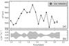 |
Fig. 1 Top: period spacing ΔP for the 19 dipole gravity modes observed in the Kepler SPB star KIC 10526294. Bottom: 1σ uncertainty region around each frequency |
The asymptotic period spacing for high-order low-degree gravity modes for a non-rotating star is given by 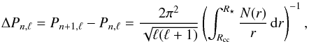 (2)where R⋆ is the stellar radius, Rcc indicates the boundary of the convective core, and Pn,ℓ and Pn + 1,ℓ are periods of two consecutive modes in radial order of the same degree ℓ (Tassoul 1980). In practice, the spatial integration is only carried out in the region where the g-modes propagate. Since we only consider consecutive dipole modes, we drop the n and ℓ subscripts from ΔPn,ℓ in the rest of the paper.
Figure 1a presents the sequence of 18 period spacings for the 19 consecutive dipole g-modes detected in KIC 10526294. They exhibit a small but clear deviation from the asymptotic (i.e. constant) period spacing relation in Eq. (2) and highlight the presence of chemical inhomogeneities that are left behind by the shrinking convective core (Miglio et al. 2008). In Fig. 1b, the frequency uncertainties σi of each frequency  are presented as a function of the mode periods.
During the MS phase, the core gradually shrinks and its density and pressure increase. Thus, the integrand in the right-hand side of Eq. (2) increases, and the asymptotic value ΔP as well as the structure of the period spacing sequence evolve. The former depends on the size of the fully mixed core, while the latter depends on the detailed treatment of mixing in the radiative envelope on top of the shrinking core (Miglio et al. 2008). Figure 2 shows the evolution of the asymptotic ΔP value computed from the right-hand side of Eq. (2) for three models with masses of 2.5 M⊙, 3.2 M⊙, and 3.8 M⊙. The observed period spacing range for KIC 10526294 from Table 1 is highlighted in grey. In practice, we chose the median frequency, f, from Table 1 and carried out the integration in the region where  (with Sℓ the Lamb frequency). Because the frequency range of f1 to f19 is limited, the choice of f does not alter the result of the integration, as we have verified. The asymptotic period spacing for models without overshooting (fov = 0.00, solid black lines) are mostly below those for models with overshooting (fov = 0.03, blue dashed lines). Varying the initial metallicity Zini introduces similar changes, which are not shown here for clarity.
Because several combinations of the stellar parameters can reproduce the same asymptotic ΔP value, it is essential to fit individual frequencies in addition to matching the asymptotic ΔP when performing seismic modelling. Based only on Fig. 2, both models at the low and high side of the mass range [ 3,4 ] M⊙ are able to explain the observed ΔP for KIC 10526294. Additional tuning and model selection requires scanning dense asteroseismic model grids that have a sufficiently broad range in mass M, but are also sufficiently fine in terms of all the other input parameters Xini, Zini, Xc, log Dmix, and fov, to obtain a meaningful result, according to the precision of the identified frequencies.
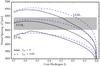 |
Fig. 2 Evolution of the asymptotic period spacing for dipole modes computed from the right-hand side of Eq. (2) versus Xc for models with masses 2.5 M⊙, 3.2 M⊙, and 3.8 M⊙, each for Zini = 0.020. The solid lines correspond to models without overshooting, while the dashed lines correspond to models including core overshooting with a value of fov = 0.03. The thin grey bar highlights the measured period range of 5048 to 5907 s for KIC 10526294 from Table 1; see also Fig. 1. All models were computed using OPAL opacity tables, and the Nieva & Przybilla (2012) and Przybilla et al. (2013) mixture. |
4. Extensive evolutionary and asteroseismic grids
P14 presented a dense evolutionary and asteroseismic grid of models dedicated to KIC 10526294; they considered relatively young models (Xc ≥ 0.40) in the range of 3.00 to 3.40 M⊙. Here, we followed the same approach, but we also included extra diffusive mixing beyond the convective and overshooting zones. Moreover, we varied several input parameters to study if that improves the quality of the frequency fitting compared to the one achieved by P14. We present eight evolutionary and asteroseismic grids in which some parameters are varied and some are kept fixed to keep the CPU requirements manageable.
The physical ingredients of the grids are the following. We used the open-source MESA1 code (Paxton et al. 2011, 2013) to calculate evolutionary tracks and store equilibrium models along each track for every 0.001 drop in Xc. This tiny grid step in the central hydrogen fraction was taken to ensure a small enough change in the frequency values of the modes as we follow the stellar evolution along an evolutionary track, relying on the numerical accuracy achieved by the MESA code coupled to the pulsation code we used (as discussed below), cf. Fig. 13 in P14 and its discussion.
We adopted the Ledoux convection criterion with a high semi-convective mixing coefficient given by αsc = 10-2 in the prescription by Langer et al. (1983). For this value, the Ledoux criterion is equivalent to the Schwarzschild criterion and ensures that ∇rad = ∇ad on the convective side of the core, following Gabriel et al. (2014). The mixing length parameter was set to αMLT = 1.8, while we fixed the initial composition to the Galactic standard given by Nieva & Przybilla (2012) and Przybilla et al. (2013, hereafter NP12): (Xini,Yini,Zini) = (0.710,0.276,0.014). We used the OPAL Type 1 (Rogers & Nayfonov 2002) opacity tables adapted to this mixture; these tables and the MESA inlists are available for download at the CDS (see Appendix C).
We adopted an exponentially decaying prescription for overshooting on top of the convective core in a diffusive approximation, following Freytag et al. (1996) and Herwig (2000): 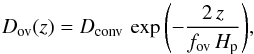 (3)where Dconv is the convective mixing coefficient, z = r − Rcc is the distance above the boundary of the convective core Rcc into the radiative region, and Hp is the local pressure scale height. The parameter fov governs the width of the overshooting layer, which in the framework of the mixing length theory of Böhm-Vitense (1958), is not constrained from first principles. We therefore treated it here as a free parameter and varied it in a broad range from 0.0 to 0.03 in all our grids.
 |
Fig. 3 Comparison between observed periods (vertical lines) and those of six models with different mixtures and opacity tables. All parameters of the models are identical, except their mixture and opacities. The widths of the vertical lines are larger than the measured pulsation period uncertainties. |
An alternative for core overshooting is to use a step-function prescription, which is commonly used in the literature. In this prescription, the overshooting extends over a distance dov = αovHp, beyond the convective core boundary. The material is treated as fully mixed in the overshoot range:  (4)where Rcc is the radial position of the boundary of the convective core, dov is the width of the overshooting zone and Dconv is the diffusion coefficient in the fully mixed convective core. Following the MESA implementation of core overshooting according to a step function, we tested explicitly that our seismic models are insensitive to the depth in the convective core at which the value of Dconv is picked up.
Our eight extensive evolutionary and asteroseismic grids are composed and named as follows:
-
Basic Grid: we investigated whether more massive and more evolved models may reproduce the observed, nearly flat, period spacing pattern of KIC 10526294 as well. The Basic Grid is essentially the extension of the grid in P14 towards higher masses and lower Xc.
-
Composition Grid: we calculated a grid varying Xini and Zini for the NP12 mixture to investigate if this improves the frequency fit.
-
Mixing Grid: various extra mixing mechanisms can operate and lead to smoothing of the composition profile outside the core. Unfortunately, we have no solid quantitative measures of the amount of extra mixing for B stars. Hence we computed a grid with models including extra diffusive mixing throughout the star for a wide range of log Dmix values.
-
Evolved Grid: a large amount of extra mixing combined with a low Xc may provide a situation for which the ΔP profile matches the observations for higher mass models. In Fig. 2, higher mass models cross the grey band at lower Xc. To ensure our age constraint is reliable, we calculated a grid for M ≥ 3.30 M⊙ incorporating extra mixing; we only considered the models whose mean ΔP falls inside the observed range in Fig. 2. Thus, the starting and ending Xc values for each track are flexible. This is the meaning of “–” in Table 2.
-
Fine Grid: to resolve the parameter space of mass, overshooting, and extra mixing, we increased the resolution for these parameters around the best model found from the Mixing Grid. Thus, we varied M ∈ [ 3.18, 3.27 ]M⊙ in steps of 0.01 M⊙, fov ∈ [ 0.016,0.019 ] in steps of 0.001, and log Dmix ∈ [ 0.25, 2.75 ] in steps of 0.25 dex.
-
Metallicity Grid: although the average metallicity of Galactic B stars in the solar neighbourhood is found to be Z = 0.014 ± 0.002 (Nieva & Przybilla 2012), individual B stars may still show a strong deviation from this average. Enhanced metallicity increases the height of the iron opacity bump and ensures better mode excitation. Moreover, as we demonstrate below in Fig. 5, the initial metallicity and mass exhibit a strong anti-correlation. To explore the possibility of our target having much higher metal abundance than the cosmic standard, we computed a grid identical to the Mixing Grid and Fine Grid, but with lower initial mass and higher initial metallicity up to Zini = 0.030.
-
Mixture Grids: the theoretical pulsation frequencies depend on the initial metal mixture and the adopted opacity tables. To illustrate this, Fig. 3 compares the observed periods (vertical grey lines) with those of six models with identical model parameters, except that they have different mixtures and opacities. The adopted mixtures for the grid are NP12, the solar mixture reported by Asplund et al. (2009; hereafter A09) and the Asplund et al. (2005) mixture with a Ne enhancement based on Cunha et al. (2006; hereafter A05+Ne). Figure 3 shows a clear difference in the frequency predictions, particularly for the longer-period modes. The relative difference in periods ranges from 0.07% to 0.14% from left to right in the figure. Changing the mixture in the models influences fitting high-precision frequencies of well-identified pulsation modes. In this respect, the asteroseismic data of KIC 10526294 bring us to the level where the dependence of the models on the assumed mixture can be tested for SPB stars, thanks to the identification of its dipole mode triplets. We calculated grids using both OP (Seaton 1987) and OPAL (Rogers & Nayfonov 2002) opacity tables for each of the NP12, A09, and A05+Ne mixtures. The parameter range for each of these sub-grids is identical. Once we found the best model in each sub-grid, we repeated the computations within a smaller range around the best model until the step size in mass, overshooting, metallicity, and log Dmix was 0.01, 0.001, 0.001 and 0.25 dex, respectively.
-
Step Function Overshoot Grid: to examine which of the two prescriptions for the core overshooting, exponentially decaying as in Eq. (3) versus step function as in Eq. (4), provides a better fit to the observed data, a stand-alone grid of models for a step function overshoot was computed around the best model from the Fine Grid, with the only change of using the step function instead of the exponential prescription for a range of masses and metallicities.
Table 2 gives the full parameter range in each of these grids. In the Mixing Grid and High Mass Grid, we varied the minimum diffusive mixing coefficient Dmix. For the Basic Grid and Composition Grid, we set Dmix = 0. In all grids except the Step Overshoot Grid, we used the exponential prescription as in Eq. (3). In total, our grids comprise 27 058 evolutionary tracks and around 4.3 million models that serve as input for the GYRE pulsation computations.
Eight model grids and their parameter range dedicated to the asteroseismic modelling of KIC 10526294.
For each input model, we used the state-of-the-art GYRE code (Townsend & Teitler 2013, version 3.0) to solve for the linear adiabatic oscillation frequencies of dipole ℓ = 1, m = 0 modes in the frequency range of the detected g-modes of KIC 10526294. The input inlist for the GYRE computations is available for download at the CDS; see Appendix C.
5. Model selection
5.1. Methodology
We considered a reduced  minimisation scheme to select the best-fitting models after comparing the observed frequencies
  with their model counterparts
  :
: 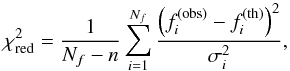 (5)where Nf = 19 is the number of consecutive g-modes and σi are the theoretical frequency uncertainties listed in Table 1. The number of degrees of freedom, n in Eq. (5), represents the number of independent model parameters. In all the cases, n is either 4 or 5, as listed in Table 2. This procedure is a simplified version of the goodness-of-fit adopted by P14, who also included the period spacing values in the χ2. Here, we prefered to forego this because demanding an optimal fit to the observed frequencies individually will automatically also deliver an optimal fit to the observed period spacing values. Moreover, we wished to compare the fit quality of models with a different number of degrees of freedom (n = 4 or 5, cf. Table 2) for the best model selection and this is better justified statistically when using independent measurements in the computation of .
The values in Eq. (5) gauge how well the model frequencies match the observed ones, where a value of 1 would mean that the input physics of the models is correct up to the level of the frequency precision. We are very far from this situation in the case of stars of spectral type O, B, or A. Indeed, for such massive stars, we are in a different situation compared to solar-like stars with stochastically excited oscillations, for which scaling relations can be applied to the Kepler data (Chaplin et al. 2014) and where extrapolations from the solar model are meaningful. In these straightforward cases, one achieves seismic modelling with typical values of  for the best Kepler data of G- or F-type stars on the main sequence, is achieved with a grid-based approach like the one we adopt here (Metcalfe et al. 2014). For the best modelled subgiants with solar-like oscillations, -values between 100 to 2000 were obtained (e.g. Deheuvels et al. 2014).
Seismic modelling of massive stars with heat-driven modes has not been done so far using the level of precision of the measured frequencies, cf. the discussion in Sect. 1 concerning the use of the Rayleigh limit as rough estimate of the measured frequency precision. Theoretical frequency predictions from models have typically only been computed up to 0.001 d-1, and the models were selected by visual inspection of the frequency spectra (e.g. Pamyatnykh et al. 2004) or by a χ2-type goodness-of-fit function ignoring the measured frequency precisions (e.g. Briquet et al. 2007). This is appropriate as a procedure when only a handful of identified mode frequencies is available. In this way, stellar masses, radii, core overshooting values, and ages have been deduced (e.g. Aerts 2015, for an overview).
5.2. Candidate models
Table 3 lists the parameters of the best-fit models for each of the grids described in Table 2. The first and second columns assign a number to each model and specify their grid of origin, respectively. The next eight columns specify the adopted input parameters for the best models. The last two columns give the (Eq. (5)) and values, respectively. The latter column is given to provide a sensible comparison with the results obtained from our previous modelling as discussed in P14 (their Table 6, Col. 11), where the input physics was kept fixed.
Model 1 is essentially the replication of the best model found in P14 from the Basic Grid, as a verification of the consistency between our previous and current study. Model 2 is taken from the Composition Grid. Comparison between Model 1 and Model 2 shows that, for the specific case of KIC 10526294, changing the initial composition Xini and Yini deteriorates the frequency fittings. Thus, the Galactic standard composition of B stars by Nieva & Przybilla (2012) is the most appropriate one to take for this target. Model 3 is the best of its kind from the Evolved Grid, but its is significantly higher than that of Model 1. Therefore, we exclude the possibility that KIC 10526294 is an evolved star.
Model 4 is taken from the Mixing Grid and the Fine Grid. It has the lowest score and is the best seismic model for KIC 10526294. It outperforms all models without diffusive mixing and is roughly 11 times better in fit quality than Model 1. Thus, we conclude that the frequency fitting for KIC 10526294 requires extra diffusive mixing with a value of log Dmix = 1.75 cm2 s-1. This is a similar conclusion as was reached for HD 50230 (Degroote et al. 2010), only this time we were able to quantify Dmix much more precisely and we considered various options for the metal mixture and opacities, while Z = 0.02 was fixed for HD 50230 and the degrees of its modes were not identified observationally. We find a value for the diffusive mixing coefficient of KIC 10526294 that is two orders of magnitude lower than the one for HD 50230. The two major differences between these stars are their mass and their Xc, both being ultra-slow rotators. It would be worth revisiting the seismic modelling of HD 50230 now that we are aware that it is a member of a spectroscopic binary and that p-modes have been found in addition to g-modes (Degroote et al. 2012); these two facts were not taken into account in the modelling efforts made by Degroote et al. (2010).
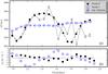 |
Fig. 4 a) Period and period spacings for Model 4 (filled circles) and Model 1 (empty squares) from Table 3. The observed pattern is shown in grey. b) The frequency difference between model frequencies and those detected in the observations δfi from Eq. (6). Compared to Fig. 1b, the ordinate is enlarged 40 times; the grey band around zero is the 1σ frequency uncertainty range σi. A similar plot for Model 4, Model 8, and Model 11 is shown in Figs. A.1 and A.2 in the Appendix. |
Models 5 to 9 originate from the Mixture sub-grids. They provide a test of the influence of different opacities and mixtures on the best values for Xc, fov and log Dmix. Regardless of their values, all these models converge to very similar values for Xc = 0.63 to 0.64, fov = 0.017 to 0.018, and log Dmix = 1.75 to 2.00. However, the mass varies somewhat and the metallicity varies widely over the scanned range. The fact that Xc, fov and log Dmix hardly depend on the mass, metallicity, mixture, and opacities manifests that a solid seismic constraint is placed on these values for the specific case of KIC 10526294. The discretisation of the grid parameters is also sufficiently optimal that the best values found are close to one another.
Models 5 and 8 have the A09 mixture and provide the fourth and third best fits to the frequencies, respectively. Although they are built from different opacities, the fit quality of these two models is indistinguishable in a statistical sense. Both are of lower fit quality than Model 4, given that the difference between their and the one of Model 4 is far above 3.84 (which would correspond to a p-value of 0.05 in the case of nested models). Furthermore, Model 4 and Model 7 have identical composition and mixture, but were calculated using OPAL and OP opacity tables, respectively. The parameters of these two models are very close in fit quality, although the latter has the worse . Models 6 and 9, with the A05+Ne mixture, also provide reasonably good fits to the frequencies. Therefore, changing the mixture, at least in this case, influences the adiabatic frequencies more than swapping between OP and OPAL opacity tables.
The of Model 10 is more than twice as high as the one of the best model. Hence, we come to the important conclusion that, for this slowly rotating SPB star the exponentially decaying prescription for core overshooting gives a better fit to the seismic data than a step function. A more reliable distinction between the two prescriptions for massive pulsators in general requires a reasonably large ensemble of B-type pulsators to be modelled with the two prescriptions. A re-analysis of the sample in Aerts (2015) could be highly instructive in this regard. Previously, Dziembowski & Pamyatnykh (2008) already considered an overshooting prescription based on two free parameters rather than a simple step function formulation in their modelling of the βCep stars νEri and 12 Lac, but these two pulsators did not allow firm conclusions on the shape of the overshooting.
Model 11 is selected from the Metallicity Grid, and is ranked as the second best asteroseismic model for our target. Even though it has a different initial mass and metallicity, the overshooting and extra mixing parameters perfectly agree with those of Model 4 to Model 9. Because Model 11 has 100% higher metal abundance than Model 4, it has a distinct stability property that is addressed in Sect. 6. Based on our minimisation, Model 4, and to a lesser extent Models 11 and 8, best represent the asteroseismic data of KIC 10526294. In the following sections, we use these three models for illustrative purposes.
5.3. Comparing best models and observations
Fig. 4a compares the observed period spacing (grey symbols) versus mode periods with those of Model 4 (filled circles) and Model 1 of P14 (empty squares), respectively. The resulting period spacing pattern of Model 4 clearly follows the observed pattern better than the pattern from Model 1 does. To appreciate how well the frequencies from Model 4 approach the observed ones, we show in Fig. 4b the frequency deviation δfi between the two through 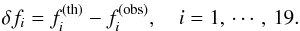 (6)In Fig. 4b, the ordinate range is 40 times larger than in Fig. 1b, and the 1σ frequency uncertainty band appears as a line here. The frequencies of Model 1 (empty squares) show stronger deviations from zero and the frequencies of Model 4 provide far better fits to the observed period series, especially in the lower period regime. To appreciate the quality of the model fit, we computed the average δfi for Model 4 and obtained 0.00051 d-1. While this is still a factor ~30 larger than the observational uncertainty on the frequencies, it is by far the best seismic model constructed to represent the pulsations of a late B-type star up to now.
Additional comparisons of the period spacing fits between Models 4 and 11 and between Models 8 and 11, are presented in Figs. A.1 and A.2 in the Appendix. We list the global parameters of the three best seismic models of KIC 10526294 in Table 4. Their structure variables (in GYRE-compatible format) are available at the CDS; see Appendix C. Even for optically bright B-type pulsators, the seismically derived effective temperature and surface gravity do not necessarily agree with their spectroscopic counterparts because the latter suffer from systematic uncertainties (e.g. Briquet et al. 2007, 2011). In the case of KIC 10526294, which is a faint star, the seismic values of the best models all agree with the spectroscopic values within 3σ, which we regard as good compatibility between seismology and spectroscopy.
Figure 5 shows the correlation diagrams between the five parameters of the Mixing Grid and the Fine Grid centred around the parameters of Model 4, that is, all panels present a subsurface in the space where the parameters that are not shown on the axes are fixed to the values found for Model 4. This is similar to Fig. 11 in P14, where semi-linear trends between all parameters occur. Here, we achieved more stringent constraints on some of the parameters, especially Xc, fov, and log Dmix (see also Fig. B.1). On the other hand, M and Z are less well constrained, although we achieved a relative precision below 4% for the mass. A strong linear correlation occurs between them, cf. panel (e), which is similar to Fig. 2 in Ausseloos et al. (2004). For a full overview of the distribution for the entire Mixing Grid, Fine Grid and Metallicity Grid, we refer to Fig. B.1 in the Appendix. The existence of correlations between the parameters hinders the derivation of appropriate uncertainties on the derived parameters of the best model(s), other than the bare minimum uncertainty given by the parameter stepsizes. A pragmatic estimate of the overall systematic and statistical uncertainty is provided by the ranges of the parameters of the best three models listed in Table 4.
Global parameters of Model 4, Model 8, and Model 11.
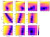 |
Fig. 5 Correlation diagram of the parameters of the Fine Grid around Model 4. Results are based on the Mixing Grid plus the Fine Grid. The colour coding is based on |
Based on Models 4, 8 and 11, we deduce that KIC 10526294 is a young star (Xc ≈ 0.63 to 0.64) of late-B spectral type. From the parameters of Models 4 to 9 and Model 11 in Table 3, the core overshoot parameter is tightly constrained in the range fov = 0.017 to 0.018. The overshooting zone has enough spatial and mass extension to allow partial trapping of some of the pulsation modes. This offers a unique opportunity for an in-depth study of the properties of the overshooting layer. Additionally, an extra diffusive mixing in the radiative part of the star of an amplitude log Dmix = 1.75 to 2.00 cm2 s-1 is needed to explain the observed frequencies. The parameters log Dmix, fov, and Xc only show a minor dependence on the adopted mixture and choice of the opacity tables.
One may question the success of our forward modelling for KIC 10526294, specifically given the high scores of the best model(s) in Table 3. We argue that despite such high values, the relative frequency deviations between the observed frequencies and those of the best seismic model remain below 0.4%. The left panels in Fig. 6 show  versus mode period
  for Model 4 (top) Model 8 (middle) and Model 11 (bottom), respectively. The strongest deviations occur for modes with periods exceeding ~1.68 days, that is, f1 to f8 in Table 1. For Model 4, the first eleven mode frequencies are very similar to the observed ones; the deviations gradually grow by increasing mode order. Current seismic models of solar-like stars observed with Kepler give rise to relative deviations of about 10-4 between observed and modelled frequencies near the frequency of maximum power (Metcalfe et al. 2014), but this is only achieved after applying an arbitrary surface correction (Kjeldsen et al. 2008). Our results are only an order of magnitude worse, but we are treating a star very different from the Sun; this is a major achievement. For completeness, we point out that we did not find any correlation between the mode amplitudes and the relative frequency deviations shown in Fig. 6.
The right panels in Fig. 6 show histograms of the relative frequency deviations between the measurements and theoretical predictions around zero. Despite the low-number statistics, the deviations for Model 4 are normally distributed, while those of the other two models do not show a clear Gaussian shape. For the solar-type pulsators, a frequency-dependent correction is applied to the theoretical frequencies to account for near-surface effects (e.g. Kjeldsen et al. 2008). For B-type pulsators, such a correction has so far been assumed to be unnecessary because these stars have a radiative envelope. If such surface a correction were needed for B-type stars, then we would have observed a monotonically deviating behaviour between the model frequencies and the observed ones, which is clearly not the case. Therefore, we argue that even if a surface correction term would be needed for KIC 10526294, it would be frequency-independent.
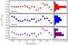 |
Fig. 6 Left panel: relative deviation between observed and modelled frequencies |
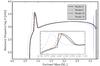 |
Fig. 7 Brunt-Väisälä frequency for Model 4 (black solid), Model 8 (red dashed), Model 10 (grey solid) and Model 11 (blue dotted) from Table 3 and Table 4. The inset is a zoom-in around the peak in the profile induced by the gradient of the mean molecular weight outside the convective core. These four models have different masses of the convective core Mcc. |
Figure 7 compares the profile of the Brunt-Väisälä frequency N(r), as used in Eq. (2) for four selected models. The inset is a zoom-in around the sharp increase in the profile, induced by the gradient of the mean molecular weight ∇μ outside the receding core. The profiles for Model 4 (black solid), Model 8 (red dashed) and Model 11 (blue dotted) are almost identical, because of their very similar overshooting parameter fov = 0.017 to 0.018, except for a slight shift in the position of the peak that is due to their different initial masses. The profile for Model 10 (grey solid) shows a steeper rise around 0.85 M⊙ because of the difference between the exponentially decaying and step function prescriptions for overshooting. The seismic frequency fitting indicates that the smoother shape of N(r) connected with the exponentially decaying prescription is to be preferred over the steep step-function for KIC 10526294.
6. Mode excitation
In their Fig. 14, P14 already showed a mismatch between the predicted and observed excited modes using their best model (i.e. Model 1 here). Only eleven modes out of nineteen in Model 1 are excited. Aside from the forward modelling, we examined if our improved modelling remedies that shortcoming. For this, we used the non-adiabatic framework of GYRE (version 3.2.2).
It is well known that current predictions of mode excitation through the heat mechanism are not yet sufficiently appropriate to explain all the detected and identified modes in B-type stars (Dziembowski & Pamyatnykh 2008). For this reason, we examined the mode stability properties of our best models a posteriori.
Miglio et al. (2007) already suggested that adopting OP opacity tables instead of OPAL might remedy the mode excitation problem. As a result of the significant role of the opacity profile in mode excitation, we first considered its profile in three of the best selected models. Figure 8 compares the Rosseland mean opacity profile κ versus temperature log T in Model 4 (black solid line, using OPAL), Model 8 (red dashed line, using OP) and Model 11 (blue dashed-dotted line, using OPAL). The inset is a zoom in of the Fe opacity bump. Obviously, Model 11, with its twice as high initial metallicity Zini is more opaque than the other two. Moreover, Model 8 is more opaque than Model 4 despite their nearly identical Zini, because the former model uses the OP opacities, in line with Miglio et al. (2007).
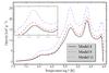 |
Fig. 8 Rosseland mean opacity profile in Model 4 (Zini = 0.014, OPAL, NP12, black solid line), Model 8 (Zini = 0.015, OP, A09, red dashed-dotted line) and Model 11 (Zini = 0.028, OPAL, NP12, blue dashed line) versus temperature. The inset is a zoom around the iron-bump of opacity. The iron opacity peak for the OP model occurs at slightly hotter interior. |
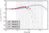 |
Fig. 9 Non-adiabatic instability study of Model 4 (black circles), Model 8 (red squares), and Model 11 (blue stars) from Table 3. The imaginary part of the eigenfrequency ωIm is plotted against the mode period (vertical lines). Filled (empty) symbols designate excited (damped) modes. |
In Fig. 9, we compare the growth rate (i.e. the imaginary part of the complex eigenfrequency ωIm) as a function of mode period for Model 4 (black circles), Model 8 (red squares) and Model 11 (blue stars), respectively. The vertical lines are the observed periods. The excited (damped) modes are shown with filled (empty) symbols. Although Model 4 reproduces the real part of eigenfrequencies better than Model 11, the latter predicts more excited modes than observed. This is not a surprise given the high Zini of Model 11, which implies a ~70% higher iron opacity (see Fig. 8). We point out that an ad-hoc local increase in the height of the iron opacity bump by up to ~50% (cf. Pamyatnykh et al. 2004) would allow Model 4 (as well as other models from the Mixing Grid and Fine Grid) to have equally good mode excitation properties as Model 11. Model 8 has two additional excited modes compared to those of Model 4, despite both having similar Zini. This is as expected because OP opacities predict more excited modes (Miglio et al. 2007). Additionally, all three models presented here predict two to four short-period modes to be excited but these are not among the detected modes listed in P14.
The distinction between Model 4, Model 8 and Model 11 is not clear-cut; the former offers the best adiabatic frequency match with the observations, while the latter explains the mode excitation better at the cost of a somewhat poorer frequency fitting. Additionally, the metallicity value Zini of Model 4 and of Model 8 perfectly agrees with the Galactic standard composition of Nieva & Przybilla (2012) for nearby B stars, while Model 11 is twice as metal-rich as the standard. Given the current lack of a higher signal-to-noise spectrum in addition to the one presented in P14 upon which we relied, we cannot evaluate this metallicity difference between the best models from spectroscopic abundance analysis. Fortunately, this degeneracy does not affect the seismic estimates of the core overshooting and diffusive mixing deduced for the star.
7. Discussion and conclusions
Forward seismic modelling based on the 19 detected and identified dipole gravity modes of the B8.3V star KIC 10526294 led to the derivation of its mass, radius, and age within the ranges M ∈ [ 3.13,3.25 ] M⊙, R ∈ [ 2.19,2.38 ] R⊙, and age [ 62,92 ] Myr, respectively. These ranges cannot be refined to tighter constraints as long as we do not have a constrained metallicity from spectroscopy. In practice, the range of Z ∈ [ 0.014,0.028 ] leads to good seismic models in this mass range, and the (M,Z) correlation implies a quite large uncertainty on the seismic age. However, the seismic data do require the inclusion of a small but significant amount of extra diffusive mixing in the radiative envelope of the star, with a value of log Dmix in the range [ 1.75,2.00 ] cm2 s-1, in addition to an exponentially decaying core overshooting with parameter fov ∈ [ 0.017,0.018 ]. The tight constraints on log Dmix and fov do not depend on the choice of the mass, metallicity, mixture and opacity table within the allowed seismic ranges. We also conclude that models with a step function core overshooting description are of inferior quality to explain the seismic data of this star.
Our work represents the first application of seismic modelling of an SPB from which the need of global extra mixing is proven and quantified with high precision, based on the observed frequencies of unambiguously identified modes. Addressing the origin of the physical mechanisms that generate the desired value of Dmix, and their possible interaction(s), is yet to be done, keeping in mind that KIC 10526294 is an ultra-slow rotator.
Forward seismic modelling is currently the best starting point to describe the global physical parameters, the interior structure characteristics, and the detailed pulsational properties of real stars. To carry out an iterative asteroseismic inversion for the rotation profile or for the entire structure of the star, one has to start from a calibrated model that has the ability to fit all the detected and identified oscillation modes reasonably close to their measured frequencies. In this study, we have achieved this for the slowly rotating Kepler target KIC 10526294.
Despite the still relatively high  values for the best model(s), Fig. 6 shows that the relative deviation between the modelled and observed frequencies is below 0.4%. Incorporating non-adiabatic corrections to the adiabatic frequencies, and moving beyond the linearised oscillation paradigm (e.g. Van Hoolst 1994) may further reduce the deviations between the observed and model frequencies. In addition, there is still room for improving the mode stability predictions for KIC 10526294 because (a) depending on the adopted metallicity, several of the observed longest-period dipole modes are predicted to be stable, and (b) few excited dipole modes are not observed.
Thanks to the unprecedented precision of the observations assembled by the nominal Kepler mission, we have now reached the stage at which we can employ asteroseismic methods to calibrate the internal structure of massive stars with well-developed convective cores, and quantify the level of seismic modelling. This allows us to evaluate different choices of the input physics of B-star models coupled with an appropriate statistical framework (such as the ) to properly account for the difference of the models. Our modelling of KIC 10526294 proves that we can adequately explain the high-precision data collected from space within the framework of spherically symmetric stellar evolution models, and a linearised formalism of stellar oscillations below percent level.
Online material
Appendix A: Period spacing for iternative models
The comparison between the period spacing of the first and second best models is presented in Fig. A.1. A similar plot for the second and third best models is shown in Fig. A.2. Both Model 8 and Model 11 provide poorer fits to the period spacing on the short-period range of the series, than Model 4 (Fig. 4).
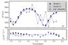 |
Fig. A.1 Top panel: period spacing for Model 4 (filled circles) and Model 11 (empty squares). See Table 3 for their parameters. Bottom panel: absolute frequency deviations of the two models with respect to observations. See also Fig. 4 for a comparison. |
Appendix B: Full overview of the Mixing, Fine and Metallicity grids
The Mixing, Fine and Metallicity grids introduced in Table 2 have identical physical ingredients, and it is safe to merge their goodness-of-fit into a single snapshot. Figure B.1 shows  as a function of the dimensions of the three grids in addition to the model radius and surface gravity. Note the finger-like structures in panels (c), (g), and (h) where the age, overshooting and mixing parameters are constrained, respectively. In panel (i), the position of all models is shown on the Kiel diagram (log Teff vs. log g), and that of the best model is marked with a (white) star. Our Model 4 is found marginally inside the 2σ uncertainty box from spectroscopy.
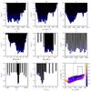 |
Fig. B.1 Behaviour of |

Appendix C: Deliverables, inlists, and opacity tables
We adhere to the MESA code of conduct as stated in Paxton et al. (2011), and make our setting files and physical ingredients publicly available for download. This also ensures reproducibility of our results. The following items are available at the CDS:
-
The MESA v.5548 input inlists,
-
The GYRE v.3.0 inlist,
-
The OP and OPAL opacity tables adapted to the A05+Ne, A09, and NP12 mixtures. They have to be used with a standard MESA composition optioninitial_zfracs = 5, 6 and 8, respectively. All tables are MESA compatible. When querying the OP and OPAL servers, we made a choice to redistribute the abundance residuals on all metals, based on their relative mass fraction instead of depositing them on the heaviest metals, which are Fe and Ni. This is a choice and may slightly influence the adiabatic and non-adiabatic results.
-
The internal structure of Model 4, Model 5, Model 8, Model 10, and Model 11 in a GYRE-compatible format.
Static links to download each of these products are available at https://fys.kuleuven.be/ster/Projects/ASAMBA at the CDS.
MESA can be downloaded from the project Web site http://mesa.sourceforge.net
Acknowledgments
We are grateful to the valuable comments from the anonymous referee. E.M. is beneficiary of a postdoctoral grant from the Belgian Federal Science Policy Office, co-funded by the Marie Curie Actions FP7-PEOPLE-COFUND-2008 n°246540 MOBEL GRANT from the European Commission. Part of the research included in this manuscript was based on funding from the Research Council of KU Leuven under grant GOA/2013/012 and from the National Science Foundation of the USA under grant No. NSF PHY11-25915. The computational resources and services used in this work were provided by the VSC (Flemish Supercomputer Center), funded by the Hercules Foundation and the Flemish Government department EWI. E.M. and C.A. thank Bill Paxton, Richard Townsend, and Francis Timmes for their valuable support with the MESA and GYRE codes, Steven Kawaler for fruitful discussions about period spacings, and Andrea Miglio for various discussions on extra diffusive mixing over the past years. C.A. and P.I.P. acknowledge the staff of the Kavli Institute of Theoretical Physics at the University of California, Santa Barbara, for the kind hospitality during the 2015 research programme “Galactic Archaeology and Precision Stellar Astrophysics”. E.M. is grateful to the organisers of IAU 307 symposium in Geneva where part of this work was presented.
References
- Aerts, C. 2015, IAU Symp., 307, 164 [Google Scholar]
- Aerts, C., Molenberghs, G., Kenward, M. G., & Neiner, C. 2014, ApJ, 781, 88 [NASA ADS] [CrossRef] [Google Scholar]
- Asplund, M., Grevesse, N., & Sauval, A. J. 2005, in Cosmic Abundances as Records of Stellar Evolution and Nucleosynthesis, eds. T. G. Barnes III, & F. N. Bash, ASP Conf. Ser., 336, 25 [Google Scholar]
- Asplund, M., Grevesse, N., Sauval, A. J., & Scott, P. 2009, ARA&A, 47, 481 [NASA ADS] [CrossRef] [Google Scholar]
- Ausseloos, M., Scuflaire, R., Thoul, A., & Aerts, C. 2004, MNRAS, 355, 352 [NASA ADS] [CrossRef] [Google Scholar]
- Böhm-Vitense, E. 1958, Z. Astrophys., 46, 108 [Google Scholar]
- Briquet, M., Morel, T., Thoul, A., et al. 2007, MNRAS, 381, 1482 [NASA ADS] [CrossRef] [Google Scholar]
- Briquet, M., Aerts, C., Baglin, A., et al. 2011, A&A, 527, A112 [NASA ADS] [CrossRef] [EDP Sciences] [Google Scholar]
- Chaboyer, B. 1994, PASP, 106, 200 [NASA ADS] [CrossRef] [Google Scholar]
- Chaplin, W. J., Basu, S., Huber, D., et al. 2014, ApJS, 210, 1 [NASA ADS] [CrossRef] [Google Scholar]
- Charbonnel, C., Vauclair, S., & Zahn, J.-P. 1992, A&A, 255, 191 [NASA ADS] [Google Scholar]
- Cunha, K., Hubeny, I., & Lanz, T. 2006, ApJ, 647, L143 [NASA ADS] [CrossRef] [Google Scholar]
- De Cat, P., & Aerts, C. 2002, A&A, 393, 965 [NASA ADS] [CrossRef] [EDP Sciences] [Google Scholar]
- Degroote, P., Briquet, M., Catala, C., et al. 2009, A&A, 506, 111 [NASA ADS] [CrossRef] [EDP Sciences] [Google Scholar]
- Degroote, P., Aerts, C., Baglin, A., et al. 2010, Nature, 464, 259 [NASA ADS] [CrossRef] [PubMed] [Google Scholar]
- Degroote, P., Aerts, C., Michel, E., et al. 2012, A&A, 542, A88 [NASA ADS] [CrossRef] [EDP Sciences] [Google Scholar]
- Deheuvels, S., Doğan, G., Goupil, M. J., et al. 2014, A&A, 564, A27 [NASA ADS] [CrossRef] [EDP Sciences] [Google Scholar]
- Ding, C. Y., & Li, Y. 2014, MNRAS, 438, 1137 [NASA ADS] [CrossRef] [Google Scholar]
- Dziembowski, W. A., & Pamyatnykh, A. A. 1991, A&A, 248, L11 [NASA ADS] [Google Scholar]
- Dziembowski, W. A., & Pamyatnykh, A. A. 2008, MNRAS, 385, 2061 [NASA ADS] [CrossRef] [Google Scholar]
- Freytag, B., Ludwig, H.-G., & Steffen, M. 1996, A&A, 313, 497 [Google Scholar]
- Gabriel, M., Noels, A., Montalban, J., & Miglio, A. 2014, A&A, 569, A63 [NASA ADS] [CrossRef] [EDP Sciences] [Google Scholar]
- Heger, A., Langer, N., & Woosley, S. E. 2000, ApJ, 528, 368 [NASA ADS] [CrossRef] [Google Scholar]
- Heger, A., Woosley, S. E., & Spruit, H. C. 2005, ApJ, 626, 350 [NASA ADS] [CrossRef] [Google Scholar]
- Herwig, F. 2000, A&A, 360, 952 [NASA ADS] [Google Scholar]
- Huang, W., Gies, D. R., & McSwain, M. V. 2010, ApJ, 722, 605 [NASA ADS] [CrossRef] [Google Scholar]
- Jeans, J. H. 1928, Astronomy and cosmogony (Cambridge University Press) [Google Scholar]
- Kato, S. 1966, PASJ, 18, 374 [NASA ADS] [Google Scholar]
- Kjeldsen, H., Bedding, T. R., & Christensen-Dalsgaard, J. 2008, ApJ, 683, L175 [NASA ADS] [CrossRef] [Google Scholar]
- Langer, N., Fricke, K. J., & Sugimoto, D. 1983, A&A, 126, 207 [NASA ADS] [Google Scholar]
- Maeder, A. 2009, Physics, Formation and Evolution of Rotating Stars, ed. A. Maeder (Berlin, Heidelberg: Springer) [Google Scholar]
- Maeder, A., Meynet, G., Lagarde, N., & Charbonnel, C. 2013, A&A, 553, A1 [NASA ADS] [CrossRef] [EDP Sciences] [Google Scholar]
- Metcalfe, T. S., Creevey, O. L., Doğan, G., et al. 2014, ApJS, 214, 27 [NASA ADS] [CrossRef] [Google Scholar]
- Miglio, A., Montalbán, J., & Dupret, M.-A. 2007, MNRAS, 375, L21 [CrossRef] [Google Scholar]
- Miglio, A., Montalbán, J., Noels, A., & Eggenberger, P. 2008, MNRAS, 386, 1487 [NASA ADS] [CrossRef] [Google Scholar]
- Nieva, M.-F., & Przybilla, N. 2012, A&A, 539, A143 [NASA ADS] [CrossRef] [EDP Sciences] [Google Scholar]
- Pamyatnykh, A. A., Handler, G., & Dziembowski, W. A. 2004, MNRAS, 350, 1022 [NASA ADS] [CrossRef] [Google Scholar]
- Pápics, P. I., Moravveji, E., Aerts, C., et al. 2014, A&A, 570, A8 [NASA ADS] [CrossRef] [EDP Sciences] [Google Scholar]
- Paxton, B., Bildsten, L., Dotter, A., et al. 2011, ApJS, 192, 3 [Google Scholar]
- Paxton, B., Cantiello, M., Arras, P., et al. 2013, ApJS, 208, 4 [NASA ADS] [CrossRef] [Google Scholar]
- Przybilla, N., Nieva, M. F., Irrgang, A., & Butler, K. 2013, in EAS PS, 63, 23 [Google Scholar]
- Rogers, F. J., & Nayfonov, A. 2002, ApJ, 576, 1064 [Google Scholar]
- Roxburgh, I. W. 1965, MNRAS, 130, 223 [NASA ADS] [Google Scholar]
- Saslaw, W. C., & Schwarzschild, M. 1965, ApJ, 142, 1468 [NASA ADS] [CrossRef] [Google Scholar]
- Schwarzenberg-Czerny, A. 1991, MNRAS, 253, 198 [NASA ADS] [CrossRef] [Google Scholar]
- Schwarzschild, M., & Härm, R. 1958, ApJ, 128, 348 [NASA ADS] [CrossRef] [Google Scholar]
- Seaton, M. J. 1987, J. Phys. B Atomic Molecular Physics, 20, 6363 [Google Scholar]
- Shaviv, G., & Salpeter, E. E. 1973, ApJ, 184, 191 [NASA ADS] [CrossRef] [Google Scholar]
- Szewczuk, W., Daszyńska-Daszkiewicz, J., & Dziembowski, W. 2014, in IAU Symp. 301, eds. J. A. Guzik, W. J. Chaplin, G. Handler, & A. Pigulski, 109 [Google Scholar]
- Tassoul, M. 1980, ApJS, 43, 469 [NASA ADS] [CrossRef] [Google Scholar]
- Townsend, R. H. D., & Teitler, S. A. 2013, MNRAS, 435, 3406 [NASA ADS] [CrossRef] [Google Scholar]
- Van Hoolst, T. 1994, A&A, 286, 879 [NASA ADS] [Google Scholar]
- Waelkens, C. 1991, A&A, 246, 453 [NASA ADS] [Google Scholar]
- Weiss, A., Hillebrandt, W., & Truran, J. W. 1988, A&A, 197, L11 [NASA ADS] [Google Scholar]
- Zahn, J.-P. 1992, A&A, 265, 115 [NASA ADS] [Google Scholar]
All Tables
Frequencies , periods , period spacings , and 1σ errors of the central peaks (m = 0) of the dipole (ℓ = 1) triplets observed in KIC 10526294 as determined from Table B.1 in P14.
Eight model grids and their parameter range dedicated to the asteroseismic modelling of KIC 10526294.
All Figures
|
Fig. 1 Top: period spacing ΔP for the 19 dipole gravity modes observed in the Kepler SPB star KIC 10526294. Bottom: 1σ uncertainty region around each frequency |
| In the text | |
|
Fig. 2 Evolution of the asymptotic period spacing for dipole modes computed from the right-hand side of Eq. (2) versus Xc for models with masses 2.5 M⊙, 3.2 M⊙, and 3.8 M⊙, each for Zini = 0.020. The solid lines correspond to models without overshooting, while the dashed lines correspond to models including core overshooting with a value of fov = 0.03. The thin grey bar highlights the measured period range of 5048 to 5907 s for KIC 10526294 from Table 1; see also Fig. 1. All models were computed using OPAL opacity tables, and the Nieva & Przybilla (2012) and Przybilla et al. (2013) mixture. |
| In the text | |
|
Fig. 3 Comparison between observed periods (vertical lines) and those of six models with different mixtures and opacity tables. All parameters of the models are identical, except their mixture and opacities. The widths of the vertical lines are larger than the measured pulsation period uncertainties. |
| In the text | |
|
Fig. 4 a) Period and period spacings for Model 4 (filled circles) and Model 1 (empty squares) from Table 3. The observed pattern is shown in grey. b) The frequency difference between model frequencies and those detected in the observations δfi from Eq. (6). Compared to Fig. 1b, the ordinate is enlarged 40 times; the grey band around zero is the 1σ frequency uncertainty range σi. A similar plot for Model 4, Model 8, and Model 11 is shown in Figs. A.1 and A.2 in the Appendix. |
| In the text | |
|
Fig. 5 Correlation diagram of the parameters of the Fine Grid around Model 4. Results are based on the Mixing Grid plus the Fine Grid. The colour coding is based on |
| In the text | |
|
Fig. 6 Left panel: relative deviation between observed and modelled frequencies |
| In the text | |
|
Fig. 7 Brunt-Väisälä frequency for Model 4 (black solid), Model 8 (red dashed), Model 10 (grey solid) and Model 11 (blue dotted) from Table 3 and Table 4. The inset is a zoom-in around the peak in the profile induced by the gradient of the mean molecular weight outside the convective core. These four models have different masses of the convective core Mcc. |
| In the text | |
|
Fig. 8 Rosseland mean opacity profile in Model 4 (Zini = 0.014, OPAL, NP12, black solid line), Model 8 (Zini = 0.015, OP, A09, red dashed-dotted line) and Model 11 (Zini = 0.028, OPAL, NP12, blue dashed line) versus temperature. The inset is a zoom around the iron-bump of opacity. The iron opacity peak for the OP model occurs at slightly hotter interior. |
| In the text | |
|
Fig. 9 Non-adiabatic instability study of Model 4 (black circles), Model 8 (red squares), and Model 11 (blue stars) from Table 3. The imaginary part of the eigenfrequency ωIm is plotted against the mode period (vertical lines). Filled (empty) symbols designate excited (damped) modes. |
| In the text | |
|
Fig. A.1 Top panel: period spacing for Model 4 (filled circles) and Model 11 (empty squares). See Table 3 for their parameters. Bottom panel: absolute frequency deviations of the two models with respect to observations. See also Fig. 4 for a comparison. |
| In the text | |
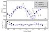 |
Fig. A.2 Similar to Fig. 4 but for Model 8 (filled circles) and Model 11 (empty squares). |
| In the text | |
|
Fig. B.1 Behaviour of |
| In the text | |
Current usage metrics show cumulative count of Article Views (full-text article views including HTML views, PDF and ePub downloads, according to the available data) and Abstracts Views on Vision4Press platform.
Data correspond to usage on the plateform after 2015. The current usage metrics is available 48-96 hours after online publication and is updated daily on week days.
Initial download of the metrics may take a while.