| Issue |
A&A
Volume 579, July 2015
|
|
|---|---|---|
| Article Number | A108 | |
| Number of page(s) | 12 | |
| Section | Stellar structure and evolution | |
| DOI | https://doi.org/10.1051/0004-6361/201526123 | |
| Published online | 09 July 2015 | |
The little-studied cluster Berkeley 90
I. LS III +46 11: a very massive O3.5 If* + O3.5 If* binary
1 Centro de Astrobiología, CSIC-INTA, campus ESAC, apartado postal 78, 28 691 Villanueva de la Cañada, Madrid, Spain
e-mail: This email address is being protected from spambots. You need JavaScript enabled to view it.
2 Departamento de Física, Ingeniería de Sistemas y Teoría de la Señal, Escuela Politécnica Superior, Universidad de Alicante, PO Box 99, 03 080 Alicante, Spain
3 Departamento de Física y Astronomía, Universidad de La Serena, Av. Cisternas 1200 Norte, La Serena, Chile
4 Space Telescope Science Institute, 3700 San Martin Drive, Baltimore, MD 21 218, USA
5 Department of Physics & Astronomy, 1 College Circle, SUNY Geneseo, Geneseo, NY 14 454, USA
6 Instituto de Astrofísica de Canarias, 38 200 La Laguna, Tenerife, Spain
7 Departamento de Astrofísica, Universidad de La Laguna, 38 205 La Laguna, Tenerife, Spain
8 Instituto de Astrofísica de Andalucía-CSIC, Glorieta de la Astronomía s/n, 18 008 Granada, Spain
9 Instituto de Astrofísica de La Plata (CCT La Plata-CONICET, Universidad Nacional de La Plata), Paseo del Bosque s/n, 1900 La Plata, Argentina
Received: 18 March 2015
Accepted: 25 April 2015
Abstract
Context. It appears that most (if not all) massive stars are born in multiple systems. At the same time, the most massive binaries are hard to find owing to their low numbers throughout the Galaxy and the implied large distances and extinctions.
Aims. We want to study LS III +46 11, identified in this paper as a very massive binary; another nearby massive system, LS III +46 12; and the surrounding stellar cluster, Berkeley 90.
Methods. Most of the data used in this paper are multi-epoch high S/N optical spectra, although we also use Lucky Imaging and archival photometry. The spectra are reduced with dedicated pipelines and processed with our own software, such as a spectroscopic-orbit code, CHORIZOS, and MGB.
Results. LS III +46 11 is identified as a new very early O-type spectroscopic binary [O3.5 If* + O3.5 If*] and LS III +46 12 as another early O-type system [O4.5 V((f))]. We measure a 97.2-day period for LS III +46 11 and derive minimum masses of 38.80 ± 0.83 M⊙ and 35.60 ± 0.77 M⊙ for its two stars. We measure the extinction to both stars, estimate the distance, search for optical companions, and study the surrounding cluster. In doing so, a variable extinction is found as well as discrepant results for the distance. We discuss possible explanations and suggest that LS III +46 12 may be a hidden binary system where the companion is currently undetected.
Key words: binaries: spectroscopic / dust, extinction / ISM: lines and bands / stars: early-type / stars: individual: LS III +46 11 / open clusters and associations: individual: Berkeley 90
© ESO, 2015
1. Introduction
Multiplicity is an endemic disease among O stars (Mason et al. 1998; Sana et al. 2013a; Sota et al. 2014). Indeed, it is difficult to find an O star that was born in isolation. Among the Sota et al. (2014) sample of O7-O9.7 V-IV stars south of −20 deg, there is just one clear, currently single object, namely μ Col; it is, however, a known runaway and thus was likely born in a multiple system or compact cluster. Only a small fraction of the other types of O stars in the Sota et al. (2014) sample are apparently single, but those cases are more luminous and can easily hide a main-sequence B-type companion, for example, in their glare. Both types of binarity, spectroscopic and visual, are common among O stars and combinations of both types (implying higher-order multiplicities) are also relatively frequent, usually in the form of hierarchical systems, with one pair in a close orbit and additional star(s) at larger separations. The OWN survey (Barbá et al. 2010) has detected a peak around 10 days in the spectroscopic period distribution of 240 southern massive stars. Most of those systems will interact during their evolution and many mergers are expected (Sana et al. 2012). Even in those cases where interactions will not take place it is important to characterize the binarity of O stars since ignoring it can lead to biases in the measured properties, such as derived masses and predicted colors of small stellar populations or young clusters.
The issue of multiplicity among massive stars also affects the measurement of the stellar upper mass limit since one has to make sure that a very luminous object is not in reality a combination of two or more objects, an issue that has produced a number of false alarms in the past (see, e.g., Maíz Apellániz et al. 2007). For a long time, it was thought that all very massive stars were born as very early O-type objects, but the most current information leans towards the extremely massive ones being born as WNh stars (Crowther et al. 2010). However, the very poor statistics means that the case cannot be considered closed. For example, only one O2 star with accurate blue-violet spectral classification is known in the Milky Way, HD 93 129 AaAb (Sota et al. 2014), and it is a multiple system located in the center of a dense stellar cluster. We clearly need to find more very massive stars to understand their properties and evolution.
The sparse young open cluster Berkeley 90 (Fig. 1) is almost unstudied, but Sanduleak (1974) suggested that the early-type stars LS III +46 11 and LS III +46 12 were members of the cluster. Both objects are classified as OB+ in the Luminous Stars catalogue (Hardorp et al. 1964), suggesting high luminosities. From an analysis of 2MASS data for the region, Tadross (2008) concluded that the cluster was young (<100 Ma old), located at 2.4 kpc, and reddened by E(B − V) = 1.15 mag. Wendker (1971) suggested that LS III +46 11 and LS III +46 12 were the ionizing sources for the H ii region [GS55] 215, which can be identified with Sh 2-115 (Harten & Felli 1980). Mayer & Macák (1973) derived a spectral type O6 and a distance of 2.3 kpc for LS III +46 12, but were unable to provide a spectral type for LS III +46 11, which is more reddened. LS III +46 11 was identified as the counterpart of the moderately hard ROSAT source RX J2035.2+4651 by Motch et al. (1997) during a search for possible high-mass X-ray binaries. They derived a spectral type O3-5 III(f)e from intermediate-resolution spectroscopy, and concluded that LS III +46 11 could produce the observed X-ray luminosity of ∼5 × 1033erg s-1 with “probably no need” for a compact companion but that “the extreme value of the X-ray luminosity of this star would certainly deserve further detailed investigation” without mentioning an alternative (e.g., a colliding-wind binary). Motch et al. (1997) also detected an X-ray source coincident with LS III +46 12 with about one third of the X-ray flux of LS III +46 11.
As part of our Galactic O-Star Spectroscopic Survey (GOSSS, Maíz Apellániz et al. 2011), we observed LS III +46 11 with the TWIN spectrograph of the 3.5 m telescope at Calar Alto in early November 2009. We immediately confirmed the very early nature of the system, but more surprising was the double-lined spectroscopic binary (SB2) nature detected in the He ii lines. Given the importance of the discovery, we observed the system on three consecutive nights (1, 2, and 3 November) and we noticed only a small decrease in the velocity separation, thus excluding a short period. For the next two years we reobserved LS III +46 11 on different occasions, but we failed to detect clearly split He ii lines until September 2011, when we observed it with the 4.2 m WHT at La Palma. The new detection gave us a series of possible periods for the system and led to new observations in the subsequent years. By 2013 we had a preliminary orbit with a period close to 97 days and by 2014 we obtained the final orbit, which had a large eccentricity that explained the measurement difficulties.
In this paper first we describe the data used, both the primary spectroscopic observations and the complementary high-resolution imaging and archival photometry. We then present our results: the spectral classification of LS III +46 11 and LS III +46 12, the spectroscopic orbit of LS III +46 11, the extinction and distance to both stars, a search for visual companions, and a global analysis of Berkeley 90. Finally, we discuss our results, including their relevance for the study of the stellar upper mass limit, and present our conclusions. In a subsequent paper we will analyze the foreground ISM in front of Berkeley 90.
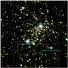 |
Fig. 1 2MASS KSHJ three-color RGB mosaic of Berkeley 90. The intensity level in each channel is logarithmic. |
LS III +46 11 and LS III +46 12 summary.
2. Data
2.1. Spectroscopy
Spectroscopic observation log for LS III +46 11. The date refers to the local evening.
Spectroscopic observation log for LS III +46 12. The date refers to the local evening.
The spectroscopic data for LS III +46 11 used in this paper were obtained with six different telescopes and are listed in Table 2. Here we describe the data grouped under the different projects in which they were obtained.
-
1.
GOSSS: the Galactic O-Star Spectroscopic Sur-vey is described in Maíz Apellánizet al. (2011). The GOSSSspectra used here were obtained with the TWIN spec-trograph of the 3.5 m tele-scope at Calar Alto (CAHA) and the ISIS spectrographof the 4.2 m William Herschel Telescope(WHT) at La Palma. The spectral resolving power wasmeasured in each case1 and were determined to be be-tween 2800 and 3400 (TWIN)and between 3900 and 5400(ISIS). The typical signal-to-noise ratio (S/N) per resolutionelement of the data is 300. The spectral range of the WHT dataincludes both He iiλ4541.591and He iiλ5411.53, while thatof the CAHA-3.5 m data included only the for-mer2. GOSSSalso obtained spectroscopy with the Albireo spectrograph ofthe 1.5 m telescope at the Observa-torio de Sierra Nevada (OSN), but its aperture is too small to obtaina good S/N in the blue-violet. However, we also obtained someOSN yellow-red spectra at R ∼ 2000 in order to study He iiλ5411.53.
-
2.
NoMaDS: the Northern Massive Dim Survey is described in Maíz Apellániz et al. (2012) and Pellerin et al. (2012). NoMaDs spectra were obtained with the High Resolution Spectrograph of the 9 m Hobby-Eberly Telescope (HET) at McDonald Observatory. Their spectral resolving power is 30 000 and all epochs include He iiλ5411.53 though two different setups were used on different occasions: one that goes from the violet to the yellow with a small gap (3811–4709 Å + 4758–5735 Å) and one that goes from the green to the red with another small gap (5311–6275 Å + 6396–7325 Å).
-
3.
IACOB: the Instituto de Astrofísica de Canarias OB database is described in Simón-Díaz et al. (2011) and Simón-Díaz et al. (2015b). IACOB spectra were obtained with the FIES spectrograph at the 2.6 m Nordic Optical Telescope (NOT) at la Palma. Their spectral resolving power is 23 000 and they cover the whole optical range. Some epochs were obtained as part of IACOB itself and some were obtained during service time after a request to observe LS III +46 11 was granted additional time.
-
4.
CAFÉ-BEANS: the Calar Alto Fiber-fed Échelle Binary Evolution Andalusian Northern Survey is described in Negueruela et al. (2015). CAFÉ-BEANS spectra were obtained with the CAFÉ spectrograph at the 2.2 m telescope at Calar Alto. Their spectral resolving power is 65 000 and they cover the whole optical range.
The spectroscopic data for LS III +46 12 were obtained with GOSSS, NoMaDS, and CAFÉ-BEANS and are listed in Table 3. We note that the GOSSS instruments are long-slit spectrographs so the LS III +46 11 and LS III +46 12 spectra were obtained simultaneously.
The GOSSS spectroscopy was reduced with the pipeline described by Sota & Maíz Apellániz (2011) while the NoMaDS, IACOB, and CAFÉ-BEANS were reduced with specific pipelines for each instrument. The telluric lines in the high-resolution spectra were eliminated according to the procedure of Gardini et al. (2013). We note that the high-resolution spectra cover a large range in wavelength and that LS III +46 11 and LS III +46 12 are moderately reddened. That means that the S/N is highly variable as a function of wavelength and that in the violet extreme only the NoMaDS spectra have a good S/N.
2.2. High-resolution imaging
To complement the spectroscopic observations of LS III +46 11 and LS III +46 12 we also present high-resolution imaging data that are part of a visual multiplicity survey of massive stars we are conducting using the Lucky Imaging instruments AstraLux Norte (at the 2.2 m CAHA telescope) and AstraLux Sur (at the 3.6 m NTT telescope at La Silla). The Lucky Imaging technique involves taking a large number (typically 10 000) of very short exposures (typically 30 ms), selecting a small fraction of those based on the PSF quality, and then combining them with a drizzle-type algorithm. The survey itself was presented in Maíz Apellániz (2010); we refer to that paper for details on the data and processing. Later AstraLux results for individual stars are discussed in Sota et al. (2014) and Simón-Díaz et al. (2015a). Maíz Apellániz (2010) used a Sloan-z-band image of LS III +46 11. Here we use that image plus two additional z-band AstraLux Norte images of LS III +46 11, two Sloan-i-band images of LS III +46 11, and one z-band image of LS III +46 12, obtained between 2007 and 2013.
2.3. Archival photometry
We used Simbad and Vizier to compile photometric data (Johnson UBV, Tycho-2 BV, and 2MASS JHKS) from the literature for LS III +46 11 and LS III +46 12. The photometry was processed with CHORIZOS as explained in the next section.
We also compiled the IPHAS and 2MASS photometry of the Berkeley 90 and foreground populations. For the case of LS III +46 11, the 2MASS PSC gives J and H magnitudes but not a KS value, where an X flag appears, indicating that “there is a detection at this location, but no valid brightness estimate can be extracted using any algorithm”. For LS III +46 12, which has similar NIR magnitudes (see Table 8), the 2MASS PSC gives the three magnitudes with good quality flags. We downloaded the 2MASS images to look into this question.
LS III +46 11 and LS III +46 12 have NIR magnitudes that make them slightly saturated (by ∼1 magnitude) in the 2MASS images (which have saturation levels of 9.0, 8.5, and 8.0 for J, H, and KS, respectively). For this reason, their 2MASS PSC magnitudes were obtained by aperture photometry in the 51 ms “Read_1” exposures which, unfortunately, are not publicly available. However, for such a small level of saturation only 1–4 pixels (depending on the star centering) are expected to be saturated so it should be possible to do differential (between the two stars) aperture photometry with an inner and an outer integration radius. We tested this on LS III +46 11 and LS III +46 12 using an inner radius of 1.5 pixels and an outer radius of 4.0 pixels and found ΔJ = 0.304 and ΔH = 0.412, values that are within one sigma of those in the 2MASS PSC (0.281 ± 0.031 and 0.424 ± 0.025, respectively, see Table 8), lending credibility to the technique. We looked at the LS III +46 11 KS radial profile and noticed no peculiarities so we applied the same technique, which yielded ΔKS = 0.499. Therefore, we derive a value of KS = 6.971 ± 0.023 for LS III +46 11, where we adopted as uncertainty the same value as for LS III +46 12.
3. Results
3.1. Spectral classification of LS III +46 11 and LS III +46 12
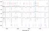 |
Fig. 2 Sample GOSSS spectra of LS III +46 11 and LS III +46 12 in the classical blue-violet spectral classification range. The top spectrum shows an example of LS III +46 11 near maximum velocity separation, the middle one an example of LS III +46 11 near minimum velocity separation, and the bottom one an example of LS III +46 12. The three cases show WHT data with the original spectral resolving power. |
The top two plots of Figs. 2 and 3 show two GOSSS spectra of LS III +46 11, one near maximum velocity separation and one close to the point where both stars have the same velocity. In the first plot, the spectra of the two components are virtually indistinguishable, with all the relevant stellar lines showing very similar ratios and widths. The only difference can be seen in the different absolute depths, those of the primary being ∼10% more intense than those of the secondary. Therefore, we assign the same spectral type to both components.
We classified the spectra using MGB (Maíz Apellániz et al. 2012) and v2.0 of the GOSSS standard grid (Maíz Apellániz et al. 2015). In the middle plot of Fig. 2, He iλ4471.507 appears as a very weak line in comparison with He iiλ4541.59, and N ivλ4057.75 is in emission with a similar intensity to N iiiλ4640.64+4641.85, indicating a spectral type of O3.5 (Walborn et al. 2002). He iiλ4685.71 has a P-Cygni profile3 (which appears to be present in both components, see the top plot) yielding a luminosity class of I since II is not defined at O3.5. Therefore, given the required f suffix (Table 2 in Sota et al. 2014), LS III +46 11 is an O3.5 If* + O3.5 If*.
The bottom plot of Fig. 2 shows a GOSSS spectrum of LS III +46 12. All the GOSSS spectra are consistent with a constant spectral type, i.e., we detect no sign of the target being an SB2. The GOSSS spectra are not calibrated in absolute velocity (the spectra are left in the star reference frame), but a comparison with prominent ISM lines shows no sign of relative velocity shifts, so we do not detect an SB1 character for LS III +46 12 either.
N ivλ4057.75 is not seen in emission in the spectrum of LS III +46 12 and He iλ4471.507 is significantly stronger than in LS III +46 11, yielding a spectral type of O4.5. He iiλ4685.71 is quite deep, so the luminosity class is V. Since N iiiλ4640.64+4641.85 is clearly in emission, C iiiλ4647.419+4650.246+4651.473 is weak, and there are no signs of line broadening, the final spectral type is O4.5 V((f)).
We note that N ivλ5200.41+5204.28+5205.15 is seen in absorption in all cases, as expected for these spectral types (Gamen & Niemelä 2002).
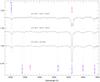 |
Fig. 3 Same as Fig. 2 for the wavelength range around He iiλ5411.53, the primary line we use for the stellar velocity measurements. |
3.2. Spectroscopic orbit of LS III +46 11
Most spectroscopic orbits for OB stars are studied with He i lines (or even with metallic lines for B stars) because they are intrinsically narrower than He ii lines. However, for a system composed of two O3.5 stars He i lines are not practical because they are too weak and we are forced to resort to the broader He ii lines4. The strongest He ii optical absorption lines in an O3.5 If* are He iiλ4541.591 and He iiλ5411.53. The large extinction experienced by LS III +46 11 (see below) makes a given S/N easier to attain with the latter than with the former, so we selected He iiλ5411.53 as our primary line. We note, however, that the CAHA-3.5 m spectra do not include it. In those cases we used He iiλ4541.591 instead for measuring Δv ≡ v2 − v1, the velocity difference between the primary and the secondary. We also note that the CAHA-3.5 m and OSN-1.5 m spectra were not calibrated in absolute velocity and that the WHT spectra were calibrated using ISM lines (instead of the lamps) present in both the WHT and the high-resolution spectra (which were calibrated using lamps).
All the epochs were fitted simultaneously with an IDL code by leaving the intensity and width of each component fixed (allowing for the different resolutions of each spectrograph) and fitting a four-component Gaussian for He iiλ5411.53 (the two stellar components plus the two DIBs at 5404.56 Å and 5418.87 Å, with the DIBs fixed at the same velocity for all epochs) and a two-component Gaussian for He iiλ4541.591. The initial period search was conducted using an IDL implementation of the information entropy algorithm of Cincotta et al. (1995). The orbit fitting itself (including the final period calculation) was done independently by two of us: J.M.A. used a code that he developed himself with the help of a previous routine written by R.C.G., and R.H.B. used an improved version of the Bertiau & Grobben (1969) code. The results were compared and found to be compatible, so only the first fitting will be reported here.
LS III +46 11 spectroscopic binary results for Δv ≡ v2 − v1. K12 is the radial velocity amplitude of the relative orbit.
LS III +46 11 spectroscopic binary results for v1 + v2. K1 and K2 are the radial velocity amplitudes of each orbit.
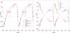 |
Fig. 4 Phased radial velocity curves for Δv (left) and v1 + v2 (right). The color code identifies the telescope. The left plot includes all data points, while the right plot excludes the two telescopes without accurate absolute velocity calibration (CAHA-3.5 m and OSN-1.5 m). |
A first analysis was carried out with Δv ≡ v2 − v1 and all the observations in Table 2. The results are given in Table 4 and plotted in the left panel of Fig. 4. In some cases with Δv close to zero it is not possible to identify which component was the one with the larger velocity since the two components are blended into a single Gaussian and, given the similar fluxes, switching them around does not appreciably change the reduced χ2 or  of the fit. For the epochs with identification confusion we used a Δv of zero with large error bars. The orbit obtained with Δv has a good fit ( = 1.43), a period consistent with the initial estimate, a relatively large eccentricity (as expected), and a very large minimum system mass (uncorrected for inclination) of 74.9 M⊙.
A second analysis was carried out with the separate v1 and v2 measurements. For this second analysis we excluded the CAHA-3.5 m spectra (for which we only had He iiλ4541.591 and were not calibrated in absolute velocity), the OSN-1.5 m spectra (also uncalibrated in absolute velocity and with identification confusion in all cases since we always caught LS III +46 11 near Δv = 0 with that configuration), and the WHT spectra with identification confusion. The results are listed in Table 5 and plotted in the right panel of Fig. 4. The value of is even better than for the first analysis and the results are generally compatible. The uncertainties of P, T0, e, and ω are slightly larger owing to the exclusion of some epochs. The mass ratio is close to the intensity ratio of the He iiλ5411.53 or He iiλ4541.59 lines and in the same sense: the component with the stronger lines is the most massive.
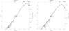 |
Fig. 5 Best SED CHORIZOS fits for LS III +46 11 (left, luminosity class of 1.0) and LS III +46 12 (right, luminosity class of 5.0). Blue data points are used for the input photometry (vertical error bars indicate photometric uncertainties, horizontal ones approximate filter extent) and green stars for the synthetic photometry. |
The values of γ1 and γ2 in Table 5 indicate that the LS III +46 11 center-of-mass radial velocity is in the range between −21 km s-1 and −17 km s-1 using the He iiλ5411.53 line. Fitting Gaussians to the LS III +46 11 high-resolution spectra with better S/N and lowest velocity separation also yield values in that range. However, doing the same with other lines gives different values: −27 ± 2 km s-1 for He iλ5875.65, −23 ± 4 km s-1 for O iiiλ5592.25, and −11 ± 3 km s-1 for He iiλ8236.79. These discrepancies are not uncommon when analyzing early-type O stars owing to the intrinsic width of their lines and the effect of winds. We can conclude that the true center-of-mass radial velocity of LS III +46 11 is between −25 km s-1 and −15 km s-1 without being able to provide a more precise measurement at this time.
We also analyzed the velocity of LS III +46 12 using the four high-resolution epochs listed in Table 3. We were unable to detect clear radial velocity variations at a level of 10 km s-1 or higher, but with such a small number of epochs it is not possible to ascertain the spectroscopic binarity of the system. We measured the radial velocity of the system using the same four spectral lines as for LS III +46 11 and obtained a smaller range between −16 km s-1 and −10 km s-1. The better agreement between lines is possibly caused by the weaker winds in the dwarf compared to the supergiant pair. These results are consistent with LS III +46 12 being a spectroscopic single with the same center-of-mass radial velocity as LS III +46 11 because the stronger winds of the latter likely bias its measured velocity towards more negative (blueshifted) values. In addition, the experience with LS III +46 11 and other systems indicates that we should not exclude the possibility of LS III +46 12 being a spectroscopic system with a period of months or longer.
3.3. CHORIZOS analysis of LS III +46 11 and LS III +46 12
We processed the Johnson+Tycho+2MASS photometry of LS III +46 11 and LS III +46 12 using the latest version of the CHORIZOS code (Maíz Apellániz 2004) to determine the amount and type of extinction and the distance to the stars. The CHORIZOS runs were executed with the following conditions:
-
We used the Milky Way grid ofMaíz Apellániz (2013b), in whichthe two grid parameters are effective temperature (Teff) andphotometric luminosity class (LC). The latter quantity is definedin an analogous way to the spectroscopic equivalent, but insteadof being discrete it is a continuous variable that varies from 0.0(highest luminosity for that Teff) to 5.5 (lowest luminosity for that Teff).We note that the range is selected in order to make objects withspectroscopic luminosity class V (dwarfs) haveLC ≈ 5 and objects with spectral luminosity class I have LC ≈ 1. For O stars the spectral energy distributions (SEDs) are TLUSTY (Lanz & Hubeny 2003).
-
The extinction laws were those of Maíz Apellániz et al. (2014), which are a single-family parameter with the type of extinction defined by R5495. The amount of extinction is parameterized by E(4405 − 5495). See Maíz Apellániz (2013a) for their relationship with RV and E(B − V) and why those quantities are not good choices to characterize extinction.
-
The Teff-spectral type conversion used is an adapted version of Martins et al. (2005) that includes the spectral subtypes used by Sota et al. (2011, 2014).
-
Teff and LC were fixed while R5495, E(4405 − 5495), and log d were left as free parameters. The values of the Teff were established from the used Teff-spectral type conversion (see previous point). For LC we explored a range of possible values by doing CHORIZOS runs with 0.0, 0.5, 1.0, 1.5, and 2.0 for LS III +46 11 and runs with 4.0, 4.5, 5.0, and 5.5 for LS III +46 12.
The CHORIZOS results are shown in Table 6 and the best SEDs are plotted in Fig. 5 along with the input and synthetic photometry.
Results of the CHORIZOS fits for LS III +46 11 and LS III +46 12.
AstraLux results for LS III +46 11 and LS III +46 12.
2MASS photometry for the targets detected in the AstraLux images. ABC flags are used for normal detections (with increasingly larger uncertainties), U flags for upper limits on magnitudes, and T for measurements done in this work.
-
As expected, the different runs for a given star with different val-ues of LC give nearly identical results for
, R5495, and E(4405 − 5495) andonly differ in log d. This happens because the optical+NIR colors ofO stars are nearly independent of luminosity5 for a fixed Teff. Therefore, here we concen-trate on the results for LC = 1.0(LS III +46 11)and LC = 5.0(LS III +46 12)and consider the other runs only when discussing the distance. -
The values of
indicate that the fit is good, even for two cases such as these where the extinction is considerable. We also ran alternative CHORIZOS executions using the Cardelli et al. (1989) and Fitzpatrick (1999) extinction laws. For Cardelli et al. (1989) the were similar, as expected for stars with moderate extinction with broad-band photometry and R5495 values close to the canonical 3.1. For Fitzpatrick (1999) the were significantly worse (by a factor of ≈2). Therefore, these results are another sign of the validity of the Maíz Apellániz et al. (2014) extinction laws for Galactic targets. -
The two stars show values of R5495 that are compatible and only slightly larger than the canonical value of 3.1. Therefore, the same type of dust appears to lie between each star and us and the grain size is typical for the Milky Way.
-
The LS III +46 11 extinction is significantly higher than that of LS III +46 12, which explains the similar magnitudes of the two objects even though LS III +46 11 is expected to be intrinsically more luminous and located at the same distance. This result also implies that there is significant differential extinction within the Berkeley 90 field. The value of E(4405 − 5495) for LS III +46 12 is close to the E(B − V) = 1.15 result for Berkeley 90 of Tadross (2008).
-
The values for log d listed are the uncorrected CHORIZOS output and are equivalent to spectroscopic parallaxes. They do not take into account that LS III +46 11 is an SB2 system with two components with similar luminosities while LS III +46 12 is apparently single. Therefore, the log d values for LS III +46 11 have to be increased by ≈
 . This implies that the derived distances for LS III +46 11 and LS III +46 12 are incompatible. Another way to look at the discrepancy is that if we use the extinction-corrected apparent Johnson V magnitude (VJ,0) for LS III +46 11 and apply a ≈2.5log 2 = 0.753 correction, we end up with two stars with VJ,0 values between 6.1 and 6.2, not brighter but actually slightly fainter than LS III +46 12. In other words, if the three stars are at the same distance, we would require the two objects with spectroscopic class I to be fainter than the object with spectroscopic class V. We analyze the distance question later on.
3.4. Visual multiplicity
Table 7 gives the separation, orientation, and magnitude difference between the brightest star in the AstraLux Norte images (either LS III +46 11 or LS III +46 12) and the rest of the detected point sources. We note that the AstraLux images are not absolutely calibrated, so only differential photometry is provided; hence, all the data refer to stellar pairs. Nevertheless, the photometry in the i and z bands for the two bright stars can be derived from the best SED in the previous subsection: LS III +46 11 A has zero-point-corrected AB i and z magnitudes of 9.549 and 9.017, respectively, and LS III +46 12 A has zero-point-corrected AB i and z magnitudes of 9.371 and 9.043, respectively. Table 8 gives the 2MASS JHKS magnitudes for the stars in the AstraLux images. All are detected except for LS III +46 11 F, the dimmest star in the AstraLux image. We note that the 2MASS magnitudes are not complete, as usual for moderately crowded fields such as this one.
The most relevant result is that LS III +46 11 has no visual companions within 11′′ and that LS III +46 12 has just one dim companion 6′′ away. From the photometric point of view, this means that the analysis in the previous section does not appear to include additional stars, so one can refer to the photometry of LS III +46 11 and LS III +46 11 A as indistinguishable6 (as we have done in the previous paragraph) and the same can be said about LS III +46 12 and LS III +46 12 A. From the physical point of view, this means that (barring any undetected components) LS III +46 11 is a double system but likely not a higher-order one, since F or C (the closest companions) are likely to be unbound, especially considering that their environment is the center of a cluster. On the other hand, LS III +46 12 B is ∼10 000 AU in the plane of the sky away from A and could possibly be bound (Maíz Apellániz 2010). There is also another component visible in the 2MASS images (but not listed in Tables 7 or 8 because it fell just outside the 25″ × 25″ AstraLux Norte field of view) 7′′ to the east of LS III +46 12 A, thus increasing the probability of the existence of a bound companion.
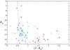 |
Fig. 6 2MASS CMD for stars within 3′ of the nominal center of Berkeley 90 passing the cuts described in the text. The blue circles are all the stars with 0.45 < (J − KS) < 0.9. Red-star symbols are used to mark stars with Hα emission, as selected from Fig. 7. The thick line is a 2 Ma isochrone with high rotation from Ekström et al. (2012) displaced to DM = 12.0 (log d = 3.4) with E(J − KS) = 0.75. The brightest objects are LS III +46 11 (to the right of the isochrone) and LS III +46 12 (to the left). |
3.5. Berkeley 90 photometry
The area of Berkeley 90 is immersed in bright nebulosity (Sh 2-115, Sharpless 1959), indicating the existence of sources with large ionizing fluxes, but the cluster has surprisingly received very little attention. We have used photometric data from 2MASS (Skrutskie et al. 2006) and IPHAS (Barentsen et al. 2014) to study its properties. We have selected 2MASS sources within 3′ of the nominal center of the cluster, as given in SIMBAD. We have rejected stars with bad quality flags, and cross-matched our selection with the IPHAS catalogue. As the IPHAS catalogue contains many spurious sources in areas of bright nebulosity, we have only accepted sources with a 2MASS counterpart within a  radius. The QIR parameter, defined as QIR = (J − H) − 1.8 × (H − KS), is very effective at separating early- and late-type stars (e.g., Comerón & Pasquali 2005; Negueruela & Schurch 2007), with early-type stars showing values ≈0.0. We select objects with QIR< 0.08 as candidate early-type stars (see Negueruela & Schurch 2007), though emission-line stars also display negative values due to their KS excesses. The candidates are clearly concentrated towards the cluster center, confirming that they mainly represent the cluster population. The KS/ (J − KS) diagram for the resulting selection is shown in Fig. 6.
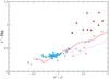 |
Fig. 7 IPHAS (r′ − i′)/(r′ − Hα) diagram. The solid (red) line is the locus of the main sequence for E(4405 − 5495) = 1 from Drew et al. (2005), while the (magenta) dotted line is the locus of the main sequence for E(4405 − 5495) = 2, roughly defining the envelope for the hot stars that are cluster members. Blue circles are used to indicate the stars selected from Fig. 6 and marked in the same way there. Since all the stars have been selected to have a pseudocolor QIR typical of early-type stars or emission-line stars and they all have relatively red (J − KS) colors, we can safely assume that stars clearly above the main-sequence locus are emission-line stars. Their positions in the 2MASS CMD, (red stars here and in Fig. 6), are in all cases compatible with this interpretation. Both LS III +46 11 and LS III +46 12 are saturated in IPHAS, as all bright O stars in the northern sky are. |
Possible cluster members show a broad distribution in (J − KS). Three objects with (J − KS) < 0.4 are located away from the cluster and may be foreground stars. Interestingly, LS III +46 12 has the second lowest (J − KS) of all possible members, with 0.46 ± 0.03, while the location of LS III +46 11 in Fig. 6 shows that it is more reddened (as we already knew from the CHORIZOS analysis). We assume that the bulk of cluster members is given by the vertical strip extending between (J − KS) = 0.45 and (J − KS) = 0.9. This is confirmed by their concentration in the IPHAS (r′ − i′)/(r′ − Hα) diagram (Fig. 7), where all except three are distributed in a narrow strip with 0.7 ≲ (r′ − i′) ≲ 1.05 that follows the reddening vector, and the vast majority have 0.8 ≲ (r′ − i′) ≲ 1.0. The main concentration of cluster members, lying between LS III +46 11 and LS III +46 12, shows only a small spread in color, while the stars lying immediately adjacent to LS III +46 11 both to the north and west display higher values. The average (J − KS) for all stars with values between 0.45 and 0.9 is 0.67 with a standard deviation σ = 0.12, which shows that the objects are evenly distributed between these values; therefore, defining a typical reddening for the cluster is meaningless.
A significant number of sources occupy positions in the (r′ − i′)/(r′ − Hα) diagram compatible with emission-line stars, displaying (r′ − Hα) > 0.8 and (r′ − i′) > 1.2 (Corradi et al. 2008). Almost all these objects are quite faint and display high values of (J − KS) > 1.4. More than half have QIR< − 0.1, typical of emission line stars. These objects can represent a population of pre-main sequence stars associated with the cluster. Interestingly, none of them is located in the central region of the cluster.
As there are no obviously evolved stars, it is not possible to assign an age to Berkeley 90. We note that the luminosity difference between dwarfs and supergiants is relatively small at the earliest spectral types. Assuming that LS III +46 12 is slightly evolved, we can perhaps give an age ∼2 Ma, but luminous O-type stars in Cygnus OB2 with spectral types O3-O5 are significantly hotter than the main-sequence turn-off (Negueruela et al. 2008). By analogy, an age of up to 3 Ma is possible. As an illustration, Fig. 6 shows a high-rotation isochrone from Ekström et al. (2012) corresponding to an age of 2 Ma, reddened by a representative E(J − KS) = 0.75 and displaced to DM = 12.0 mag (log d = 3.4). The fit to the position of objects in the central concentration is rather good, considering the variable reddening. Three objects lie well to the left of the isochrone and therefore are either non-members or outliers with low reddening. All of them lie to the east of LS III +46 12, except one that is located at the northern edge of the region analyzed. However, removing these objects does not change the average color or its standard deviation. On the other hand, a few objects lying to the right of the isochrone, with (J − KS) ≈ 1.0 are likely cluster members with higher than average reddening.
In spite of the presence of three early O-type stars (two in LS III +46 11 and at least one in LS III +46 12), Berkeley 90 seems to contain very few OB stars. Only one photometric member is sufficiently bright in KS to be a late-O star, 2MASS J20350798+4649321 (Fig. 1), and this object has a position in the IPHAS diagrams consistent with being an emission-line star (it is the object indicated by both a blue circle and a red-star symbol in Figs. 6 and 7). The bulk of the population starts almost 3 mag below LS III +46 12, at KS ≈ 10.5, an intrinsic magnitude roughly corresponding to a B1 V spectral type.
4. Discussion
O stars earlier than type O4 are very scarce in the Galaxy. Prior to this work, there were only two examples known in the northern hemisphere, Cyg OB2-7 and Cyg OB2-22 A (Walborn et al. 2002; Sota et al. 2011). Given that we know so few very massive stars, it is crucial to keep searching for them to increase our statistics if we want to establish what is the stellar upper mass limit and its dependence on metallicity and environmental conditions.
We have shown that LS III +46 11 is a very massive eccentric binary composed of two near-twin stars. A few years ago this may have been seen as a fluke, but several similar systems have recently been discovered.
-
HD 93 129 AaAb(Nelan et al. 2004, 2010; Maíz Apellánizet al. 2005, 2008; Sotaet al. 2014) may be evenmore massive, given that the primary is of spectral typeO2 If*, but the secondary is one magnitude fainterand the orbit is yet undetermined and appears to be decades tocenturies long.
-
Cyg OB2-9 (Nazé et al. 2012, O5-5.5 I + O3-4 III) has a very similar mass ratio and a somewhat larger eccentricity, its (M1 + M2)sin3i is only slightly lower, its period is an order of magnitude larger, and the spectral types are slightly later.
-
R139 (Taylor et al. 2011, O6.5 Iafc + O6 Iaf) is also similar to LS III +46 11 in terms of period, eccentricity, and mass ratio, but the two stars are mid-O supergiants and their lower mass limits are significantly higher, between 60 and 80 M⊙. These masses indicate that not all objects above 60 M⊙ are WNh stars (of course, as long as we do not know the inclinations in this and other cases, we will not know what the true masses are).
-
Two additional examples of very massive stars in elliptical orbits whose large eccentricity made the discovery of their binarity difficult are WR 22 ≡ HD 92 740 (Moffat & Seggewiss 1978; Conti et al. 1979; Schweickhardt et al. 1999, WN7 + O8-9.5 III:) and HD 93 162 (Gamen et al. 2008; Sota et al. 2014, O2.5 If*/WN6 + OB).
-
There are also very massive twin systems in shorter, near-circular orbits such as NGC 3603-A1 (Moffat et al. 2004; Schnurr et al. 2008, WN6ha + WN6ha), WR 20a (Rauw et al. 2004; Bonanos et al. 2004; Crowther & Walborn 2011, O3 If*/WN6 + O3 If*/WN6), and Pismis 24-1 (Maíz Apellániz et al. 2007, O3.5 If* + O4 III(f) + ...). The last of these also includes a third very massive component in a long orbit.
-
All of these systems are located in regions with large numbers of O stars (Carina Nebula; Cygnus OB2; 30 Doradus; NGC 3603; Westerlund 2; and, to a lesser extent, Pismis 24). LS III +46 11 is the oddity because it is located in a significantly less massive cluster or association. In this respect, a more similar case may be HD 150 136, which is apparently less evolved but is a triple system [O3-3.5 V((f*)) + O5.5-6 V((f)) + O6.5-7 V((f))] with a most massive star of 53 ± 10 M⊙ in a relatively small cluster, NGC 6193, with another nearby star, HD 150 135 [O6.5 V((f))z], yielding a similar makeup to that of Berkeley 90 (Niemelä & Gamen 2005; Mahy et al. 2012; Sana et al. 2013b; Sánchez-Bermúdez et al. 2013; Sota et al. 2014).
All of the cases mentioned above refer to distant very massive stars (Cyg OB2-9 and HD 150 136 are the closest, but they are beyond 1 kpc), but what is even more surprising is the recent discovery that some of the brightest and closest O stars in the sky have eccentric companions. That is what has happened with θ1 Ori C (Kraus et al. 2007; Sota et al. 2011, O7 Vp + ...) and σ Ori A (Simón-Díaz et al. 2011, 2015a, O9.5 V + B0/1 Vn; we note that σ Ori B is B0.5 V). Why were these systems not discovered earlier? There are two reasons: eccentric systems require extensive spectroscopic monitoring since their velocity differences may be too small to be detected during a large fraction of their orbits (as happened with LS III +46 11) and in some cases interferometry is the only way to detect their multiplicity because of their large semi-major axes. It was not until the last decade that large-scale spectroscopic monitoring of many O stars started and that interferometric technology allowed similar surveys using those techniques. However, many systems still remain outside the reach of such surveys so discoveries should continue in the following years.
Our data cannot provide conclusive results on the masses of LS III +46 11 and LS III +46 12. Without eclipses, we cannot accurately measure the inclination of the LS III +46 11 orbit and our Keplerian masses of 38.80 ± 0.83 M⊙ and 35.60 ± 0.77 M⊙ have the sin3i factor included in them, making them just lower limits. We note that the star is not present in the public release of the Northern Sky Variability Survey (Woźniak et al. 2004) and that the time coverage in the SuperWASP (Pollacco et al. 2006) public archive is very limited, so a thorough search for eclipses is not possible at this time. In any case, eclipses are unlikely, since the large separations in the orbit would require an inclination very close to 90 degrees in order for them to take place. The inclination could be constrained in the future with broadband polarimetry or through the phase-dependent behavior of excess emission from colliding winds.
For evolutionary masses, we have a different problem: our results for the spectral types and distances are inconsistent. There are three possible explanations:
-
1.
A straightforward interpreta-tion of the CHORIZOS results placeLS III +46 11 ata log d between 3.45 and 3.67(in parsecs, after cor-recting for the existence of two stars) andLS III +46 12 ata log d between 3.10 and 3.28. Therefore, one possi-bility would be that both objects are physically unrelated andjust the result of a chance alignment. In this case, the luminosityclassification criteria for early-type O stars would retain theirphysical meaning and there would be no need to invoke the exis-tence of undetected multiple systems. Nevertheless, we judgethis possibility to be highly unlikely, given the small number ofearly-type O stars that exist and the existence of the underlyingcluster Berkeley 90. This hypothesis will be testedsoon once the Gaia parallaxes become available.
-
2.
An alternative interpretation would place both LS III +46 11 and LS III +46 12 at a log d∼ 3.4, consistent with the 2MASS photometry of Berkeley 90, but would require that the current luminosity classification criteria for O stars based on the depth of He iiλ4685.71 does not really reflect a function or luminosity, but instead is just a measurement of wind strength7. We consider this option unlikely as there are both theoretical reasons why (for the same Teff and metallicity) wind strength should strongly correlate with luminosity and observational data that corroborate that association (e.g., Walborn et al. 2014). This hypothesis could be tested by obtaining a good S/N high-resolution spectrum of LS III +46 12 and modeling it, for example with FASTWIND or CMFGEN. Those codes derive gravity from a fit to the Balmer line profiles, so He iiλ4685.71 does not affect the result.
-
3.
A third option is that LS III +46 12 is another near-twin binary system composed of two very-early-type O dwarfs. In this scenario, log d would be in the 3.40-3.45 range, marginally consistent with the spectroscopic parallaxes for LS III +46 11 and Berkeley 90. This solution may be ad hoc, but we believe it to be the most likely one. Indeed, there is a precedent with an object that is a near-spectroscopic twin of LS III +46 12, HD 93 250 (O4 III(fc), Sota et al. 2014). Its spectroscopic parallax was incompatible with the well-known value of the Carina Nebula until it was discovered to be a binary through interferometry (Sana et al. 2011). We note that there is a large range of parameter space for which we would not detect significant velocity variations if the system were a binary, especially considering that our spectroscopic campaign was not as thorough for LS III +46 12 as it was for LS III +46 11. For example, the period could be of the order of decades or centuries or the inclination could be small. Also, X-ray excesses due to wind-wind collisions are expected to be weaker for dwarfs than for supergiants.
Related to the issue of the masses is the age of Berkeley 90. Until one of the above explanations is confirmed, we cannot provide a final answer. We should note, however, that if the third option is the correct one, it is possible to derive a consistent age of 1.5–2.0 Ma for LS III +46 11, LS III +46 12, and Berkeley 90 using the low-rotation Geneva evolutionary tracks of Lejeune & Schaerer (2001). Under these assumptions, the masses of the two stars in LS III +46 11 would be in the 60–70 M⊙ range and those in LS III +46 12 would be 35–45 M⊙.
The results in this paper reveal that Berkeley 90 can be an important cluster with which to resolve the issue of how the stellar initial mass function (IMF) is sampled. There are two alternative theories, one that states that the IMF is built in a sorted way, with many low-mass stars being formed before any high-mass star can appear, and another that states that the IMF is built in a stochastic way, with some rare cases where it is possible to form high-mass stars with a relatively small number of low-mass ones (see Bressert et al. 2012 and references therein). If the third option on the LS III +46 11 and LS III +46 12 masses above is correct, we would have a cluster with four stars above 35 M⊙, one of them with ∼70 M⊙, and none or just one (2MASS J20350798+4649321) between 20 and 35 M⊙ (see Fig. 6 and the associated discussion in the text). Using the total stellar mass above 20 M⊙ and assuming a Kroupa IMF (Kroupa 2001) between 0.1 M⊙ and 100 M⊙, we derive that the mass of Berkeley 90 is ≈2000 M⊙, which is consistent with the appearance of the cluster in relationship with other similar objects. However, such a large maximum stellar mass in such a small cluster could be incompatible with the sorted sampling scenario (Weidner & Kroupa 2006) but can be accomodated within the stochastic scenario: a 2000 M⊙ cluster with the conditions above should have, on average, 2.3 stars in the 20–35 M⊙ range and 1.6 stars in the 35–100 M⊙ range. We observe 1 star in the first range and 4 in the second, i.e., off from the expected values but within the range of possibilities expected for a single case within the number of similar clusters in the solar neighborhood. We need better data (constraining the nature of LS III +46 12 with interferometry, studying a deep CMD of Berkeley 90 to accurately measure the cluster mass, and resolving the distance issues with Gaia) to provide a final answer, but Berkeley 90 appears to be a good candidate for a small cluster with a star too massive for the sorted sampling scenario.
5. Conclusions
-
Berkeley 90 is a youngstellar cluster dominated by two early O-type systems.LS III +46 11 isan SB2 composed of two very sim-ilar O3.5 If* stars.LS III +46 12 isspectroscopically single and has a spectral typeO4.5 V((f)).
-
LS III +46 11 has an eccentric orbit (e between 0.56 and 0.57) with a 97.2-day period and minimum masses of 38.80 ± 0.83 M⊙ and 35.60 ± 0.77 M⊙. Since we do not know the inclination we cannot calculate accurate Keplerian masses.
-
LS III +46 11 has a significantly higher extinction than LS III +46 12. The optical+NIR extinction law is close to the average one in the Galaxy.
-
There are no apparent bright visual companions to either system.
-
The evolutionary masses of LS III +46 11 and LS III +46 12 are incompatible with the two systems being located at the same distance and having the same age. We consider different solutions to the problem and consider that the most likely one is the existence of an undetected companion for LS III +46 12, for which there is plenty of room in terms of period, inclination, and eccentricity not yet explored.
-
Berkeley 90 is a cluster with considerable differential extinction and its stellar mass is possibly too low to harbor both LS III +46 11 and LS III +46 12 under the sorted sampling scenario for the IMF.
The GOSSS spectra shown in Sota et al. (2011, 2014) have been homogenized to R = 2500 whenever the resolving power was slightly higher.
Throughout this work we refer to each line with the exact rest wavelength we are using in order to avoid problems with future comparisons of absolute velocity values. The different number of significant digits reflects the uncertainty in our knowledge of the rest wavelengths and/or the singlet/multiplet nature.
The absorption component is only slightly blueshifted.
This is a factor that likely contributed to the previous failure of the detection of the SB2 character of LS III +46 11.
The largest difference takes place in the KS band and is due to the wind contribution, but that effect is not taken into account in the TLUSTY SEDs and is only expected to be on the order of 0.01 magnitudes for the cases of interest here.
LS III +46 11 A includes two spectroscopic components, but their separation, as previously derived, is on the order of 1 mas, i.e., two orders of magnitude below the value that can be resolved with AstraLux Norte. See Fig. 2 in Maíz Apellániz (2010) for the values of separations and magnitude differences that AstraLux Norte can resolve.
The continuum of LS III +46 12 to the right of He iiλ4685.71 is slightly raised, possibly signaling an anomalous profile indicative of luminosity class III rather than V, which would have a similar effect to the one described here.
Acknowledgments
We thank the referee, Tony Moffat, for his useful comments that helped improve this paper. J.M.A. and A.S. acknowledge support from [a] the Spanish Government Ministerio de Economía y Competitividad (MINECO) through grants AYA2010-15 081, AYA2010-17 631, and AYA2013-40 611-P and [b] the Consejería de Educación of the Junta de Andalucía through grant P08-TIC-4075. J.M.A. was also supported by the George P. and Cynthia Woods Mitchell Institute for Fundamental Physics and Astronomy and he is grateful to the Department of Physics and Astronomy at Texas A&M University for their hospitality during some of the time this work was carried out. I.N., A.M., J.A., and J.L. acknowledge support from [a] the Spanish Government Ministerio de Econoía y Competitividad (MINECO) through grant AYA2012-39 364-C02-01/02, [b] the European Union, and [c] the Generalitat Valenciana through grant ACOMP/2014/129. R.H.B. acknowledges support from FONDECYT Project 1 140 076. S.S.-D. acknowledges funding by [a] the Spanish Government Ministerio de Economía y Competitividad (MINECO) through grants AYA2010-21 697-C05-04, AYA2012-39 364-C02-01, and Severo Ochoa SEV-2011-0187 and [b] the Canary Islands Government under grant PID2 010 119. J.S.-B. acknowledges support by the JAE-PreDoc program of the Spanish Consejo Superior de Investigaciones Científicas (CSIC). STScI is operated by the Association of Universities for Research in Astronomy, Inc., under NASA contract NAS5-26555.
References
- Barbá, R. H.,Gamen, R. C.,Arias, J. I., et al. 2010, Rev. Mex. Astron. Astrofís. Conf. Ser., 38, 30 [Google Scholar]
- Barentsen, G.,Farnhill, H. J.,Drew, J. E., et al. 2014, MNRAS, 444, 3230 [NASA ADS] [CrossRef] [Google Scholar]
- Bertiau, F. C., &Grobben, J. 1969, Ricerche Astronomiche, 8, 1 [Google Scholar]
- Bonanos, A. Z.,Stanek, K. Z.,Udalski, A., et al. 2004, ApJ, 611, L33 [NASA ADS] [CrossRef] [Google Scholar]
- Bressert, E.,Bastian, N.,Evans, C. J., et al. 2012, A&A, 542, A49 [NASA ADS] [CrossRef] [EDP Sciences] [Google Scholar]
- Cardelli, J. A.,Clayton, G. C., &Mathis, J. S. 1989, ApJ, 345, 245 [NASA ADS] [CrossRef] [Google Scholar]
- Cincotta, P. M.,Méndez, M., &Núñez, J. A. 1995, ApJ, 449, 231 [NASA ADS] [CrossRef] [Google Scholar]
- Comerón, F., &Pasquali, A. 2005, A&A, 430, 541 [NASA ADS] [CrossRef] [EDP Sciences] [Google Scholar]
- Conti, P. S.,Niemelä, V. S., &Walborn, N. R. 1979, ApJ, 228, 206 [NASA ADS] [CrossRef] [Google Scholar]
- Corradi, R. L. M.,Rodríguez-Flores, E. R.,Mampaso, A., et al. 2008, A&A, 480, 409 [NASA ADS] [CrossRef] [EDP Sciences] [Google Scholar]
- Crowther, P. A., &Walborn, N. R. 2011, MNRAS, 416, 1311 [NASA ADS] [CrossRef] [MathSciNet] [Google Scholar]
- Crowther, P. A.,Schnurr, O.,Hirschi, R., et al. 2010, MNRAS, 408, 731 [NASA ADS] [CrossRef] [Google Scholar]
- Drew, J. E.,Greimel, R.,Irwin, M. J., et al. 2005, MNRAS, 362, 753 [NASA ADS] [CrossRef] [Google Scholar]
- Ekström, S.,Georgy, C.,Eggenberger, P., et al. 2012, A&A, 537, A146 [NASA ADS] [CrossRef] [EDP Sciences] [Google Scholar]
- Fitzpatrick, E. L. 1999, PASP, 111, 63 [NASA ADS] [CrossRef] [Google Scholar]
- Gamen, R., & Niemelä, V. S. 2002, in Rev. Mex. Astron. Astrofís. Conf. Ser. 14, eds. J. J. Claria, D. García Lambas, & H. Levato, 16 [Google Scholar]
- Gamen, R. C.,Gosset, E.,Morrell, N. I., et al. 2008, Rev. Mex. Astron. Astrofís. Conf. Ser., 33, 91 [Google Scholar]
- Gardini, A., Maíz Apellániz, J., Pérez, E., Quesada, J. A., & Funke, B. 2013, in Highlights of Spanish Astrophysics VII, Proc. X Sci. Meet. SAS, 947 [Google Scholar]
- Hardorp, J., Theile, I., & Voigt, H. H. 1964, Hamburger Sternw. Warner & Swasey Obs., 3 [Google Scholar]
- Harten, R., &Felli, M. 1980, A&A, 89, 140 [NASA ADS] [Google Scholar]
- Høg, E.,Fabricius, C.,Makarov, V. V., et al. 2000, A&A, 355, L27 [NASA ADS] [Google Scholar]
- Kraus, S.,Balega, Y. Y.,Berger, J.-P., et al. 2007, A&A, 466, 649 [NASA ADS] [CrossRef] [EDP Sciences] [Google Scholar]
- Kroupa, P. 2001, MNRAS, 322, 231 [NASA ADS] [CrossRef] [Google Scholar]
- Lanz, T., &Hubeny, I. 2003, ApJS, 146, 417 [NASA ADS] [CrossRef] [Google Scholar]
- Lejeune, T., &Schaerer, D. 2001, A&A, 366, 538 [NASA ADS] [CrossRef] [EDP Sciences] [Google Scholar]
- Mahy, L.,Gosset, E.,Sana, H., et al. 2012, A&A, 540, A97 [NASA ADS] [CrossRef] [EDP Sciences] [Google Scholar]
- Maíz Apellániz, J. 2004, PASP, 116, 859 [NASA ADS] [CrossRef] [Google Scholar]
- Maíz Apellániz, J. 2010, A&A, 518, A1 [NASA ADS] [CrossRef] [EDP Sciences] [Google Scholar]
- Maíz Apellániz, J. 2013a, in Highlights of Spanish Astrophysics VII, Proc. X Sci. Meet. SAS, 583 [Google Scholar]
- Maíz Apellániz, J. 2013b, in Highlights of Spanish Astrophysics VII, Proc. X Sci. Meet. SAS, 657 [Google Scholar]
- Maíz Apellániz, J., Úbeda, L., Walborn, N. R., & Nelan, E. P. 2005, in Resolved Stellar Populations, eds. D. Valls-Gabaud, & M. Chávez [arXiv:astro-ph/0506283] [Google Scholar]
- Maíz Apellániz, J.,Walborn, N. R.,Morrell, N. I.,Niemelä, V. S., &Nelan, E. P. 2007, ApJ, 660, 1480 [NASA ADS] [CrossRef] [Google Scholar]
- Maíz Apellániz, J.,Walborn, N. R.,Morrell, N. I., et al. 2008, Rev. Mex. Astron. Astrofís. Conf. Ser., 33, 55 [NASA ADS] [Google Scholar]
- Maíz Apellániz, J., Sota, A., Walborn, N. R., et al. 2011, in Highlights of Spanish Astrophysics VI, Proc. IX Sci. Meet. SAS, 467 [Google Scholar]
- Maíz Apellániz, J., Pellerin, A., Barbá, R. H., et al. 2012, in ASP Conf. Ser. 465, eds. L. Drissen, C. Robert, N. St.-Louis, & A. F. J. Moffat, 484 [Google Scholar]
- Maíz Apellániz, J., Alfaro, E. J., Arias, J. I., et al. 2015, in Highlights of Spanish Astrophysics VIII, Proc. XI Sci. Meet. SAS, 603 [Google Scholar]
- Maíz Apellániz, J.,Evans, C. J.,Barbá, R. H., et al. 2014, A&A, 564, A63 [NASA ADS] [CrossRef] [EDP Sciences] [Google Scholar]
- Martins, F.,Schaerer, D., &Hillier, D. J. 2005, A&A, 436, 1049 [NASA ADS] [CrossRef] [EDP Sciences] [Google Scholar]
- Mason, B. D.,Gies, D. R.,Hartkopf, W. I., et al. 1998, AJ, 115, 821 [NASA ADS] [CrossRef] [Google Scholar]
- Mayer, P., &Macák, P. 1973, Bull. Astr. Inst. Czechosl., 24, 50 [Google Scholar]
- Moffat, A. F. J., &Seggewiss, W. 1978, A&A, 70, 69 [NASA ADS] [Google Scholar]
- Moffat, A. F. J.,Poitras, V.,Marchenko, S. V., et al. 2004, AJ, 128, 2854 [NASA ADS] [CrossRef] [Google Scholar]
- Motch, C.,Haberl, F.,Dennerl, K.,Pakull, M., &Janot-Pacheco, E. 1997, A&A, 323, 853 [NASA ADS] [Google Scholar]
- Nazé, Y.,Mahy, L.,Damerdji, Y., et al. 2012, A&A, 546, A37 [NASA ADS] [CrossRef] [EDP Sciences] [Google Scholar]
- Negueruela, I., &Schurch, M. P. E. 2007, A&A, 461, 631 [NASA ADS] [CrossRef] [EDP Sciences] [Google Scholar]
- Negueruela, I.,Marco, A.,Herrero, A., &Clark, J. S. 2008, A&A, 487, 575 [NASA ADS] [CrossRef] [EDP Sciences] [Google Scholar]
- Negueruela, I., Maíz Apellániz, J., Simón-Díaz, S., et al. 2015, in Highlights of Spanish Astrophysics VIII, Proc. XI Sci. Meet. SAS, 524 [Google Scholar]
- Nelan, E. P.,Walborn, N. R.,Wallace, D. J., et al. 2004, AJ, 128, 323 [NASA ADS] [CrossRef] [Google Scholar]
- Nelan, E. P.,Walborn, N. R.,Wallace, D. J., et al. 2010, AJ, 139, 2714 [NASA ADS] [CrossRef] [Google Scholar]
- Niemelä, V. S., &Gamen, R. C. 2005, MNRAS, 356, 974 [NASA ADS] [CrossRef] [Google Scholar]
- Pellerin, A., Maíz Apellániz, J.,Simón-Díaz, S., &Barbá, R. H. 2012, AAS Meet. Abstr., 219, 224.03 [Google Scholar]
- Pollacco, D. L., Skillen, I., Collier Cameron, A., et al. 2006, PASP, 118, 1407 [NASA ADS] [CrossRef] [Google Scholar]
- Rauw, G., De Becker, M.,Nazé, Y., et al. 2004, A&A, 420, L9 [NASA ADS] [CrossRef] [EDP Sciences] [Google Scholar]
- Sana, H., Le Bouquin, J.-B., De Becker, M., et al. 2011, ApJ, 740, L43 [NASA ADS] [CrossRef] [Google Scholar]
- Sana, H., de Mink, S. E., de Koter, A., et al. 2012, Science, 337, 444 [Google Scholar]
- Sana, H., de Koter, A., de Mink, S. E., et al. 2013a, A&A, 550, A107 [NASA ADS] [CrossRef] [EDP Sciences] [Google Scholar]
- Sana, H., Le Bouquin, J.-B.,Mahy, L., et al. 2013b, A&A, 553, A131 [NASA ADS] [CrossRef] [EDP Sciences] [Google Scholar]
- Sánchez-Bermúdez, J.,Schödel, R.,Alberdi, A., et al. 2013, A&A, 554, L4 [NASA ADS] [CrossRef] [EDP Sciences] [Google Scholar]
- Sanduleak, N. 1974, PASP, 86, 74 [NASA ADS] [CrossRef] [Google Scholar]
- Schnurr, O., Casoli, J., Chené, A.-N., Moffat, A. F. J., & St.-Louis, N. 2008, MNRAS, 389, L38 [NASA ADS] [CrossRef] [Google Scholar]
- Schweickhardt, J.,Schmutz, W.,Stahl, O.,Szeifert, T., &Wolf, B. 1999, A&A, 347, 127 [NASA ADS] [Google Scholar]
- Sharpless, S. 1959, ApJS, 4, 257 [Google Scholar]
- Simón-Díaz, S., Castro, N., García, M., & Herrero, A. 2011, in IAU Symp. 272, eds. C. Neiner, G. Wade, G. Meynet, & G. Peters, 310 [Google Scholar]
- Simón-Díaz, S.,Caballero, J. A.,Lorenzo, J., et al. 2015a, ApJ, 799, 169 [NASA ADS] [CrossRef] [Google Scholar]
- Simón-Díaz, S., Negueruela, I., Maíz Apellániz, J., et al. 2015b, in Highlights of Spanish Astrophysics VIII, Proc. XI Sci. Meet. SAS, 576 [Google Scholar]
- Skrutskie, M. F.,Cutri, R. M.,Stiening, R., et al. 2006, AJ, 131, 1163 [NASA ADS] [CrossRef] [Google Scholar]
- Sota, A., & Maíz Apellániz, J. 2011, in Highlights of Spanish Astrophysics VI, Proc. IX Sci. Meet. SAS, 785 [Google Scholar]
- Sota, A., Maíz Apellániz, J.,Walborn, N. R., et al. 2011, ApJS, 193, 24 [NASA ADS] [CrossRef] [Google Scholar]
- Sota, A., Maíz Apellániz, J.,Morrell, N. I., et al. 2014, ApJS, 211, 10 [NASA ADS] [CrossRef] [Google Scholar]
- Tadross, A. L. 2008, MNRAS, 389, 285 [NASA ADS] [CrossRef] [Google Scholar]
- Taylor, W. D.,Evans, C. J.,Sana, H., et al. 2011, A&A, 530, L10 [NASA ADS] [CrossRef] [EDP Sciences] [Google Scholar]
- Walborn, N. R.,Howarth, I. D.,Lennon, D. J., et al. 2002, AJ, 123, 2754 [NASA ADS] [CrossRef] [Google Scholar]
- Walborn, N. R.,Sana, H.,Simón-Díaz, S., et al. 2014, A&A, 564, A40 [NASA ADS] [CrossRef] [EDP Sciences] [Google Scholar]
- Weidner, C., &Kroupa, P. 2006, MNRAS, 365, 1333 [NASA ADS] [CrossRef] [Google Scholar]
- Wendker, H. J. 1971, A&A, 13, 65 [NASA ADS] [Google Scholar]
- Woźniak, P. R.,Vestrand, W. T.,Akerlof, C. W., et al. 2004, AJ, 127, 2436 [NASA ADS] [CrossRef] [Google Scholar]
All Tables
Spectroscopic observation log for LS III +46 11. The date refers to the local evening.
Spectroscopic observation log for LS III +46 12. The date refers to the local evening.
LS III +46 11 spectroscopic binary results for Δv ≡ v2 − v1. K12 is the radial velocity amplitude of the relative orbit.
LS III +46 11 spectroscopic binary results for v1 + v2. K1 and K2 are the radial velocity amplitudes of each orbit.
2MASS photometry for the targets detected in the AstraLux images. ABC flags are used for normal detections (with increasingly larger uncertainties), U flags for upper limits on magnitudes, and T for measurements done in this work.
All Figures
|
Fig. 1 2MASS KSHJ three-color RGB mosaic of Berkeley 90. The intensity level in each channel is logarithmic. |
| In the text | |
|
Fig. 2 Sample GOSSS spectra of LS III +46 11 and LS III +46 12 in the classical blue-violet spectral classification range. The top spectrum shows an example of LS III +46 11 near maximum velocity separation, the middle one an example of LS III +46 11 near minimum velocity separation, and the bottom one an example of LS III +46 12. The three cases show WHT data with the original spectral resolving power. |
| In the text | |
|
Fig. 3 Same as Fig. 2 for the wavelength range around He iiλ5411.53, the primary line we use for the stellar velocity measurements. |
| In the text | |
|
Fig. 4 Phased radial velocity curves for Δv (left) and v1 + v2 (right). The color code identifies the telescope. The left plot includes all data points, while the right plot excludes the two telescopes without accurate absolute velocity calibration (CAHA-3.5 m and OSN-1.5 m). |
| In the text | |
|
Fig. 5 Best SED CHORIZOS fits for LS III +46 11 (left, luminosity class of 1.0) and LS III +46 12 (right, luminosity class of 5.0). Blue data points are used for the input photometry (vertical error bars indicate photometric uncertainties, horizontal ones approximate filter extent) and green stars for the synthetic photometry. |
| In the text | |
|
Fig. 6 2MASS CMD for stars within 3′ of the nominal center of Berkeley 90 passing the cuts described in the text. The blue circles are all the stars with 0.45 < (J − KS) < 0.9. Red-star symbols are used to mark stars with Hα emission, as selected from Fig. 7. The thick line is a 2 Ma isochrone with high rotation from Ekström et al. (2012) displaced to DM = 12.0 (log d = 3.4) with E(J − KS) = 0.75. The brightest objects are LS III +46 11 (to the right of the isochrone) and LS III +46 12 (to the left). |
| In the text | |
|
Fig. 7 IPHAS (r′ − i′)/(r′ − Hα) diagram. The solid (red) line is the locus of the main sequence for E(4405 − 5495) = 1 from Drew et al. (2005), while the (magenta) dotted line is the locus of the main sequence for E(4405 − 5495) = 2, roughly defining the envelope for the hot stars that are cluster members. Blue circles are used to indicate the stars selected from Fig. 6 and marked in the same way there. Since all the stars have been selected to have a pseudocolor QIR typical of early-type stars or emission-line stars and they all have relatively red (J − KS) colors, we can safely assume that stars clearly above the main-sequence locus are emission-line stars. Their positions in the 2MASS CMD, (red stars here and in Fig. 6), are in all cases compatible with this interpretation. Both LS III +46 11 and LS III +46 12 are saturated in IPHAS, as all bright O stars in the northern sky are. |
| In the text | |
Current usage metrics show cumulative count of Article Views (full-text article views including HTML views, PDF and ePub downloads, according to the available data) and Abstracts Views on Vision4Press platform.
Data correspond to usage on the plateform after 2015. The current usage metrics is available 48-96 hours after online publication and is updated daily on week days.
Initial download of the metrics may take a while.