| Issue |
A&A
Volume 579, July 2015
|
|
|---|---|---|
| Article Number | A92 | |
| Number of page(s) | 22 | |
| Section | Cosmology (including clusters of galaxies) | |
| DOI | https://doi.org/10.1051/0004-6361/201525695 | |
| Published online | 03 July 2015 | |
The Extended GMRT Radio Halo Survey
II. Further results and analysis of the full sample⋆
1 INAF-Istituto di Radioastronomia, via Gobetti 101, 40129 Bologna Italy
2 Dipartimento di Fisica e Astronomia, Universita di Bologna, via Ranzani 1, 40127 Bologna, Italy
3 National Centre for Radio Astrophysics, TIFR, Ganeshkhind, 411007 Pune, India
e-mail: ruta@ncra.tifr.res.in
4 Department of Astronomy, University of Maryland, College Park, MD 20742, USA
5 Joint Space-Science Institute, University of Maryland, College Park, MD 20742-2421, USA
6 Laboratoire Lagrange, UMR 7293, Université de Nice Sophia-Antipolis, CNRS, Observatoire de la Côte d’Azur, 06300 Nice, France
7 Indian Institute of Science Education and Research (IISER), 411008 Pune, India
Received: 20 January 2015
Accepted: 25 February 2015
The intra-cluster medium contains cosmic rays and magnetic fields that are manifested through the large scale synchrotron sources, termed radio haloes, relics, and mini-haloes. The Extended Giant Metrewave Radio Telescope (GMRT) Radio Halo Survey (EGRHS) is an extension of the GMRT Radio Halo Survey (GRHS) designed to search for radio haloes using GMRT 610/235 MHz observations. The GRHS and EGRHS consists of 64 clusters in the redshift range 0.2−0.4 that have an X-ray luminosity larger than 5 × 1044 erg s-1 in the 0.1−2.4 keV band and declination, δ > −31° in the REFLEX and eBCS X-ray cluster catalogues. In this second paper in the series, GMRT 610/235 MHz data on the last batch of 11 galaxy clusters and the statistical analysis of the full sample are presented. A new mini-halo in RX J2129.6+0005 and candidate diffuse sources in Z5247, A2552, and Z1953 have been discovered. A unique feature of this survey are the upper limits on the detections of 1 Mpc sized radio haloes; 4 new are presented here, making a total of 31 in the survey. Of the sample, 58 clusters with adequately sensitive radio information were used to obtain the most accurate occurrence fractions so far. The occurrence fractions of radio haloes, mini-haloes and relics in our sample are ~22%, ~16% and ~5%, respectively. The P1.4 GHz−LX diagrams for the radio haloes and mini-haloes are presented. The morphological estimators – centroid shift (w), concentration parameter (c), and power ratios (P3/P0) derived from the Chandra X-ray images – are used as proxies for the dynamical states of the GRHS and EGRHS clusters. The clusters with radio haloes and mini-haloes occupy distinct quadrants in the c−w, c−P3/P0 and w−P3/P0 planes, corresponding to the more and less morphological disturbance, respectively. The non-detections span both the quadrants.
Key words: galaxies: clusters: general / radio continuum: galaxies
Appendices are available in electronic form at http://www.aanda.org
© ESO, 2015
1. Introduction
The intra-cluster medium (ICM) is the diffuse matter that pervades the space between the galaxies in galaxy clusters. It is dominated by hot (~107−108 K) thermal plasma that emits thermal Bremsstrahlung that is detectable in soft X-ray bands and is also responsible for the thermal Sunyaev-Zel’dovich (SZ) effect. It has been found that the ICM also contains magnetic fields (0.1−1 μG) and relativistic electrons (Lorentz factors ≫1000) distributed over the entire cluster volume. The most direct evidence of this are the cluster-wide diffuse synchrotron sources detected in radio bands (see Feretti et al. 2012; Brunetti & Jones 2014, for reviews). They occur in a variety of morphologies and sizes and are classified into three main types, namely, radio haloes, radio relics, and mini-haloes.
Radio haloes (RHs) are Mpc-sized sources found in massive, merging galaxy clusters. They typically trace the morphology of the X-ray surface brightness, show negligible polarisation, and have synchrotron spectral indices1, α ≥ 1. The emitting relativistic electrons are believed to be reaccelerated via MHD turbulence (Brunetti et al. 2001; Petrosian 2001; Petrosian & East 2008), although secondary electrons generated by hadronic collisions in the ICM can also contribute (Dennison 1980; Blasi & Colafrancesco 1999; Dolag & Enßlin 2000; Brunetti & Lazarian 2011). Turbulence can be injected into the ICM by dynamical activity, such as an infall of a sub-cluster in the cluster (e.g. Subramanian et al. 2006; Ryu et al. 2008). Most of the massive and merging clusters are host to radio haloes (e.g. Cassano et al. 2013); however, the turbulent reacceleration model also predicts a population of ultra-steep spectrum radio haloes (USSRHs, α> 1.5 at classical frequencies ~1 GHz) from low energy cluster mergers. The typical angular extents of the radio haloes (a few arcminutes to 10 s of arcminutes) and the predicted spectra make a strong case for their search at low frequencies.
Radio relics are the elongated, arc-like, and polarized radio sources occurring singly or in pairs at the peripheries of merging galaxy clusters in a few cases associated with shocks detected in X-rays (see Brunetti & Jones 2014, for a review). Their integrated radio spectra are typically steep (α> 1); however, in a number of well studied cases, a spectral index steepening trend from their outer to inner edges has been found (Giacintucci et al. 2008; van Weeren et al. 2010, 2012; Kale et al. 2012). Detailed spectral analysis of the “sausage” relic has indicated possibilities of particle reacceleration and/or efficient particle transport in the region behind the shock (Stroe et al. 2014). The understanding of the origin of seed relativistic electrons injected in the shock and the acceleration efficiency are still incomplete (e.g. Markevitch et al. 2005; Kang & Ryu 2011; Kang et al. 2012; Pinzke et al. 2013; Vink & Yamazaki 2014; Vazza & Brüggen 2014; Guo et al. 2014; Brunetti & Jones 2014).
Mini-haloes are diffuse radio sources found surrounding the dominant central galaxies in a number of cool core clusters. These have linear sizes of a few hundred kpc. It has been shown that the “sloshing” of the gas in cluster cores can generate significant turbulence (Fujita et al. 2004; ZuHone et al. 2013). Furthermore, the spatial correlation between spiral cold fronts and edges of mini-haloes seen in some cases (e.g. Mazzotta & Giacintucci 2008; Giacintucci et al. 2014b) suggests that turbulence may be reaccelerating electrons to produce the mini-haloes (Mazzotta & Giacintucci 2008; ZuHone et al. 2013; Giacintucci et al. 2014a). In addition, the secondary electron models similar to those for radio haloes have also been suggested as explaining the mini-haloes that indeed trace the region where the number density of thermal targets in proton-proton collisions is higher (Pfrommer & Enßlin 2004; Keshet & Loeb 2010; Zandanel et al. 2014). Based on the role of turbulent motions in the ICM and the transport of cosmic rays, a potential evolutionary connection between mini-haloes and radio haloes has also been suggested (e.g. Brunetti & Jones 2014; Bonafede et al. 2014).
A few dozen radio haloes, relics, and mini-haloes have been found. The sensitivity and resolution to properly detect them require long observing times (e.g. Haslam et al. 1978; Jaffe & Rudnick 1979). Therefore, targeted searches in the past have been limited to small samples. Search for these sources in all sky surveys, such as the NRAO VLA Sky Survey (NVSS) and the VLA Low-Frequency Sky Survey (VLSS), has led to discoveries of several new sources (Giovannini et al. 1999; van Weeren et al. 2009). However, a tailored search for diffuse radio sources in a large sample of galaxy clusters was needed to make an objective study of the statistics of their occurrence. The steep spectra of radio haloes and relics makes them suitable for a search with a sensitive low frequency aperture synthesis instrument, such as the Giant Metrewave Radio Telescope (GMRT).
The GMRT Radio Halo Survey (GRHS) was the first tailored search for radio haloes at 610 MHz (Venturi et al. 2007, 2008, hereafter V07 and V08, respectively). The results have shown for the first time that clusters branched into two populations – one with radio haloes and another without – that correlate with the dynamical state of the clusters (Cassano et al. 2010). This led to understanding the bimodality in the distribution of radio-loud and radio-quiet clusters in the radio power – X-ray luminosity plane (P1.4 GHz−LX) (Brunetti et al. 2007) in which an empirical correlation was known based on the known radio haloes (Liang et al. 2000). The radio haloes were found to be in about one-third of the 35 clusters for which radio information was available then.
The Planck satellite detections of galaxy clusters using the SZ effect and the GRHS initiated the exploration of the scaling between the radio halo power and the Compton Y-parameter (Basu 2012). A weak or absent bimodality was reported in the P1.4 GHz−Y or, equivalently, in the P1.4 GHz−M plane; however, with the recently released Planck SZ cluster catalogue (Planck Collaboration XXIX 2014), which is six times the size of the early cluster catalogue, the bimodality and its connection with mergers has been confirmed and quantified at least for the clusters with M500> 5.5 × 10¹⁴M⊙ (Cassano et al. 2013).
To improve the statistics, the GRHS sample was extended to form the Extended-GRHS (EGRHS). The observing strategy was also upgraded to dual-frequency (610 and 235 MHz). The sample description and first results from the EGRHS were presented in Kale et al. (2013, hereafter K13). The results included the detection of the mini-halo in RXCJ1532.9+3021 at 610 MHz, radio halo upper limits on ten clusters, and mini-halo upper limits on five clusters. The P1.4 GHz−LX diagram for cool-core clusters was also explored to investigate whether there was bi-modality similar to that of radio haloes.
In this paper, we present the radio data analysis of all the remaining clusters in EGRHS and the statistical results from the combined GRHS and EGRHS samples. In Sect. 2 we describe the cluster sample. The radio observations and data reduction are described in Sect. 3. The results are presented in Sect. 4 with the individual sources described in the subsections. The analysis of the GRHS and EGRHS sample is discussed in Sect. 5. Summary of the work and conclusions are presented in Sect. 6.
A cosmology with H0 = 70 km s-1 Mpc-1, Ωm = 0.3, and ΩΛ = 0.7 is adopted.
2. The sample
The combined sample (GRHS and EGRHS) is extracted from the ROSAT-ESO flux-limited X-ray galaxy cluster catalogue (REFLEX, Böhringer et al. 2004) and from the extended ROSAT Brightest Cluster Sample catalogue (eBCS, Ebeling et al. 1998, 2000) based on the following criteria:
-
1.
LX (0.1−2.4 keV) > 5 × 1044 erg s-1;
-
2.
0.2 <z< 0.4; and
-
3.
δ> −31°.
At 610 MHz, the GMRT has a resolution of ~5′′ and is capable of imaging extended sources of up to ~17′. Surface brightness sensitivities ~0.04−0.08 mJy beam-1 for extended sources can be reached with about eight hours of observing time. The redshift range of the sample is tailored to image linear scales ~1 Mpc with sufficient sensitivity and resolution to separate discrete sources. The sample also probes the redshift range where the bulk of the giant radio haloes are expected to occur in the massive clusters according to theoretical models (Cassano et al. 2006).
The GRHS was undertaken with a sample of 50 clusters (V07, V08) and the EGRHS with 17 clusters (K13). A combined sample of 64 clusters is formed after excluding three outliers2 (full table is presented in Table A.1).
Properties of the clusters.
3. Radio observations and data reduction
The GRHS and EGRHS are large projects with radio observations that were carried out in parts over several cycles of the GMRT. In this work we present the final batch of clusters from the GRHS and EGRHS. The following data are presented:
-
seven clusters from the EGRHS at 610 and235 MHz,
-
four clusters from the GRHS for which there are new 610 and 235 MHz data.
The basic properties of these clusters are listed in Table 1. In addition to these, results for the GRHS clusters S780 and A3444 are briefly mentioned in this work but will be discussed in detail in a future paper (Giacintucci et al., in prep.).
Summary of the GMRT images.
Each of the clusters was observed in the 610−235 MHz (dual) band observing mode of the GMRT. This mode allows simulataneous recording of data at two frequency bands but with a single polarisation for each band, thereby reducing the effective sensitivity by  . Bandwidths of 32 MHz at 610 MHz and 8 MHz at 235 MHz were used. The data were recorded with the GMRT Sofware Backend (GSB) in 256 frequency channels spread over 32 MHz. Data analysis was described in detail in K13, and this work follows the same procedure.
The data reduction was carried out in the Astronomical Image Processing System (AIPS). The standard data analysis steps of flagging (that includes removal of non-working antennas, bad baselines, radio frequency interference (RFI) affected channels, and time ranges) and calibration were carried out on every dataset. The data on the target source were then separated and examined. These data were then averaged in frequency appropriately– to reduce the computation time and at the same time to not be affected by the effect of bandwidth smearing. These visibilities were imaged to make an initial model for self-calibration. Several iterations of phase-only self-calibration were carried out. At a stage when most of the flux in the sources was cleaned, the clean components were subtracted from the uv-data. Low level RFI was excised from these data. The clean components were then added back and the data were used for further imaging and self-calibration. A final iteration of amplitude and phase self-calibration was carried out.
Images with a range of high to low resolution using different weighting schemes and uv-range cutoffs were made to examine the cluster field for any diffuse emission. The root-mean square (rms) noise in the images made with natural weights are reported in Table 2. High resolution images of discrete sources were made by excluding the inner uv-coverage (e.g. <1 kλ). The low resolution images were made after subtracting the clean components of the high resolution images of discrete sources from the visibilities to examine diffuse emission on larger angular scales. The data quality was ensured to be high in most cases by carrying out night time observations as far as possible to minimise the RFI. Reobservations were carried out in cases of loss in observing duration due to power failure and scintillations or occurrence of more than five non-working antennas. However four datasets resulted in images whose quality was poorer than the average; these will be discussed in the respective sub-sections.
The absolute flux density scale was set according to Baars et al. (1977). The residual amplitude errors (σamp) are in the range 5−8% at 610 MHz and 8−10% at 235 MHz (e.g. Chandra et al. 2004). The reported error (ΔS) on the flux density (S) of a source is a combination of the rms noise in the radio image and the residual amplitude error expressed as  , where Nbeam is the number of synthesised beams (the image resolution elements) within the extent of the source.
4. Radio images
The final images have typical rms noise (1σ) ~30−80 μJy beam-1 at 610 MHz and 0.5−1.2 mJy beam-1 at 235 MHz (Table 2). An album of all the cluster fields of the size of the virial radius is presented in Appendix B, and the images of the central regions of the clusters are discussed in the following sub-sections. Flux density values for the diffuse and discrete sources in those clusters and their spectral indices are reported in Table 3. We note that the spectral indices of extended sources derived using flux densities at two frequencies may be affected by the differences in the uv-coverages at the two frequencies.
4.1. New detections
4.1.1. Z5247: a relic and a candidate halo
Z5247 (RXC J1234.2+0947) is an unrelaxed cluster with two BCGs (BCG-1, 2), each corresponding to a peak (P1, P2) in the X-ray surface brightness distribution (Fig. 1). The BCG-1 is identified with a tailed radio galaxy (A in Fig. 1, top panel). An elongated diffuse source (relic, Fig. 1) is detected at the low brightness edge of the X-ray emission (NW-Extension) about 1.3 Mpc to the west of the X-ray peak P1 (Fig. 1). The high resolution image at 610 MHz confirms the diffuse nature of this source. There are a few optical galaxies in the region, but none of them is an obvious optical counterpart for the radio emission. If assumed to be at the redshift of Z5247, the relic has a length of ~690 kpc and a maximum width of ~320 kpc detected in the low resolution 610 MHz image.
In addition, we detect diffuse radio emission in the central region of the cluster at 610 MHz (Fig. 1, bottom panels). It is present over an extent of ~930 kpc along the northeast-southwest axis of the X-ray emission. We classify it as a candidate radio halo. It has a flux density of ~7.9 mJy at 610 MHz (Table 3). We imaged the archival VLA D-array data at 1400 MHz (AG639) on this cluster and obtained an image with an rms noise of ~85 μJy beam-1 (beam 65′′ × 45′′). The radio relic is detected and has a flux density of 3.1 mJy. The flux density of the central diffuse emission is difficult to estimate owing to the presence of the embedded tailed galaxy. We estimated the flux density of A using the high resolution FIRST survey image (1.4 GHz, B-array, resolution ~5′′), and obtained a residual flux density of ~2 mJy, which implies a spectral index of ~1.7 between 610 and 1400 MHz. This value should be considered a lower limit because some extended emission associated with A might be missed in the FIRST image. The 235 MHz surface brightness sensitivity in lower resolution images was not sufficient to confirm the radio halo (rms noise of ~2.3 mJy beam-1, beam ~60′′).
Diffuse and discrete sources in selected cluster fields.
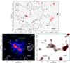 |
Fig. 1 Z5247: Top: GMRT 610 MHz high resolution image in contours (red +ve and cyan −ve) overlaid on SDSS r-band image in grey-scale. The contours are at −0.09,0.09,0.18,0.36,0.72,1.44,2.88,5.76 mJy beam-1. The beam at 610 MHz is 6.2′′ × 5.2′′, p.a. 56°. The discrete radio sources in the cluster region (A to I), the relic and the two BCGs (1 and 2) are labelled. The extent of the X-ray emission from the cluster ICM is shown by the black contour. Bottom left: the Chandra X-ray image (Obs ID 11727, 0.5−2 keV and resolution ~4′′) of Z5247 is shown in colour overlaid with the contours of the 60′′×60′′ resolution 610 MHz image (black +ve and cyan −ve) made after the subtraction of the discrete sources. The contours are at −0.9,0.9,1,1.2,1.8,2.4,3,4 mJy beam-1. The features in the X-rays are labelled in green (P1, P2 and NW Extension) and the positions of the BCGs (“×”) and of the discrete radio sources (“+”) are marked. Bottom right: the 60′′ × 60′′ resolution 610 MHz image is shown in grey-scale with the same contours as in the left panel. |
4.1.2. RXJ2129.6+0005: a mini-halo
RXJ2129.6+0005 is a relaxed cluster with a BCG at the centre hosting a strong radio source (Fig. 2). The radio source is unresolved at the highest resolution in our GMRT 610 MHz observation and has a flux density of 48.9 mJy. This central source is surrounded by a low-brightness extended emission that can be classified as a mini-halo (Fig. 2). It has a flux density of ~8.0 mJy at 610 MHz and an extent of 225 kpc (~1′) in the east-west and 110 kpc (~30′′) in the north-south directions. The flux density of the mini-halo at 235 MHz is 21 mJy. The residual flux density in the NVSS image after subtracting the flux density of the discrete source from the FIRST image implies a flux density of 2.4 mJy for the mini-halo at 1400 MHz. The mini-halo has a spectral index of ~1.2 over the frequency range of 235−1400 MHz (Fig. 3).
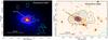 |
Fig. 2 RX J2129.6+0005: Left: GMRT 610 MHz low resolution image in contours (white +ve and cyan −ve) is overlaid on the Chandra X-ray image (Obs ID 09370, 0.5−2 keV and resolution ~2′′) in colour. The contours are at −0.11,0.33,0.44,0.55,0.66,0.88 mJy beam-1, and the beam is 11.6′′ × 10.6′′, p.a. 28°. The compact source at the centre marked by “×” has been subtracted. Right: the 610 MHz high resolution image in coutours (blue +ve and green −ve) is overlaid on the SDSS r-band image in colour. The contours are at −0.3,0.3,0.6,0.12,0.24,0.48 mJy beam-1, and the beam is 9.3′′ × 6.5′′, p.a. 48°. The central compact source S1 is identified with the BCG. The contours from the left panel are also shown (black and cyan). |
4.1.3. Z1953: a diffuse source
Z1953 (ZwCl 0847.2+3617) is a hot cluster classified as a merger based on optical and X-ray properties (Mann & Ebeling 2012). Three discrete radio sources (A, B, and C) are located in the central region of the cluster, aligned in the north-south direction (Fig. 4). To the west of these sources is a diffuse blob-like source, D. It has a roughly circular morphology with a diameter of ~210 kpc if assumed to be at the redshift of the Z1953. There is no obvious optical counterpart to D. It has a flux density of 5.2 mJy at 610 MHz. It is too small in size to be classified as a candidate radio halo ,and its position is offset from the central BCG, unlike typical mini-haloes. The dynamical activity in the cluster and its position make it an unusual mini-halo candidate. Thus we consider this to be unclassified diffuse emission.
4.1.4. A2552: a radio halo?
The cluster A2552 (RXC J2311.5+0338, MACS J2311.5+0338) is at a redshift of 0.305 (Ebeling et al. 2010). Four discrete sources are detected in the cluster’s central region at 610 MHz (Fig. 5, left): a is associated with the brightest cluster galaxy (BCG) in the cluster, and B and C have optical counterparts. The morphology of source D is reminiscent of a lobed radio galaxy; however, the lack of optical identification makes its classification uncertain. If assumed at the redshift of A2552, D has its largest linear extent of 180 kpc and a radio power of 2.6 × 1024 W Hz-1 at 610 MHz.
Patches of diffuse radio emission are detected in the cluster around the central source A (labelled H, Fig. 5, centre and right). The total flux density in the diffuse patches is ~10 mJy. However, a flux density of ~4.3 mJy is found in the image obtained after subtraction of the clean components of discrete sources. This is nearly at the level of the typical upper limits obtained in our work at 610 MHz. Although classified as a relaxed cluster based on the morphological parameter estimators, this cluster has been clssified as a “non cool-core” cluster based on X-ray and optical observations (Ebeling et al. 2010; Landry et al. 2013). We classify the diffuse emission in A2552 as a candidate radio halo. The sensitivity at 235 MHz is not sufficient to detect the emission. Deeper observations are needed to confirm it.
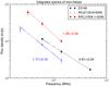 |
Fig. 3 Integrated spectra of the mini-haloes in RXJ2129.6+0005, Z3146 and RXCJ1504.1-0248 are plotted. The best fit lines and the inferred spectral indices of the mini-haloes are reported. The spectrum of RXCJ1504.1-0248 is scaled by a factor of 0.5 for visualisation in this plot. |
4.1.5. A3444 and S780
A 3444 and S 780 were observed in the first part of the survey and presented in V07. A 3444 was classified as a candidate mini-halo, while S 780 was considered as a non-detection, despite the hints of diffuse emission surrounding the central radio galaxy. More recently, Giacintucci et al. (in prep.) started a statistical investigation of the properties of mini-haloes and their host clusters, and revised all the GMRT non-detections and candidates, with analysis of archival VLA data at 1.4 GHz and of Chandra archival observations, not available at the time V07 was published. The good spatial coincidence of the X-ray features (cold front in S780 and an edge in A3444) with the radio morphology derived from the archival 1.4 GHz data and further imaging of the 610 MHz observations led to classifying both clusters as mini-haloes (Fig. 6). New images and the mini-halo properties will be discussed further in a future paper (Giacintucci et al., in prep.).
4.2. Non-detections and upper limits
The method of using injections to infer the detection limits on a radio halo flux density was introduced in the GRHS (V08, Brunetti et al. 2009) and is also continued to be used in the EGRHS (K13). A model radio halo of diameter 1 Mpc and a profile constructed from the profiles of observed radio haloes (Brunetti et al. 2007) is injected at the cluster centre in the final self-calibrated visibilities using the AIPS task “UVMOD”. The resulting visibilities are imaged and the detection of the radio halo is evaluated. Model radio haloes starting from high flux densities to gradually lower flux densities are injected until the detection in the image is similar to a marginal detection. The injected flux density corresponding to a “hint” of diffuse emission in them is considered as the upper limit for that particular data. The injections were carried out on 610 MHz data owing to their higher sensitivities.
The field of A68 is dominated by a double-lobed radio galaxy located at the southern edge of the cluster as seen in projection (Fig. 7, upper left). There is no optical identification for this radio galaxy, and thus it is likely a background source unrelated to the galaxy cluster. The cluster centre is affected by the residuals around the radio galaxy that are likely to bias an upper limit based on a central injection. An upper limit of 6 mJy was obtained with injections in a region offset from the cluster centre (~2′ towards west).
A1722 is a bright, relaxed cluster as inferred from the X-ray properties. However, the mass distribution is double peaked (Dahle et al. 2002). An upper limit of 3 mJy was obtained (Table 4). This is the deepest limit obtained amongst all the non-detections. To test whether a weak residual emission at the cluster centre was biasing our upper limit towards a lower value, we also made injections that are offset from the cluster centre (~5′). Similar upper limits were obtained in the offset injections, thus ruling out this bias.
Radio power upper limits using radio halo injections.
The cluster centres of RXCJ1212.3-1816 and A2485 (Fig. 7) are void of radio sources. In our earlier work (K13), upper limits based on 325 MHz data were presented for these clusters. Using the new 610 MHz data presented here, upper limits of 6 mJy and 5 mJy are estimated for these two clusters, respectively (Table 4). These are marginally deeper than those reported in K13.
Here we also point out an important caveat for interpreting the upper limits. They are obtained using a model radio halo of a given size and profile. The model is based on the profiles of a few well-known radio haloes, but there is a wide variety in the morphologies of the observed radio haloes as is also clear from the radio haloes in this survey (e.g. V07, V08, Brunetti et al. 2008). Therefore the upper limits are to be treated in the context of the specific model and not as generalised upper limits on the detection of diffuse emission with arbitrary or peculiar profiles.
In spite of such limitations, the upper limits are important outcomes of this survey, and they provide a tool for knowing where a cluster without a radio halo lies in the P1.4 GHz−LX plane relative to those with radio haloes. Limits have a statistical meaning and are useful in population studies. This method can be applied to any radio data to assess the detectability of a source of a particular morphology and brightness. The upcoming all-sky surveys with the next-generation instruments, such as the LOFAR and MWA, are expected to reach unprecedented surface brightness sensitivities and detect a large number of diffuse radio sources in galaxy clusters. The method used in EGRHS can be extended for use in these surveys to assess the non-detections.
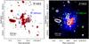 |
Fig. 4 Z1953: Left: GMRT 610 MHz image is shown in grey scale and in contours. The contours are at −0.15, 0.15, 0.2, 0.25, 0.3, 0.6, 1.2, 2.4, 4.8 mJy beam-1, and the beam is 9.3′′ × 6.5′′, p.a. 48°. The “+” marks the peak of the X-ray surface brightness. The discrete sources and the diffuse source are labelled. Right: the Chandra X-ray image (Obs ID 01659, 0.5−2 keV and resolution ~4′′) in colour overlaid with the 610 MHz contours from the left panel (white +ve and cyan −ve). |
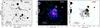 |
Fig. 5 A2552: Left: GMRT 610 MHz high resolution image in contours overlaid on the DSS POSS II R band image in grey scale. The contours are at −0.15,0.15,0.30,0.60,1.2 mJy beam-1, and the beam is 5.5′′ × 4.3′′, p.a. 35.9°. Middle: The 610 MHz low resolution (LR, 15′′ × 15′′) image in contours (white +ve and cyan −ve) overlaid on the Chandra X-ray image (Obs ID 11730, 0.5−2 keV and resolution ~4′′) in colour. The contours are at 0.4,0.6,0.8,1.6,3.2,6.4 mJy beam-1. The discrete sources are marked by “+”, and H points out the patches of diffuse emission. Right: the 610 MHz LR image in grey-scale and the contours same as in the middle panel (black +ve and cyan −ve) are overlaid. |
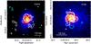 |
Fig. 6 A3444 and S780 Left: GMRT 610 MHz image of A3444 from V07 in contours (white +ve and cyan −ve) overlaid on the Chandra X-ray image (Obs ID 9400, 0.5−4 keV and resolution ~1′′) in colour. The contours are at 0.2 × ( ± 1,2,4,...) mJy beam-1, and the beam is 7.6′′ × 4.9′′, p.a. 19°. Right: GMRT 610 MHz image of S780 from the data presented in V07 shown in contours (white +ve and cyan −ve) overlaid on the Chandra X-ray image (Obs ID 9428, 0.5−4 keV and resolution of ~1′′) in colour. The contours are at 0.2 × ( ± 1,2,4,...) mJy beam-1, and the beam is 6′′ × 4′′. |
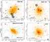 |
Fig. 7 GMRT 610 MHz images of A68, A1722, RXCJ1212.3-1816, and A2485 in contours (black +ve and cyan −ve) are shown overlaid on the respective Chandra X-ray images (colour). The contour levels are at 3σ × ( ± 1,2,4,8,...) in all the panels (see Table 2 for 1σ levels and the beam sizes). The 0.5−2 keV exposure-corrected Chandra X-ray images with resolution ~4′′ are presented for A68 (Obs ID 03250), A1722 (Obs ID 03278), and A2485 (Obs ID 10439) and an XMM-Newton (EPIC MOS) pipeline processed image (Observation number 0652010201, 0.2−12 keV, resolution ~8′′) for RXCJ1212.3-1816 is presented. |
4.3. RXCJ0510.7-0801
This cluster from the GRHS sample was observed at 610 and 235 MHz with the GMRT. The imaging of this cluster was affected by the presence of a strong radio source in the field of view. The rms noise achieved in the full resolution image at 610 MHz is 0.2 mJy beam-1 and at 235 MHz is 1.2 mJy beam-1 (Table 2). The images are presented in Fig. B.11. We have removed this cluster from the analysis because we lacked more sensitive images.
4.4. Imaging of known sources
4.4.1. Z3146
Z3146 (ZwCL 1021.0+0426) is a cool-core cluster in which a mini-halo was recently discovered using the 4.8 GHz VLA observations (Giacintucci et al. 2014b, hereafter, G14). We present the 610 MHz image of the cluster with the detection of the mini-halo. The compact source S1 is associated with the central galaxy (Fig. 8). The flux density of S2 is expected to be below 3σ, consistent with our lack of detection. The mini-halo surrounds the source S1 and its largest extent is 190 kpc detected at 610 MHz (Fig. 8). After subtracting the contribution from S1, the flux density of the mini-halo at 610 MHz is 11.5 mJy. This is consistent with the mini-halo spectral index ~1 over 1.4−4.8 GHz (G14) (Fig. 3). The different morphology of the mini-halo at 610 MHz and at 4.8 GHz (Fig. 8, centre) is due to the very different uv-coverage of the corresponding datasets, which span completely different hour angles.
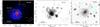 |
Fig. 8 Z3146: Left: GMRT 610 MHz image in contours (white +ve and cyan −ve) overlaid on the Chandra X-ray image (Obs ID 01651, 0.5−2 keV, resolution ~2′′) in colour. The contours are at 0.3 × (−1,1,2,4,...) mJy beam-1, and the beam is 8.9′′ × 7.1′′, p.a. 11.3°. Middle: The 4.8 GHz image from G14 is shown in grey scale overlaid with the 610 MHz contours from the left panel. Right: SDSS r-band image in colour showing the region near the BCG with the high resolution 610 MHz image overlaid in contours (black +ve and cyan −ve). The contours are at 0.3 × ( ± 1,2,4,...) mJy beam-1, and the beam is 5.8′′ × 3.9′′, p.a. 33.8°. |
4.4.2. RXCJ1504.1-0248
RXCJ1504.1-0248 is a cool-core cluster with a mini-halo detected at 327 MHz (GMRT) around its BCG (Giacintucci et al. 2011b, hereafter G11b). We present the 610 and 235 MHz images of the mini-halo (Figs. 9 and B.10). At 610 MHz the mini-halo has its largest linear extent of 290 kpc. At 325 MHz, the mini-halo is roughly circular (radius ~140 kpc) in morphology and shows a sharp fall in the surface brightness at the edges (G11b). The morphology is more extended and smoother at 610 MHz (Fig. 9). The spectral index of the mini-halo over the frequency range 235−140 MHz is estimated to be ~1.2 (Fig. 3).
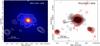 |
Fig. 9 RXC J1504.1-0248: Left: GMRT 610 MHz image in contours (white +ve and cyan −ve) overlaid on the Chandra X-ray image (Obs ID 05793, 0.5−2 keV, resolution ~2′′) in colour. The contours are at 0.4 × (−1,1,2,4,...) mJy beam-1, and the beam is 19.4′′ × 14.3′′, p.a. 70°. Right: the 610 MHz image is shown in grey scale with the 325 MHz image from G11b in contours (red +ve and cyan −ve). The 325 MHz contours are at 0.3 × ( ± 1,2,4,...) mJy beam-1, and the beam is 11.3′′ × 10.4′′. |
5. Analysis of the full GRHS and EGRHS sample
The combination of EGRHS and GRHS is at present the largest uniformly radio surveyed sample of galaxy clusters to search for diffuse emission. In the following, we refer to the GRHS and EGRHS as the full sample. The observations and the data analysis are complete, and the status of all the clusters in the full sample is reported (Table A.1). The GRHS and EGRHS sample (64) consists of all the clusters in the redshift range 0.2−0.4 that have X-ray luminosity, LX [0.1−2.4 keV]> 5 × 1044 erg s-1 with δ> −31°. The distribution of the full sample in X-ray luminosity and redshift is shown in Fig. 10.
We can summarise the findings of diffuse emission (see Table A.1, for references) in the full sample as follows:
-
Ten clusters have a radio halo (A209, A520, A697, A773, A1300,A1758a, A2163, A2219, RXCJ2003.5-2323,RXCJ1514.9-1523).
-
Two clusters host a radio halo and a relic (A2744, A521).
-
RXCJ1347.4-2515 has a radio halo and a double relic.
-
Nine clusters host a mini-halo (RXCJ1504.1-0248, A1835, Z3146, RXJ1532.9+3021, S780, A3444, A2390, RXJ2129.6+0005, Z7160).
Moreover, we found the following candidates:
-
Four candidate radio haloes (Z2661, A1682, Z5247, A2552).
-
Diffuse radio emission in Z1953, currently unclassified due to its size and location in the cluster.
-
Three candidate radio relics (A781, Z348, Z5247).
Upper limits on the flux density of a Mpc-sized radio halo were estimated for 30 clusters3. For three clusters with assessed absence of radio halo, we were unable to set an upper limit4. Owing to poor rms, no upper limits were derived for A 2813, A 2895, A 2645, A 963, and RXC J0510.7-0801. Finally, no information is available for RXCJ2211.7-0350. We removed these last six clusters from the statistical analysis ,so that our statistical analysis is based on a total of 58 clusters.
5.1. Fraction of radio haloes, mini-haloes, and radio relics
The fraction of radio haloes in the full sample is fRH = 13/58 = 22 ± 6% (here Poisson errors are used as a reference) and fRH = 17/58 = 29 ± 7% if the four candidate radio haloes are added. The fraction of mini-haloes is fMH = 9/58 = 16 ± 5%. These fractions are specific to the considered samples and will change if the cluster selection is made from a different parent catalogue.
The occurrence of radio haloes and mini-haloes as a function of X-ray luminosity and redshift is illustrated in the histograms (Fig. 11). It is striking from Figs. 10 and 11 (left) that the mini-haloes are detected in higher X-ray luminosity clusters in the sample, but the same is not the case with radio haloes. No statistically significant difference in the radio halo fraction in lower and higher luminosity bins was found in our sample. However, if the occurrence of radio haloes and mini-haloes is considered together, visual examination of Fig. 11 (left) indicates a higher occurrence for higher X-ray luminosity. We divided the sample into two bins using different values for the dividing X-ray luminosity and evaluated the occurrence of radio haloes and mini-haloes (RH+MH) in each bin. Using a Monte Carlo approach we found that the fraction, fRH + MH in the high X-ray luminosity bin differs with a 3.2σ significance from that in the low X-ray luminosity bin if the dividing X-ray luminosity is chosen to be 8 × 1044 erg s-1. In this case, the fRH + MH is 54% in the high X-ray luminosity bin and 10% in the low X-ray luminosity bin. The very high X-ray luminosity clusters are typically either strong cool cores or very hot merging clusters, and they can explain the high occurrence of a MH or a RH.
Our sample consists of X-ray luminous clusters selected from the flux-limited X-ray catalogues of clusters. It has been speculated that with this method, the relaxed, cool-core clusters are over represented, leading to a lower estimate of the occurrence of radio haloes than from a sample selected from a SZ selected cluster catalogue (Sommer & Basu 2014); see Cassano et al. (2013) for a first attempt to evaluate the occurrence of giant radio haloes in a mass-selected sub-sample of GRHS and EGRHS (extracted from the Planck SZ catalogue).
Radio relics occur as single or double arc-like sources at the peripheries of clusters. In the GRHS and EGRHS sample, double radio relics are known in RXCJ1314.4-2515, and single radio relics are known in A521 and A2744. Candidate radio relics are detected in A781, Z348, and Z5247. Thus, the fraction of radio relics is frelics = 3/58 = 5 ± 3%. If the candidate relics are also included, the fraction is 10 ± 4%.
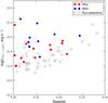 |
Fig. 10 GRHS and EGRHS sample in the X-ray luminosity − redshift plane. |
The overall occurrence of diffuse emission of any type (radio haloes, mini-haloes, and relics) in the 58 clusters is fdiff = 25/58 = 43 ± 9%. Thus, in general the occurrence of diffuse emission in clusters does not seem rare in massive and X-ray luminous galaxy clusters. The all-sky surveys with the next-generation instruments, such as the LOFAR and MWA with high sensitivity to low brightness emission are expected to reveal many more diffuse sources.
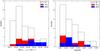 |
Fig. 11 Histograms showing the distribution of the GRHS and EGRHS sample in X-ray luminosity (left) and in redshift (right). The white histogram includes all the clusters (All), the red includes those with radio haloes (RHs), and the hatched includes those with mini-haloes (MHs). |
5.2. The P1.4GHz – LX diagram: haloes and mini-haloes
One of the main results from the GRHS was the bimodal distribution of the radio-loud and radio-quiet (absence of a giant radio halo) galaxy clusters found in the P1.4 GHz−LX plane. The distribution in the P1.4 GHz−LX plane of the clusters surveyed in the GRHS and EGRHS is presented in Fig. 12. The radio haloes in the literature listed in Cassano et al. (2013) are also plotted. The sensitivity of the survey has allowed a clear distinction between the clusters with giant radio haloes and those without. The ultra-steep spectrum (USS) are radio haloes with steep spectral indices (>1.5) that are all below the empirical P1.4 GHz−LX correlation. The radio halo in RXC J1314.4-2515 is the weakest of all the other radio haloes in clusters with similar X-ray luminosity (the black point immediately above the upper limits in Fig. 12). On one hand, we note that this is a giant radio halo, while on the other, it is possible that this source is still forming.
We also detected weak diffuse emission in two clusters, Z5247 and A2552 (candidate radio haloes, Sect. 4.1) that falls in the region occupied by the upper limits (stars). A linear fit using the BCES method (Akritas & Bershady 1996) of the form,  (1)was carried out for the radio haloes. We carried out separate fits by including and excluding the USS haloes in the data. The best fit parameters are: A = 2.13 ± 0.26 and B = −70.97 ± 11.52 (Fig. 12) and A = 2.24 ± 0.28 and B = −76.41 ± 12.65 (Fig. 12), excluding and including, respectively, the USS radio haloes from the data.
The distribution of clusters with mini-haloes in the P1.4 GHz−LX diagram is reported in Fig. 13, together with the upper limits for mini-halo detections in cool cores (K13). We found a possible trend between P1.4 GHz and the cluster X-ray luminosity. We fit this relation with Eq. (1), obtaining the best-fit parameters: A = 2.49 ± 0.30, B = −88.74 ± 13.92 (Fig. 13) and A = 3.37 ± 0.70, B = −128.60 ± 32.07, by using the bisector and orthogonal methods, respectively. There is a large scatter in the distribution, and the two methods lead to different slopes for the scaling. The upper limits obtained for the mini- (K13) are conservative and are not sufficient for testing whether there is bimodality. There are two main reasons for the conservative upper limits. The central bright radio source poses difficulties in obtaining deeper upper limits. Injections offset from the centre will be deeper, but will not represent the real mini-haloes that are found superposed on the central radio sources. In addition, the model radio halo profile scaled to the size of 500 kpc was used as a model for mini-halo injection (K13). The observed profiles of mini-haloes are more centrally peaked than for the radio haloes (Murgia et al. 2009) and can lead to slightly upper limits.
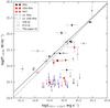 |
Fig. 12 Radio haloes and the upper limits (UL) in the GRHS and EGRHS sample are shown in the P1.4 GHz−LX diagram, along with the literature radio haloes listed in Cassano et al. (2013). The filled symbols are for radio haloes that belong to the GRHS and EGRHS sample, and the empty symbols are for the literature radio haloes. The squares are the USS radio haloes. The arrows show the upper limits from the current (red) and previous works (grey, V08 and blue, K13). The best fit lines to the radio haloes excluding the USS radio haloes (solid) and including the USS radio haloes (dashed) are also plotted. |
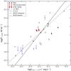 |
Fig. 13 Mini-haloes (filled symbols) and the upper limits (UL) from the GRHS and EGRHS are shown in the P1.4 GHz−LX diagram along with the literature mini-haloes (empty symbols). The best-fit lines using the BCES bisector (dashed) and orthogonal (solid) methods are also plotted. |
5.3. Cluster dynamics in GRHS and EGRHS
The non-thermal emission detected in the forms of radio haloes, relics, and mini-haloes are linked to the various forms of disturbances in the ICM. There is strong observational evidence to support the hypothesis that dynamical disturbance in clusters is closely connected to the generation mechanism of radio haloes (e.g. Cassano et al. 2010). Radio relics at cluster outskirts are tracers of shocks in cluster mergers. In the case of mini-haloes, the turbulence injected by the sloshing cool core may play a role (e.g. Gitti et al. 2006; Giacintucci et al. 2014b; ZuHone et al. 2013). The connection between the dynamical state and the diffuse emission can be closely examined using a large sample like GRHS and EGRHS.
The X-ray surface brightness maps represent the state of the thermal ICM, which is collisional and thus reveals the dynamical state of a cluster. The disturbance in the ICM can be quantified using the morphological state estimators on the X-ray surface brightness maps (e.g. Cassano et al. 2010). We used the cluster morphological state estimators described in (Cassano et al. 2010): the concentration parameter (c100), the centroid shift (w500 pe), and the power ratios (P3/P0cen) available for the GRHS and EGRHS clusters (Cassano et al. 2010, 2013; Cuciti et al., in prep.). The sample clusters are shown in the planes formed by these parameters with the markers distinguishing the clusters with radio haloes, mini-haloes, and with no radio emission (Fig. 14). While the clusters with mini-haloes and radio haloes appear well separated into quadrants for less and more disturbed clusters, the clusters that do not have any radio emission populate the region of both mini-haloes and radio haloes (Fig. 14).
That several merging clusters do not host a radio halo provides crucial information for the origin of these sources. If turbulence plays a role in the acceleration and dynamics of relativistic particles radio haloes evolve on a time scale of about 1 Gyr. According to this scenario, the possibility of generating a halo that is sufficiently luminous (detectable by our observations) at the GMRT frequencies depends on the combination of several parameters, including the magnetic field properties of the hosting cluster, the mass of the merging systems, the fraction of the energy of mergers that is drained in turbulence (and its properties), and the stage of the merger (Cassano et al. 2010; Russell et al. 2011; Donnert et al. 2013; Brunetti & Jones 2014, for a review). Further statistical studies that also consider information on the mass of clusters will be very useful. Interestingly, those merging clusters that do not show haloes at the level of current upper limits are also candidates for hosting ultra-steep-spectrum haloes that should be visible at lower frequencies (Brunetti et al. 2008; Cassano 2010); in this respect, future LOFAR observations will be particularly useful.
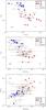 |
Fig. 14 GRHS and EGRHS clusters are shown in the planes formed by the morphological parameters, namely, the concentration parameter (c100), the centroid shift (w500pe), and the power ratio (P3/P0). The clusters that are non-detections (empty circles), those with radio haloes (red filled circles), those with mini-haloes (blue squares), and those with candidate radio haloes (A1682, Z5247, A2552, and Z2661; red stars) are marked. The grey dashed lines mark the boundaries proposed by Cassano et al. (2010) between the merging and the relaxed clusters for each of the parameters. |
6. Summary and conclusions
The GRHS and EGRHS together are a sample of 64 bright galaxy clusters surveyed at low frequency bands (610/235 MHz) to understand the statistical properties of diffuse radio emission in galaxy clusters. The sample consisted of all the galaxy clusters in the redshift range 0.2−0.4 that have X-ray luminosities, LX [0.1−2.4 keV]> 5 × 1044 erg s-1, and are above the declination of −31° selected from the REFLEX and the eBCS catalogues. This selection was tailored to suit the sensitivity of the GMRT at 610 MHz and also matched the redshift in which most of the radio haloes are expected to occur based on the turbulent reacceleration models. The results from the GRHS, based on the radio information on 35 clusters, were presented (V07, V08), after which the extension of the sample, called the EGRHS was carried out. The first part of the EGRHS data were presented in K13. In this work we have presented the final batch of 11 galaxy clusters and the statistical results based on the full sample.
Radio images of 11 galaxy clusters at 610 and 235 MHz with rms noise in the ranges 0.03−0.2 mJy beam-1 and 0.5−1.2 mJy beam-1, respectively, were presented and discussed. We discovered a mini-halo in the cluster RXC J2129.6+0005, a relic and a candidate radio halo in Z5247, a candidate radio halo in A2552, and an unclassified diffuse source in Z1953. The detections of mini-haloes in the GRHS clusters S780 and A3444 were also reported. The 610 MHz images of the mini-haloes in Z3146 and RXC J1504.1-0248 were compared with those in literature. After combining the 610 and 235 MHz data with that available from the literature, the integrated spectra of the mini-haloes in the clusters Z3146, RXCJ1504.1-0248, and RXC J2129.6+0005 were presented. The spectral indices are in the range 0.9−1.3. The method of model radio halo injection was used on four clusters in this work.
On completing the presentation of radio data analysis for all the clusters, we carried out a statistical analysis of the full sample. The results are as follows:
-
1.
There are a total of 64 clusters in the sample of which 48 were partof the GRHS and 16 additional formed the EGRHS sample. Thosethat had insufficient radio data in GRHS (V07, V08) were alsoincluded for new dual frequency (610−235 MHz) GMRT observations with the EGRHS. The full sample can be found in Table. A.1.
-
2.
The primary aim of the survey was to search for radio haloes, though other forms of diffuse emission were recorded. There are 13 radio haloes in the sample; 5 were discovered in the GRHS and 8 were known from the literature. The fraction of radio haloes in the full sample is fRH ~ 22% (and ~29% including the candidates).
-
3.
There are nine mini-haloes in the sample of which new radio data on five mini-haloes were presented in this survey. The fraction of mini-haloes in the sample is fMH ~ 16%.
-
4.
The combined occurrence fraction of radio haloes and mini-haloes is ~54% in the clusters with higher X-ray luminosities (LX> 8 × 1044 erg s-1) as compared to that of ~10% in the lower X-ray luminosities. Based on Monte Carlo analysis, this drop is significant at 3.2σ level.
-
5.
The fraction of clusters with confirmed radio relics in our sample is frelics ~ 5%. If the candidate relics were included, the fraction is ~10%. The relics are thus found to be even rarer than the radio haloes in this sample.
-
6.
In the cases of non-detection of a radio halo, an upper limit was determined. A total of 31 upper limits for the detections of radio haloes with 1 Mpc size and of a model profile based on observed radio haloes were reported in this survey. The upper limits are a unique outcome of this survey and provide vital grounding to the occurrence fractions of radio haloes reported in this work.
-
7.
The P1.4 GHz−LX diagram for the radio haloes including all the available information on detections and upper limits from the survey was presented. The bimodality in the distribution of detections and upper limits is evident.
-
8.
The mini-haloes were also plotted in the P1.4 GHz−LX diagram, along with the upper limits reported in K13. A bimodality is not seen in the distribution, though it cannot be ruled out. The mini-halo upper limits were based on a model radio-halo of size 500 kpc and thus are conservative.
-
9.
The morphological status estimators – the concentration parameter, centroid shift, and power ratios evaluated using the archival Chandra data for the survey clusters – were used as proxies for the dynamical state of the cluster. The regions occupied by the radio haloes and mini-haloes in the planes formed by these parameters are distinct; the radio haloes occur in merging clusters, whereas mini-haloes in relaxed clusters. The clusters with non-detections are found in both the merging and relaxed quadrants.
The completion of this survey provides the first uniformly surveyed sample on the occurrence of radio haloes. The methods for analysis presented in this survey can be applied in a broader context of future surveys with the next-generation telescopes, such as the JVLA, LOFAR, MWA, and eventually the SKA.
Online material
Appendix A: Online table
GRHS and EGRHS sample and results.
Appendix B: Radio images of the cluster fields
The radio images of the clusters up to the virial radius are presented here.
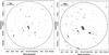 |
Fig. B.1 A68: GMRT 610 MHz (left) and 235 MHz (right) images in contours. Positive contours are black, and negative ones are grey in all the images in Appendix A. The contours are at 0.33 × ( ± 1,2,4,...) mJy beam-1 at 610 MHz and 6.0 × ( ± 1,2,4,...) mJy beam-1 at 235 MHz. The HPBWs at 610 and 235 MHz are 9.3′′ × 6.5′′, p.a. 47.9° and 29.0′′ × 12.7′′, p.a. 52.2°, respectively. The 1σ levels in the 610 and 235 MHz images are 0.05 and 1.5 mJy beam-1, respectively. The circle has a radius equal to the virial radius for this cluster (12.0′). |
 |
Fig. B.2 RXCJ1212.3-1816: GMRT 610 MHz image in contours. The contours are at 0.3 × ( ± 1,2,4,...) mJy beam-1. The HPBW at 610 is 11.4′′ × 5.7′′, p.a. 47.6°. The 1σ levels in the 610 MHz is 0.07 mJy beam-1. The circle has a radius equal to the virial radius for this cluster (10.4′). |
 |
Fig. B.3 A2485: GMRT 610 MHz (left) and 235 MHz (right) images in contours. The contours are at 0.18 × ( ± 1,2,4,...) mJy beam-1 at 610 MHz and 3.0 × ( ± 1,2,4,...) mJy beam-1 at 235 MHz. The HPBWs at 610 and 235 MHz are 8.1′′ × 7.0′′, p.a. 9.2° and 14.9′′ × 11.5′′, p.a. 50.3°, respectively. The 1σ levels in the 610 and 235 MHz images are 0.06 and 1.0 mJy beam-1, respectively. The circle has a radius equal to the virial radius for this cluster (10.7′). |
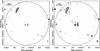 |
Fig. B.4 Z1953 (ZwCl0847.2+3617): GMRT 610 MHz (left) and 235 MHz (right) images in contours. The contours are at 0.45 × ( ± 1,2,4,...) mJy beam-1 at 610 MHz and 1.8 × ( ± 1,2,4,...) mJy beam-1 at 235 MHz. The HPBWs at 610 and 235 MHz are 7.2′′ × 6.9′′, p.a. −57.8° and 17.8′′ × 15.9′′, p.a. −14.7°, respectively. The 1σ levels in the 610 and 235 MHz images are 0.06 and 0.6 mJy beam-1, respectively. The circle has a radius equal to the virial radius for this cluster (10.6′). |
 |
Fig. B.5 Z5247 (RXC J1234.2+0947): GMRT 610 MHz (left) and 235 MHz (right) images in contours. The contours are at 0.09 × ( ± 1,2,4,...) mJy beam-1 at 610 MHz and 2.4 × ( ± 1,2,4,...) mJy beam-1 at 235 MHz. The HPBWs at 610 and 235 MHz are 6.2′′ × 5.2′′, p.a. 56° and 13.0′′ × 12.3′′, p.a. 71.4°, respectively. The 1σ levels in the 610 and 235 MHz images are 0.03 and 0.6 mJy beam-1, respectively. The circle has a radius equal to the virial radius for this cluster (10.6′). |
 |
Fig. B.6 A2552: GMRT 610 MHz (left) and 235 MHz (right) images in contours. The contours are at 0.21 × ( ± 1,2,4,...) mJy beam-1 at 610 MHz and 2.7 × ( ± 1,2,4,...) mJy beam-1 at 235 MHz. The HPBWs at 610 and 235 MHz are 9.2′′ × 7.2′′, p.a. 50.4° and 16.2′′ × 13.4′′, p.a. 9.6°, respectively. The 1σ levels in the 610 and 235 MHz images are 0.07 and 0.7 mJy beam-1, respectively. The circle has a radius equal to the virial radius for this cluster (10.5′). |
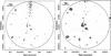 |
Fig. B.7 Z3146 (ZwCL1021.0+0426): GMRT 610 MHz (left) and 235 MHz (right) images in contours. The contours are at 0.6 × ( ± 1,2,4,...) mJy beam-1 at 610 MHz and 3.3 × ( ± 1,2,4,...) mJy beam-1 at 235 MHz. The HPBWs at 610 and 235 MHz are 8.9′′ × 7.1′′, p.a. 11.3° and 26.7′′ × 21.1′′, p.a. 47.8°, respectively. The 1σ levels in the 610 and 235 MHz images are 0.09 and 1.1 mJy beam-1, respectively. The circle has a radius equal to the virial radius for this cluster (12.2′). |
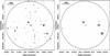 |
Fig. B.8 A1722: GMRT 610 MHz (left) and 235 MHz (right) images in contours. The contours are at 0.18 × ( ± 1,2,4,...) mJy beam-1 at 610 MHz and 5.0 × ( ± 1,2,4,...) mJy beam-1 at 235 MHz. The HPBWs at 610 and 235 MHz are 8.4′′ × 7.3′′, p.a. −9.9° and 26.2′′ × 24.3′′, p.a. −48.6°, respectively. The 1σ levels in the 610 and 235 MHz images are 0.04 and 0.9 mJy beam-1, respectively. The circle has a radius equal to the virial radius for this cluster (9.9′). |
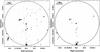 |
Fig. B.9 RX J2129.6+0005: GMRT 610 MHz (left) and 235 MHz (right) images in contours. The contours are at 0.3 × ( ± 1,2,4,...) mJy beam-1 at 610 MHz and 6.0 × ( ± 1,2,4,...) mJy beam-1 at 235 MHz. The HPBWs at 610 and 235 MHz are 7.9′′ × 6.3′′, p.a. 29.3° and 14.5′′ × 11.3′′, p.a. 53.8°, respectively. The 1σ levels in the 610 and 235 MHz images are 0.08 and 0.9 mJy beam-1, respectively. The circle has a radius equal to the virial radius for this cluster (13.5′). |
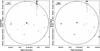 |
Fig. B.10 RXC J1504.1-0248: GMRT 610 MHz (left) and 235 MHz (right) images in contours. The contours are at 1.0 × ( ± 1,2,4,...) mJy beam-1 at 610 MHz and 6.0 × ( ± 1,2,4,...) mJy beam-1 at 235 MHz. The HPBWs at 610 and 235 MHz are 7.9′′ × 6.3′′, p.a. 29.3° and 14.5′′ × 11.3′′, p.a. 53.8°, respectively. The 1σ levels in the 610 and 235 MHz images are 0.08 and 0.9 mJy beam-1, respectively. The circle has a radius equal to the virial radius for this cluster (17.8′). |
 |
Fig. B.11 RXC J0510.7-0801: GMRT 610 MHz (left) and 235 MHz (right) images in contours. The contours are at 0.8 × ( ± 1,2,4,...) mJy beam-1 at 610 MHz and 6.0 × ( ± 1,2,4,...) mJy beam-1 at 235 MHz. The HPBWs at 610 and 235 MHz are 5.4′′ × 4.8′′, p.a. 41.1° and 15.7′′ × ′′13.1, p.a. 69.6°, respectively. The 1σ levels in the 610 and 235 MHz images are 0.2 and 1.2 mJy beam-1, respectively. The circle has a radius equal to the virial radius for this cluster (13.3′). |
We remove the clusters RXC J1512.2-2254, Abell 689, and RXJ2228.6+2037 from the combined sample of 67 clusters reported until K13. The REFLEX catalogue source RXC J1512.2-2254 in the GRHS sample (V07, V08) contains no spectroscopically confirmed member galaxies (Guzzo et al. 2009). The X-ray luminosity of the cluster Abell 689 after subtracting the central point source reported in Giles et al. (2012) pushes it below our lower luminosity limit for selection. The redshift of RXJ2228.6+2037 is above the survey cut-off of 0.4.
Acknowledgments
We thank the staff of the GMRT, who have made these observations possible. GMRT is run by the National Centre for Radio Astrophysics of the Tata Institute of Fundamental Research. The National Radio Astronomy Observatory is a facility of the National Science Foundation operated under cooperative agreement by Associated Universities, Inc. This research made use of the NASA/IPAC Extragalactic Database (NED), which is operated by the Jet Propulsion Laboratory, California Institute of Technology, under contract with the National Aeronautics and Space Administration. We made use of the ROSAT Data Archive of the Max-Planck-Institut fur extraterrestrische Physik (MPE) at Garching, Germany. This research made use of data obtained from the High Energy Astrophysics Science Archive Research Center (HEASARC), provided by NASA’s Goddard Space Flight Center. This work is partially supported by PRIN-INAF2008 and by FP-7-PEOPLE-2009-IRSES CAFEGroups project grant agreement 247653. GM acknowledges financial support by the “Agence Nationale de la Recherche” through grant ANR-09-JCJC-0001-01. R.K. thanks J. Donnert for insightful discussions.
References
- Akritas, M. G., & Bershady, M. A. 1996, ApJ, 470, 706 [NASA ADS] [CrossRef] [Google Scholar]
- Baars, J. W. M., Genzel, R., Pauliny-Toth, I. I. K., & Witzel, A. 1977, A&A, 61, 99 [NASA ADS] [Google Scholar]
- Basu, K. 2012, MNRAS, 421, L112 [NASA ADS] [CrossRef] [Google Scholar]
- Blasi, P., & Colafrancesco, S. 1999, Astropart. Phys., 12, 169 [NASA ADS] [CrossRef] [Google Scholar]
- Böhringer, H., Schuecker, P., Guzzo, L., et al. 2004, A&A, 425, 367 [NASA ADS] [CrossRef] [EDP Sciences] [Google Scholar]
- Bonafede, A., Intema, H. T., Brüggen, M., et al. 2014, MNRAS, 444, L44 [NASA ADS] [CrossRef] [Google Scholar]
- Brunetti, G., & Jones, T. W. 2014, Int. J. Mod. Phys. D, 23, 30007 [Google Scholar]
- Brunetti, G., & Lazarian, A. 2011, MNRAS, 410, 127 [NASA ADS] [CrossRef] [Google Scholar]
- Brunetti, G., Setti, G., Feretti, L., & Giovannini, G. 2001, MNRAS, 320, 365 [NASA ADS] [CrossRef] [Google Scholar]
- Brunetti, G., Venturi, T., Dallacasa, D., et al. 2007, ApJ, 670, L5 [NASA ADS] [CrossRef] [Google Scholar]
- Brunetti, G., Giacintucci, S., Cassano, R., et al. 2008, Nature, 455, 944 [NASA ADS] [CrossRef] [Google Scholar]
- Brunetti, G., Cassano, R., Dolag, K., & Setti, G. 2009, A&A, 507, 661 [NASA ADS] [CrossRef] [EDP Sciences] [Google Scholar]
- Cassano, R. 2010, A&A, 517, A10 [NASA ADS] [CrossRef] [EDP Sciences] [Google Scholar]
- Cassano, R., Brunetti, G., & Setti, G. 2006, MNRAS, 369, 1577 [NASA ADS] [CrossRef] [Google Scholar]
- Cassano, R., Ettori, S., Giacintucci, S., et al. 2010, ApJ, 721, L82 [NASA ADS] [CrossRef] [Google Scholar]
- Cassano, R., Ettori, S., Brunetti, G., et al. 2013, ApJ, 777, 141 [NASA ADS] [CrossRef] [Google Scholar]
- Chandra, P., Ray, A., & Bhatnagar, S. 2004, ApJ, 612, 974 [NASA ADS] [CrossRef] [Google Scholar]
- Crawford, C. S., Allen, S. W., Ebeling, H., Edge, A. C., & Fabian, A. C. 1999, MNRAS, 306, 857 [NASA ADS] [CrossRef] [Google Scholar]
- Dahle, H., Kaiser, N., Irgens, R. J., Lilje, P. B., & Maddox, S. J. 2002, ApJS, 139, 313 [NASA ADS] [CrossRef] [Google Scholar]
- Dennison, B. 1980, ApJ, 239, L93 [NASA ADS] [CrossRef] [Google Scholar]
- Dolag, K., & Enßlin, T. A. 2000, A&A, 362, 151 [NASA ADS] [Google Scholar]
- Donnert, J., Dolag, K., Brunetti, G., & Cassano, R. 2013, MNRAS, 429, 3564 [NASA ADS] [CrossRef] [Google Scholar]
- Ebeling, H., Edge, A. C., Bohringer, H., et al. 1998, MNRAS, 301, 881 [NASA ADS] [CrossRef] [Google Scholar]
- Ebeling, H., Edge, A. C., Allen, S. W., et al. 2000, MNRAS, 318, 333 [NASA ADS] [CrossRef] [Google Scholar]
- Ebeling, H., Edge, A. C., Mantz, A., et al. 2010, MNRAS, 407, 83 [NASA ADS] [CrossRef] [Google Scholar]
- Feretti, L., Giovannini, G., Govoni, F., & Murgia, M. 2012, A&ARv, 20, 54 [Google Scholar]
- Fujita, Y., Matsumoto, T., & Wada, K. 2004, J. Kor. Astron. Soc., 37, 571 [Google Scholar]
- Giacintucci, S., Venturi, T., Macario, G., et al. 2008, A&A, 486, 347 [NASA ADS] [CrossRef] [EDP Sciences] [Google Scholar]
- Giacintucci, S., Dallacasa, D., Venturi, T., et al. 2011a, A&A, 534, A57 [NASA ADS] [CrossRef] [EDP Sciences] [Google Scholar]
- Giacintucci, S., Markevitch, M., Brunetti, G., Cassano, R., & Venturi, T. 2011b, A&A, 525, L10 [NASA ADS] [CrossRef] [EDP Sciences] [Google Scholar]
- Giacintucci, S., Markevitch, M., Brunetti, G., et al. 2014a, ApJ, 795, 73 [NASA ADS] [CrossRef] [Google Scholar]
- Giacintucci, S., Markevitch, M., Venturi, T., et al. 2014b, ApJ, 781, 9 [NASA ADS] [CrossRef] [Google Scholar]
- Giles, P. A., Maughan, B. J., Birkinshaw, M., Worrall, D. M., & Lancaster, K. 2012, MNRAS, 419, 503 [NASA ADS] [CrossRef] [Google Scholar]
- Giovannini, G., Tordi, M., & Feretti, L. 1999, New Astron., Rev., 4, 141 [Google Scholar]
- Gitti, M., Feretti, L., & Schindler, S. 2006, A&A, 448, 853 [NASA ADS] [CrossRef] [EDP Sciences] [Google Scholar]
- Guo, X., Sironi, L., & Narayan, R. 2014, ApJ, 797, 47 [NASA ADS] [CrossRef] [Google Scholar]
- Guzzo, L., Schuecker, P., Böhringer, H., et al. 2009, A&A, 499, 357 [NASA ADS] [CrossRef] [EDP Sciences] [Google Scholar]
- Haslam, C. G. T., Kronberg, P. P., Waldthausen, H., Wielebinski, R., & Schallwich, D. 1978, A&AS, 31, 99 [NASA ADS] [Google Scholar]
- Jaffe, W. J., & Rudnick, L. 1979, ApJ, 233, 453 [NASA ADS] [CrossRef] [Google Scholar]
- Kale, R., Dwarakanath, K. S., Bagchi, J., & Paul, S. 2012, MNRAS, 426, 1204 [NASA ADS] [CrossRef] [Google Scholar]
- Kale, R., Venturi, T., Giacintucci, S., et al. 2013, A&A, 557, A99 [NASA ADS] [CrossRef] [EDP Sciences] [Google Scholar]
- Kang, H., & Ryu, D. 2011, ApJ, 734, 18 [NASA ADS] [CrossRef] [Google Scholar]
- Kang, H., Ryu, D., & Jones, T. W. 2012, ApJ, 756, 97 [Google Scholar]
- Keshet, U., & Loeb, A. 2010, ApJ, 722, 737 [NASA ADS] [CrossRef] [Google Scholar]
- Landry, D., Bonamente, M., Giles, P., et al. 2013, MNRAS, 433, 2790 [NASA ADS] [CrossRef] [Google Scholar]
- Liang, H., Hunstead, R. W., Birkinshaw, M., & Andreani, P. 2000, ApJ, 544, 686 [NASA ADS] [CrossRef] [Google Scholar]
- Mann, A. W., & Ebeling, H. 2012, MNRAS, 420, 2120 [NASA ADS] [CrossRef] [Google Scholar]
- Markevitch, M., Govoni, F., Brunetti, G., & Jerius, D. 2005, ApJ, 627, 733 [NASA ADS] [CrossRef] [Google Scholar]
- Mazzotta, P., & Giacintucci, S. 2008, ApJ, 675, L9 [NASA ADS] [CrossRef] [Google Scholar]
- Murgia, M., Govoni, F., Markevitch, M., et al. 2009, A&A, 499, 679 [NASA ADS] [CrossRef] [EDP Sciences] [Google Scholar]
- Petrosian, V. 2001, ApJ, 557, 560 [NASA ADS] [CrossRef] [Google Scholar]
- Petrosian, V., & East, W. E. 2008, ApJ, 682, 175 [NASA ADS] [CrossRef] [Google Scholar]
- Pfrommer, C., & Enßlin, T. A. 2004, A&A, 413, 17 [NASA ADS] [CrossRef] [EDP Sciences] [Google Scholar]
- Pinzke, A., Oh, S. P., & Pfrommer, C. 2013, MNRAS, 435, 1061 [NASA ADS] [CrossRef] [Google Scholar]
- Planck Collaboration XXIX. 2014, A&A, 571, A29 [NASA ADS] [CrossRef] [EDP Sciences] [Google Scholar]
- Russell, H. R., van Weeren, R. J., Edge, A. C., et al. 2011, MNRAS, 417, L1 [NASA ADS] [CrossRef] [Google Scholar]
- Russell, H. R., McNamara, B. R., Sanders, J. S., et al. 2012, MNRAS, 423, 236 [NASA ADS] [CrossRef] [Google Scholar]
- Ryu, D., Kang, H., Cho, J., & Das, S. 2008, Science, 320, 909 [NASA ADS] [CrossRef] [PubMed] [Google Scholar]
- Sommer, M. W., & Basu, K. 2014, MNRAS, 437, 2163 [NASA ADS] [CrossRef] [Google Scholar]
- Stroe, A., Harwood, J. J., Hardcastle, M. J., & Röttgering, H. J. A. 2014, MNRAS, 445, 1213 [NASA ADS] [CrossRef] [Google Scholar]
- Subramanian, K., Shukurov, A., & Haugen, N. E. L. 2006, MNRAS, 366, 1437 [NASA ADS] [CrossRef] [Google Scholar]
- van Weeren, R. J., Röttgering, H. J. A., Bagchi, J., et al. 2009, A&A, 506, 1083 [NASA ADS] [CrossRef] [EDP Sciences] [Google Scholar]
- van Weeren, R. J., Röttgering, H. J. A., Brüggen, M., & Hoeft, M. 2010, Science, 330, 347 [NASA ADS] [CrossRef] [PubMed] [Google Scholar]
- van Weeren, R. J., Röttgering, H. J. A., Intema, H. T., et al. 2012, A&A, 546, A124 [NASA ADS] [CrossRef] [EDP Sciences] [Google Scholar]
- Vazza, F., & Brüggen, M. 2014, MNRAS, 437, 2291 [NASA ADS] [CrossRef] [Google Scholar]
- Venturi, T., Giacintucci, S., Brunetti, G., et al. 2007, A&A, 463, 937 [NASA ADS] [CrossRef] [EDP Sciences] [Google Scholar]
- Venturi, T., Giacintucci, S., Dallacasa, D., et al. 2008, A&A, 484, 327 [NASA ADS] [CrossRef] [EDP Sciences] [Google Scholar]
- Vink, J., & Yamazaki, R. 2014, ApJ, 780, 125 [NASA ADS] [CrossRef] [Google Scholar]
- Zandanel, F., Pfrommer, C., & Prada, F. 2014, MNRAS, 438, 124 [NASA ADS] [CrossRef] [Google Scholar]
- ZuHone, J. A., Markevitch, M., Brunetti, G., & Giacintucci, S. 2013, ApJ, 762, 78 [NASA ADS] [CrossRef] [Google Scholar]
All Tables
All Figures
|
Fig. 1 Z5247: Top: GMRT 610 MHz high resolution image in contours (red +ve and cyan −ve) overlaid on SDSS r-band image in grey-scale. The contours are at −0.09,0.09,0.18,0.36,0.72,1.44,2.88,5.76 mJy beam-1. The beam at 610 MHz is 6.2′′ × 5.2′′, p.a. 56°. The discrete radio sources in the cluster region (A to I), the relic and the two BCGs (1 and 2) are labelled. The extent of the X-ray emission from the cluster ICM is shown by the black contour. Bottom left: the Chandra X-ray image (Obs ID 11727, 0.5−2 keV and resolution ~4′′) of Z5247 is shown in colour overlaid with the contours of the 60′′×60′′ resolution 610 MHz image (black +ve and cyan −ve) made after the subtraction of the discrete sources. The contours are at −0.9,0.9,1,1.2,1.8,2.4,3,4 mJy beam-1. The features in the X-rays are labelled in green (P1, P2 and NW Extension) and the positions of the BCGs (“×”) and of the discrete radio sources (“+”) are marked. Bottom right: the 60′′ × 60′′ resolution 610 MHz image is shown in grey-scale with the same contours as in the left panel. |
| In the text | |
|
Fig. 2 RX J2129.6+0005: Left: GMRT 610 MHz low resolution image in contours (white +ve and cyan −ve) is overlaid on the Chandra X-ray image (Obs ID 09370, 0.5−2 keV and resolution ~2′′) in colour. The contours are at −0.11,0.33,0.44,0.55,0.66,0.88 mJy beam-1, and the beam is 11.6′′ × 10.6′′, p.a. 28°. The compact source at the centre marked by “×” has been subtracted. Right: the 610 MHz high resolution image in coutours (blue +ve and green −ve) is overlaid on the SDSS r-band image in colour. The contours are at −0.3,0.3,0.6,0.12,0.24,0.48 mJy beam-1, and the beam is 9.3′′ × 6.5′′, p.a. 48°. The central compact source S1 is identified with the BCG. The contours from the left panel are also shown (black and cyan). |
| In the text | |
|
Fig. 3 Integrated spectra of the mini-haloes in RXJ2129.6+0005, Z3146 and RXCJ1504.1-0248 are plotted. The best fit lines and the inferred spectral indices of the mini-haloes are reported. The spectrum of RXCJ1504.1-0248 is scaled by a factor of 0.5 for visualisation in this plot. |
| In the text | |
|
Fig. 4 Z1953: Left: GMRT 610 MHz image is shown in grey scale and in contours. The contours are at −0.15, 0.15, 0.2, 0.25, 0.3, 0.6, 1.2, 2.4, 4.8 mJy beam-1, and the beam is 9.3′′ × 6.5′′, p.a. 48°. The “+” marks the peak of the X-ray surface brightness. The discrete sources and the diffuse source are labelled. Right: the Chandra X-ray image (Obs ID 01659, 0.5−2 keV and resolution ~4′′) in colour overlaid with the 610 MHz contours from the left panel (white +ve and cyan −ve). |
| In the text | |
|
Fig. 5 A2552: Left: GMRT 610 MHz high resolution image in contours overlaid on the DSS POSS II R band image in grey scale. The contours are at −0.15,0.15,0.30,0.60,1.2 mJy beam-1, and the beam is 5.5′′ × 4.3′′, p.a. 35.9°. Middle: The 610 MHz low resolution (LR, 15′′ × 15′′) image in contours (white +ve and cyan −ve) overlaid on the Chandra X-ray image (Obs ID 11730, 0.5−2 keV and resolution ~4′′) in colour. The contours are at 0.4,0.6,0.8,1.6,3.2,6.4 mJy beam-1. The discrete sources are marked by “+”, and H points out the patches of diffuse emission. Right: the 610 MHz LR image in grey-scale and the contours same as in the middle panel (black +ve and cyan −ve) are overlaid. |
| In the text | |
|
Fig. 6 A3444 and S780 Left: GMRT 610 MHz image of A3444 from V07 in contours (white +ve and cyan −ve) overlaid on the Chandra X-ray image (Obs ID 9400, 0.5−4 keV and resolution ~1′′) in colour. The contours are at 0.2 × ( ± 1,2,4,...) mJy beam-1, and the beam is 7.6′′ × 4.9′′, p.a. 19°. Right: GMRT 610 MHz image of S780 from the data presented in V07 shown in contours (white +ve and cyan −ve) overlaid on the Chandra X-ray image (Obs ID 9428, 0.5−4 keV and resolution of ~1′′) in colour. The contours are at 0.2 × ( ± 1,2,4,...) mJy beam-1, and the beam is 6′′ × 4′′. |
| In the text | |
|
Fig. 7 GMRT 610 MHz images of A68, A1722, RXCJ1212.3-1816, and A2485 in contours (black +ve and cyan −ve) are shown overlaid on the respective Chandra X-ray images (colour). The contour levels are at 3σ × ( ± 1,2,4,8,...) in all the panels (see Table 2 for 1σ levels and the beam sizes). The 0.5−2 keV exposure-corrected Chandra X-ray images with resolution ~4′′ are presented for A68 (Obs ID 03250), A1722 (Obs ID 03278), and A2485 (Obs ID 10439) and an XMM-Newton (EPIC MOS) pipeline processed image (Observation number 0652010201, 0.2−12 keV, resolution ~8′′) for RXCJ1212.3-1816 is presented. |
| In the text | |
|
Fig. 8 Z3146: Left: GMRT 610 MHz image in contours (white +ve and cyan −ve) overlaid on the Chandra X-ray image (Obs ID 01651, 0.5−2 keV, resolution ~2′′) in colour. The contours are at 0.3 × (−1,1,2,4,...) mJy beam-1, and the beam is 8.9′′ × 7.1′′, p.a. 11.3°. Middle: The 4.8 GHz image from G14 is shown in grey scale overlaid with the 610 MHz contours from the left panel. Right: SDSS r-band image in colour showing the region near the BCG with the high resolution 610 MHz image overlaid in contours (black +ve and cyan −ve). The contours are at 0.3 × ( ± 1,2,4,...) mJy beam-1, and the beam is 5.8′′ × 3.9′′, p.a. 33.8°. |
| In the text | |
|
Fig. 9 RXC J1504.1-0248: Left: GMRT 610 MHz image in contours (white +ve and cyan −ve) overlaid on the Chandra X-ray image (Obs ID 05793, 0.5−2 keV, resolution ~2′′) in colour. The contours are at 0.4 × (−1,1,2,4,...) mJy beam-1, and the beam is 19.4′′ × 14.3′′, p.a. 70°. Right: the 610 MHz image is shown in grey scale with the 325 MHz image from G11b in contours (red +ve and cyan −ve). The 325 MHz contours are at 0.3 × ( ± 1,2,4,...) mJy beam-1, and the beam is 11.3′′ × 10.4′′. |
| In the text | |
|
Fig. 10 GRHS and EGRHS sample in the X-ray luminosity − redshift plane. |
| In the text | |
|
Fig. 11 Histograms showing the distribution of the GRHS and EGRHS sample in X-ray luminosity (left) and in redshift (right). The white histogram includes all the clusters (All), the red includes those with radio haloes (RHs), and the hatched includes those with mini-haloes (MHs). |
| In the text | |
|
Fig. 12 Radio haloes and the upper limits (UL) in the GRHS and EGRHS sample are shown in the P1.4 GHz−LX diagram, along with the literature radio haloes listed in Cassano et al. (2013). The filled symbols are for radio haloes that belong to the GRHS and EGRHS sample, and the empty symbols are for the literature radio haloes. The squares are the USS radio haloes. The arrows show the upper limits from the current (red) and previous works (grey, V08 and blue, K13). The best fit lines to the radio haloes excluding the USS radio haloes (solid) and including the USS radio haloes (dashed) are also plotted. |
| In the text | |
|
Fig. 13 Mini-haloes (filled symbols) and the upper limits (UL) from the GRHS and EGRHS are shown in the P1.4 GHz−LX diagram along with the literature mini-haloes (empty symbols). The best-fit lines using the BCES bisector (dashed) and orthogonal (solid) methods are also plotted. |
| In the text | |
|
Fig. 14 GRHS and EGRHS clusters are shown in the planes formed by the morphological parameters, namely, the concentration parameter (c100), the centroid shift (w500pe), and the power ratio (P3/P0). The clusters that are non-detections (empty circles), those with radio haloes (red filled circles), those with mini-haloes (blue squares), and those with candidate radio haloes (A1682, Z5247, A2552, and Z2661; red stars) are marked. The grey dashed lines mark the boundaries proposed by Cassano et al. (2010) between the merging and the relaxed clusters for each of the parameters. |
| In the text | |
|
Fig. B.1 A68: GMRT 610 MHz (left) and 235 MHz (right) images in contours. Positive contours are black, and negative ones are grey in all the images in Appendix A. The contours are at 0.33 × ( ± 1,2,4,...) mJy beam-1 at 610 MHz and 6.0 × ( ± 1,2,4,...) mJy beam-1 at 235 MHz. The HPBWs at 610 and 235 MHz are 9.3′′ × 6.5′′, p.a. 47.9° and 29.0′′ × 12.7′′, p.a. 52.2°, respectively. The 1σ levels in the 610 and 235 MHz images are 0.05 and 1.5 mJy beam-1, respectively. The circle has a radius equal to the virial radius for this cluster (12.0′). |
| In the text | |
|
Fig. B.2 RXCJ1212.3-1816: GMRT 610 MHz image in contours. The contours are at 0.3 × ( ± 1,2,4,...) mJy beam-1. The HPBW at 610 is 11.4′′ × 5.7′′, p.a. 47.6°. The 1σ levels in the 610 MHz is 0.07 mJy beam-1. The circle has a radius equal to the virial radius for this cluster (10.4′). |
| In the text | |
|
Fig. B.3 A2485: GMRT 610 MHz (left) and 235 MHz (right) images in contours. The contours are at 0.18 × ( ± 1,2,4,...) mJy beam-1 at 610 MHz and 3.0 × ( ± 1,2,4,...) mJy beam-1 at 235 MHz. The HPBWs at 610 and 235 MHz are 8.1′′ × 7.0′′, p.a. 9.2° and 14.9′′ × 11.5′′, p.a. 50.3°, respectively. The 1σ levels in the 610 and 235 MHz images are 0.06 and 1.0 mJy beam-1, respectively. The circle has a radius equal to the virial radius for this cluster (10.7′). |
| In the text | |
|
Fig. B.4 Z1953 (ZwCl0847.2+3617): GMRT 610 MHz (left) and 235 MHz (right) images in contours. The contours are at 0.45 × ( ± 1,2,4,...) mJy beam-1 at 610 MHz and 1.8 × ( ± 1,2,4,...) mJy beam-1 at 235 MHz. The HPBWs at 610 and 235 MHz are 7.2′′ × 6.9′′, p.a. −57.8° and 17.8′′ × 15.9′′, p.a. −14.7°, respectively. The 1σ levels in the 610 and 235 MHz images are 0.06 and 0.6 mJy beam-1, respectively. The circle has a radius equal to the virial radius for this cluster (10.6′). |
| In the text | |
|
Fig. B.5 Z5247 (RXC J1234.2+0947): GMRT 610 MHz (left) and 235 MHz (right) images in contours. The contours are at 0.09 × ( ± 1,2,4,...) mJy beam-1 at 610 MHz and 2.4 × ( ± 1,2,4,...) mJy beam-1 at 235 MHz. The HPBWs at 610 and 235 MHz are 6.2′′ × 5.2′′, p.a. 56° and 13.0′′ × 12.3′′, p.a. 71.4°, respectively. The 1σ levels in the 610 and 235 MHz images are 0.03 and 0.6 mJy beam-1, respectively. The circle has a radius equal to the virial radius for this cluster (10.6′). |
| In the text | |
|
Fig. B.6 A2552: GMRT 610 MHz (left) and 235 MHz (right) images in contours. The contours are at 0.21 × ( ± 1,2,4,...) mJy beam-1 at 610 MHz and 2.7 × ( ± 1,2,4,...) mJy beam-1 at 235 MHz. The HPBWs at 610 and 235 MHz are 9.2′′ × 7.2′′, p.a. 50.4° and 16.2′′ × 13.4′′, p.a. 9.6°, respectively. The 1σ levels in the 610 and 235 MHz images are 0.07 and 0.7 mJy beam-1, respectively. The circle has a radius equal to the virial radius for this cluster (10.5′). |
| In the text | |
|
Fig. B.7 Z3146 (ZwCL1021.0+0426): GMRT 610 MHz (left) and 235 MHz (right) images in contours. The contours are at 0.6 × ( ± 1,2,4,...) mJy beam-1 at 610 MHz and 3.3 × ( ± 1,2,4,...) mJy beam-1 at 235 MHz. The HPBWs at 610 and 235 MHz are 8.9′′ × 7.1′′, p.a. 11.3° and 26.7′′ × 21.1′′, p.a. 47.8°, respectively. The 1σ levels in the 610 and 235 MHz images are 0.09 and 1.1 mJy beam-1, respectively. The circle has a radius equal to the virial radius for this cluster (12.2′). |
| In the text | |
|
Fig. B.8 A1722: GMRT 610 MHz (left) and 235 MHz (right) images in contours. The contours are at 0.18 × ( ± 1,2,4,...) mJy beam-1 at 610 MHz and 5.0 × ( ± 1,2,4,...) mJy beam-1 at 235 MHz. The HPBWs at 610 and 235 MHz are 8.4′′ × 7.3′′, p.a. −9.9° and 26.2′′ × 24.3′′, p.a. −48.6°, respectively. The 1σ levels in the 610 and 235 MHz images are 0.04 and 0.9 mJy beam-1, respectively. The circle has a radius equal to the virial radius for this cluster (9.9′). |
| In the text | |
|
Fig. B.9 RX J2129.6+0005: GMRT 610 MHz (left) and 235 MHz (right) images in contours. The contours are at 0.3 × ( ± 1,2,4,...) mJy beam-1 at 610 MHz and 6.0 × ( ± 1,2,4,...) mJy beam-1 at 235 MHz. The HPBWs at 610 and 235 MHz are 7.9′′ × 6.3′′, p.a. 29.3° and 14.5′′ × 11.3′′, p.a. 53.8°, respectively. The 1σ levels in the 610 and 235 MHz images are 0.08 and 0.9 mJy beam-1, respectively. The circle has a radius equal to the virial radius for this cluster (13.5′). |
| In the text | |
|
Fig. B.10 RXC J1504.1-0248: GMRT 610 MHz (left) and 235 MHz (right) images in contours. The contours are at 1.0 × ( ± 1,2,4,...) mJy beam-1 at 610 MHz and 6.0 × ( ± 1,2,4,...) mJy beam-1 at 235 MHz. The HPBWs at 610 and 235 MHz are 7.9′′ × 6.3′′, p.a. 29.3° and 14.5′′ × 11.3′′, p.a. 53.8°, respectively. The 1σ levels in the 610 and 235 MHz images are 0.08 and 0.9 mJy beam-1, respectively. The circle has a radius equal to the virial radius for this cluster (17.8′). |
| In the text | |
|
Fig. B.11 RXC J0510.7-0801: GMRT 610 MHz (left) and 235 MHz (right) images in contours. The contours are at 0.8 × ( ± 1,2,4,...) mJy beam-1 at 610 MHz and 6.0 × ( ± 1,2,4,...) mJy beam-1 at 235 MHz. The HPBWs at 610 and 235 MHz are 5.4′′ × 4.8′′, p.a. 41.1° and 15.7′′ × ′′13.1, p.a. 69.6°, respectively. The 1σ levels in the 610 and 235 MHz images are 0.2 and 1.2 mJy beam-1, respectively. The circle has a radius equal to the virial radius for this cluster (13.3′). |
| In the text | |
Current usage metrics show cumulative count of Article Views (full-text article views including HTML views, PDF and ePub downloads, according to the available data) and Abstracts Views on Vision4Press platform.
Data correspond to usage on the plateform after 2015. The current usage metrics is available 48-96 hours after online publication and is updated daily on week days.
Initial download of the metrics may take a while.