| Issue |
A&A
Volume 579, July 2015
|
|
|---|---|---|
| Article Number | A9 | |
| Number of page(s) | 22 | |
| Section | Extragalactic astronomy | |
| DOI | https://doi.org/10.1051/0004-6361/201425587 | |
| Published online | 19 June 2015 | |
Stellar hydrodynamical modeling of dwarf galaxies: simulation methodology, tests, and first results⋆
1
Department of AstrophysicsUniversity of Vienna,
Türkenschanzstrasse 17,
1180
Vienna,
Austria
e-mail:
This email address is being protected from spambots. You need JavaScript enabled to view it.
2
Research Institute of Physics, Southern Federal
University, Stachki
194, Rostov-on-Don,
Russia
Received: 25 December 2014
Accepted: 13 April 2015
Abstract
Context. In spite of enormous progress and brilliant achievements in cosmological simulations, they still lack numerical resolution or physical processes to simulate dwarf galaxies in sufficient detail. Accurate numerical simulations of individual dwarf galaxies are thus still in demand.
Aims. We aim to improve available numerical techniques to simulate individual dwarf galaxies. In particular, we aim to (i) study in detail the coupling between stars and gas in a galaxy, exploiting the so-called stellar hydrodynamical approach; and (ii) study for the first time the chemodynamical evolution of individual galaxies starting from self-consistently calculated initial gas distributions.
Methods. We present a novel chemodynamical code for studying the evolution of individual dwarf galaxies. In this code, the dynamics of gas is computed using the usual hydrodynamics equations, while the dynamics of stars is described by the stellar hydrodynamics approach, which solves for the first three moments of the collisionless Boltzmann equation. The feedback from stellar winds and dying stars is followed in detail. In particular, a novel and detailed approach has been developed to trace the aging of various stellar populations, which facilitates an accurate calculation of the stellar feedback depending on the stellar age. The code has been accurately benchmarked, allowing us to provide a recipe for improving the code performance on the Sedov test problem.
Results. We build initial equilibrium models of dwarf galaxies that take gas self-gravity into account and present different levels of rotational support. Models with high rotational support (and hence high degrees of flattening) develop prominent bipolar outflows; a newly-born stellar population in these models is preferentially concentrated to the galactic midplane. Models with little rotational support blow away a large fraction of the gas and the resulting stellar distribution is extended and diffuse. Models that start from non-self-gravitating initial equilibrium configurations, evolve at a much slower pace owing to lower initial gas density and hence lower star formation rates. The stellar dynamics turns out to be a crucial aspect of galaxy evolution. If we artificially suppress stellar dynamics, supernova explosions occur in a medium that is heated and diluted by previous activity of stellar winds, thus artificially enhancing stellar feedback.
Conclusions. The stellar hydrodynamics approach presents a promising tool for numerically studying the coupled evolution of gas and stars in dwarf galaxies.
Key words: Galaxy: abundances / galaxies: dwarf / Galaxy: evolution / galaxies: ISM / Galaxy: kinematics and dynamics
Appendices are available in electronic form at http://www.aanda.org
© ESO, 2015
1. Introduction
Cosmological simulations are currently reaching extraordinary levels of complexity and sophistication. Based on the so-called standard model of cosmology (SMoC), these state-of-the-art simulations are able to reproduce the main features of observed large galaxies (see, e.g., Brook et al. 2012; Zemp et al. 2012; Hopkins et al. 2013; Vogelsberger et al. 2014; Perret et al. 2014; Schaye et al. 2015), although severe disagreements with observations still persist (see, e.g., Genel et al. 2014). However, the resolution of these simulations still does not allow us to treat small-scale physics in dwarf galaxies (DGs).
Unfortunately, most of the weaknesses and problems shown by the SMoC manifest themselves in the range of masses typical for DGs (see, e.g., Kroupa 2012; Famaey & McGaugh 2012, 2013, for recent reviews). Besides full-blown cosmological simulations, it is thus necessary to run simulations of individual galaxies or small groups of galaxies. This enables us to study physical processes in greater numerical resolution and address the problems of the SMoC. The simulation of individual galaxies is therefore still extremely relevant. Also, very remarkable levels of accuracy have been reached in this field (see, e.g., Hopkins et al. 2013; Renaud et al. 2013; Roškar et al. 2013; Minchev et al. 2013; Teyssier et al. 2013, among others). The simulation of individual galaxies can also be used to parameterize feedback effects that can not be treated in cosmological simulations in detail (Creasey et al. 2013; Recchi 2014).
An obvious drawback of simulating individual galaxies is that it is not clear what initial conditions one should adopt. A common strategy is to consider a rotating, isothermal gas in equilibrium with the potential generated by a fixed distribution of stars and/or of dark matter (DM), but not with the potential generated by the gas itself (Tomisaka & Ikeuchi 1988; Silich & Tenorio-Tagle 1998; Mac-Low & Ferrara 1999; Recchi & Hensler 2013). A typical justification for neglecting gas self-gravity in DG simulations is that the mass budget of these objects should be dominated by DM. In our previous paper (Vorobyov et al. 2012), we explained in detail why this approach may produce unrealistic initial gas distributions and also considered the gas self-gravity when building equilibrium initial conditions.
As known from stellar structure studies (see, e.g., Ostriker & Mark 1968), the inclusion of gas self-gravity leads to implicit equations describing the initial equilibrium configuration, which must be solved iteratively. We did that for different halo masses, degrees of rotational support, and initial temperatures and we calculated the amount of gas prone to star formation for each of these models. Our star formation criteria were based on the Toomre instability criterium and on the Kennicutt-Schmidt empirical correlation between gas surface density and star formation rate (SFR) per unit area (see Vorobyov et al. 2012, for more details). For models that satisfy both star formation criteria, the underlying assumption was that the initial configuration is marginally stable to star formation and an external perturbing agent can trigger star formation in the corresponding parts of the galaxy.
The subsequent logical step is to use these marginally stable configurations as initial conditions for full-blown hydrodynamical simulations. For this purpose, we have developed a detailed 2+1 dimensional hydrodynamical code in cylindrical coordinates with assumed axial symmetry, which treats both the stellar and gaseous components as well as the phase transitions between them. Of course, a real galaxy may depart from such axial symmetry. However, since our initial conditions are axially symmetric and we do not explicitly consider environmental effects, the departures from axial symmetry are not expected to be significant.
This is the first of a series of papers devoted to numerically studying DGs with self-consistent initial conditions. Here, we explain in detail the basic strategy and the employed numerical hydrodynamical methods, which we extensively benchmark. Furthermore, we run a few representative models to show the overall early evolution of a typical DG. We pay particular attention to the co-evolution of stars and gas in our simulations. We follow the motion of stars by means of the so-called stellar hydrodynamical approach (Theis et al. 1992; Samland et al. 1997; Vorobyov & Theis 2006; Mitchell et al. 2013; Kulikov 2014), according to which the stellar component of a galaxy can be treated as a fluid. We develop this approach further and describe how stars and gas can be coupled by means of star formation and stellar feedback processes.
The paper is organized as follows. In Sect. 2 we describe the simulation methodology, paying specific attention to coupling the stars and gas via star formation and stellar feedback. Section 3 contains the gas cooling and heating rates employed in our modeling. The solution method of our stellar hydrodynamics equations is described in Sect. 4. The evolution of several representative models of DGs is studied in Sect. 5. Model caveats are discussed in Sect. 6. The main conclusions are summarized in Sect. 7, and we benchmark our code against a suite of test problems in the Appendix.
2. Simulation methodology
Our model DGs consist of a gas disk, a stellar component, and a fixed DM halo. The gas disk is a mixture of nine chemical elements (H, He, C, O, N, Ne, Mg, Si, and Fe), with the initial abundance of heavy elements set by the adopted initial metallicity. The stellar component consists of new stars born in the course of numerical simulations and has no pre-existing component. The DM halo has a spherically symmetric form and only contributes to the total gravitational potential of the system.
We describe the time evolution of our model galaxies using the coupled system of gas and stellar hydrodynamics equations complemented with phase transformations between stars and gas, chemical enrichment by supernova explosions, low- and intermediate-mass stars, as well as star formation feedback. We assume that individual chemical elements are dynamically well coupled with the bulk motion of the gas, which means that we only need to solve for the continuity equation for every chemical element with mass density ρi and do not need to solve for the dynamics of every element separately. Below, we provide a brief explanation for the key equations used to evolve our system in time.
2.1. Gas hydrodynamics
The dynamics of gas is modeled using the usual hydrodynamics equations for the gas density of ρg, momentum ρgvg, and internal energy density ϵ complemented with the rates of mass, momentum, and energy transfer between the gas and stellar components. The model also includes the continuity equations for the mass density of every chemical element ρi. The corresponding equations have the following form ![Mathematical equation: \begin{eqnarray} \label{contingas} &&{\partial \rho_{\rm g} \over \partial t} + \boldmath{\nabla} \cdot \left(\rho_{\rm g} \boldmath{v}_{\rm g} \right) = {\cal S} - {\cal D}, \\[2mm] &&{\partial \rho_{\rm i} \over \partial t} + \boldmath{\nabla} \cdot \left(\rho_{\rm i} \boldmath{v}_{\rm g} \right) = {\cal S}^{i} - {\cal D}^{i}, \\[2mm] \label{momgas} &&{\partial \over \partial t} \left (\rho_{\rm g} \boldmath{v}_{\rm g} \right) + \boldmath{\nabla } \cdot \left ( \rho_{\rm g} \boldmath{v}_{\rm g} \otimes \boldmath{v}_{\rm g} \right) = -\boldmath{\nabla} P +\rho_{\rm g} \boldmath{g}_{\rm gr} \nonumber \\ &&\hspace*{4cm}+ \boldmath{v}_{\rm s}{\cal S} - \boldmath{v}_{\rm g}{\cal D}, \\[2mm] \label{energy} &&{\partial \epsilon \over \partial t} + \boldmath{\nabla} \cdot \left( \epsilon \boldmath{v}_{\rm g} \right) = - P \boldmath{\nabla} \cdot \boldmath{v}_{\rm g} -\Lambda + \Gamma + \Gamma_\ast - \epsilon {{\cal D} \over \rho_{\rm g}}\cdot \end{eqnarray}](/articles/aa/full_html/2015/07/aa25587-14/aa25587-14-eq6.png) Here, vg and vs are the gas and stellar velocities, P = (γ − 1)ϵ is the gas pressure linked to the internal energy density via the ideal equation of state with the ratio of specific heats γ = 5/3, and ggr is the gravitational acceleration due to gas, stars, and DM halo. The gas cooling Λ due to line and continuum emission and gas heating Γ due to cosmic rays and small dust grains are explained in detail in Sect. 3. The gas heating due to stellar feedback Γ∗ is calculated as the sum of the contributions from SNII and SNIa explosions (ΓSNII and ΓSNIa, respectively), and also from the stellar winds Γsw. The last term on the r.h.s. of Eq. (4) accounts for the decrease in the internal energy due to formation of stars from the gas phase. We note that the quantity ρgvg ⊗ vg is the symmetric dyadic (a rank-two tensor) calculated according to the usual rules and ∇·(ρgvg⊗vg) is the divergence of a rank-two tensor.
Here, vg and vs are the gas and stellar velocities, P = (γ − 1)ϵ is the gas pressure linked to the internal energy density via the ideal equation of state with the ratio of specific heats γ = 5/3, and ggr is the gravitational acceleration due to gas, stars, and DM halo. The gas cooling Λ due to line and continuum emission and gas heating Γ due to cosmic rays and small dust grains are explained in detail in Sect. 3. The gas heating due to stellar feedback Γ∗ is calculated as the sum of the contributions from SNII and SNIa explosions (ΓSNII and ΓSNIa, respectively), and also from the stellar winds Γsw. The last term on the r.h.s. of Eq. (4) accounts for the decrease in the internal energy due to formation of stars from the gas phase. We note that the quantity ρgvg ⊗ vg is the symmetric dyadic (a rank-two tensor) calculated according to the usual rules and ∇·(ρgvg⊗vg) is the divergence of a rank-two tensor.
The source term  denotes the phase transformation of stars into the gas phase and is defined as the sum of the mass release rates (per unit volume) of all individual elements,
  . The mass release rate of a particular element i is defined as
  (5)where
  ,
,  , and
, and  are the contributions due to SNII, SNIa, and also due to low- and intermediate-mass stars, respectively. The sink term
  describes the phase transformation of gas into stars according to the adopted star formation law. The detailed explanation of all relevant rates is provided in Sect. 2.7.
2.2. Stellar hydrodynamics
The time evolution of the stellar component is computed using the Boltzmann moment equation approach introduced by Burkert & Hensler (1988), and is further developed in application to stellar disks in Samland et al. (1997) and Vorobyov & Theis (2006). In this approach, the dynamics of stars is described by the first three moments of the collisionless Boltzmann moment equations, ![Mathematical equation: \begin{eqnarray} \label{continstar} &&{\partial \rho_{\rm s} \over \partial t} + \boldmath{\nabla} \cdot \left(\rho_{\rm s} \boldmath{v}_{\rm s} \right) = {\cal D} - {\cal S}, \\[2mm] \label{momstar} &&{\partial \over \partial t} \left (\rho_{\rm s} \boldmath{v}_{\rm s} \right) + \boldmath{\nabla } \cdot \left (\boldmath{v}_{\rm s} \otimes \rho_{\rm s} \boldmath{v}_{\rm s} \right) = -\boldmath{\nabla} \cdot \boldmath{\Pi} +\rho_{\rm s} g_{\rm gr} - \boldmath{v}_{\rm s}{\cal S} + \boldmath{v}_{\rm g}{\cal D}, \quad\quad \\[2mm] \label{dispstar} &&{\partial \Pi_{ij} \over \partial t} + \boldmath{\nabla} \cdot \left( \Pi_{ij} \boldmath{v}_{\rm s} \right) = - \Pi_{ik}:(\boldmath{\nabla}\boldmath{v}_{\rm s})_{jk} - \Pi_{jk}:(\boldmath{\nabla}\boldmath{v}_{\rm s})_{ik} \nonumber \\[2mm] &&\hspace*{2.9cm} - \sigma_{ij}^2 {\cal S} + \sigma_{\ast}^2 {\cal D}, \end{eqnarray}](/articles/aa/full_html/2015/07/aa25587-14/aa25587-14-eq28.png) where ρs = m∫fd3u is the stellar mass density,
where ρs = m∫fd3u is the stellar mass density,  is the mean stellar velocity, and Π is the stress tensor with six components
  . The stellar velocity dispersions are defined as
  . The function f is the distribution function of stars in the six-dimensional, position-velocity phase space f ≡ f(t,x,u) and m is the average mass of a star. The quantity ∇vs is the gradient of a vector, the covariant expression for which is provided, e.g., in Stone & Norman (1992) and Πik: (∇vs)jk is the convolution (over index k) of two rank-two tensors. The quantity σ∗ represents a typical stellar velocity dispersion of a newborn cluster of stars, for which we take a fiducial value of 5.0 km s-1.
2.3. Massive stars
Massive stars that end their life with SNII explosions are main contributors to the energy budget and chemical composition of the interstellar medium. Therefore, it is important to follow their evolution as accurate as possible. We improve the description of the stellar component by solving for a separate continuity equation for the mass volume density  of stars with mass > 8.0 M⊙,
 (9)where fh is the fraction of stars with mass > 8.0 M⊙, calculated according to the adopted IMF (see Eq. (14)), and
  is the rate of death of massive stars. The massive star subcomponent has the same dynamical properties as the rest of the stars, an assumption that we plan to relax in the future.
2.4. Intermediate-mass stars
Stars in the (1.0−8.0) M⊙ mass range produce the majority of carbon and nitrogen. Moreover, binary stars in this mass range can explode as Type Ia supernovae and are thus important sources of iron. Therefore, we also solve for a separate continuity equation for the mass volume density  of intermediate-mass stars,
  (10)where fm is the fraction of stars with mass 1.0 M⊙<m< 8.0 M⊙ calculated according to the adopted IMF and
  is the rate of death of intermediate-mass stars. We note that the stellar evolution of low-mass stars can be neglected during the galactic evolution. They only contribute to the gravitational potential where their density can be deduced from ρs (the total stellar density),
  , and
, and  .
.
2.5. Gravity of gas, stars, and DM halo
The gravitational potential of gas and stars is calculated self-consistently by solving for the Poisson equation,  (11)To accelerate the simulations, we only solve for Eq. (11) when the relative error in the currently stored gravitational potential compared to the current density distribution exceeds 10-5 (see Stone & Norman 1992, for details).
The gravitational acceleration due to a spherically symmetric DM halo gh is calculated as explained in Vorobyov et al. (2012). Two options are available in the code: a cored isothermal DM halo profile and a Navarro-Frenk-White (or cuspy) profile. Here we use the cored isothermal DM profile. The total gravitational acceleration is calculated as ggr = gh − ∇Φg + s.
2.6. Mean stellar age
To calculate the mass and energy release rates by supernovae and dying low-mass stars one needs to know the age of stars. In the stellar hydrodynamics approach, stars are a mixture of populations with different ages. Nevertheless, one may define the mean age of stars  , which should obey the following rules:
-
1.
The bulk motion of stars, such as compression or rarefaction, should not affect the value of
. This can be achieved by solving for the Lagrangian or comoving equation for 
 (12)
(12) -
2.
A newly born stellar population should rejuvenate the pre-existing one. This is achieved by updating the mean age every time step in every grid cell, using the following equation:
 (13)where Ms is the stellar mass in a specific cell and △ Ms the mass of stars born in the same cell during time step △ t. Equation (13) satisfies the expected asymptotic behavior of the stellar age, which becomes small (
 ) during a massive instantaneous burst (△ Ms → ∞), but remains almost unchanged (
 ) in the quiescent phase △ Ms → 0.
 -
3.
The mean stellar age should uniformly increase with time, reflecting the overall aging of the system. This is done by adding the current time step △ t to the mean stellar age in every grid cell. Thus, in the absence of star formation and pre-existing old stellar population, the mean stellar age is equivalent to the current evolution time t.
In practice, we first solve for Eq. (12) to account for bulk motions, then we update the mean stellar age in every grid cell according to Eq. (13) to account for star formation, and finally we add the current time step △ t to the mean stellar age in every grid cell to take the aging of stellar populations into account. Since we follow the evolution of both the massive and intermediate-mass star subcomponents, their mean ages  and
and  , respectively, need to be calculated using the same procedure.
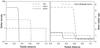 |
Fig. 1 Star volume density (left) and mean stellar age (right) as a function of time during the gravitational collapse of a stellar sphere of unit radius. The elapsed time is indicated in the left panel. Star formation is turned off for this test problem. The dash-dot-dotted lines shows the mean stellar age when calculated using the Eulerian form to account for bulk motions of stars instead of the Lagrangian form (see text for more detail). |
Figure 1 shows the time evolution of the stellar density ρs (left panel) and mean stellar age (right panel) in an idealized test problem involving the gravitational collapse of a stellar sphere with unit radius. Initially, ρs and are set to unity inside the sphere and to zero outside the sphere (dash-dotted lines). The stellar velocity dispersion is negligible everywhere and the SFR is set to zero. As the collapse proceeds, stellar density shows the expected behavior with a central plateau shrinking in size and growing in density. At the same time the mean stellar age increases in concordance with time, as expected in the absence of star formation. In particular, the difference between the values of inside and outside the sphere is always equal to unity, as was set initially. We emphasize here the need to use the Lagrangian equation for . If the Eulerian form 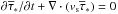 is used instead, the above test fails. Indeed, the dash-dot-dotted line shows the mean stellar age at t = 0.4 calculated using the Eulerian form. Evidently, the difference between the values of inside and outside the sphere is now much greater than unity, indicating a spurious aging of the stellar populations inside the sphere1.
Finally, we note that the concept of the mean stellar age has its limitations. For instance, in the case of a constant SFR and steady galaxy configuration, approaches a constant value after a few tens of Myr, meaning that the supernova rates and mass return rates (see Eqs. (17) and (19)) are exclusively determined by stars whose lifetime is equal to . This bias toward stars with single age (and mass) diminishes, when a time-varying SFR is present or stellar motions are taken into account. Nevertheless, a more sophisticated approach that takes into account a possible age spread around the mean value is desirable.
2.7. Source and sink terms
To calculate the rates at which stars return their mass (including newly synthesized elements) into the gas phase, we need to make assumptions about the initial mass function (IMF), stellar lifetimes, and nucleosynthesis rates.
We adopt the Kroupa IMF (Kroupa 2001) of the form, 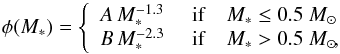 (14)where the normalization constants A and B are calculated as described in Sects. 2.7.1 and 2.7.2.
The stellar lifetimes are taken from Padovani & Matteucci (1993),  (15)where
  (16)In Eq. (15), we adjusted the transitional value for the stellar mass (7.45 M⊙) to obtain a smooth time derivative dM∗/ dτ.
2.7.1. Supernova type II rates
We assume that all stars in the ![Mathematical equation: \hbox{$[8.0~M_\odot\!\!: M_\ast^{\rm max}]$}](/articles/aa/full_html/2015/07/aa25587-14/aa25587-14-eq84.png) mass range end their life cycle as type II supernovae (SNeII), where
mass range end their life cycle as type II supernovae (SNeII), where  is the upper cut-off mass of the IMF set to 100 M⊙ in our model. The SNII rate, i.e., the number of SNeII per unit time, is then defined as
 ![Mathematical equation: \begin{equation} {\cal R}_{\rm SNII} = \left\{ \begin{array}{ll} \phi[M_\ast({\overline\tau}^{\rm h}_\ast)] { {\rm d}M_\ast({\overline\tau}^{\rm h}_\ast) \over {\rm d}\tau } \\[2mm] \hskip 1.2cm \mbox{if} \,\, \overline\tau^{h}_\ast\in [\tau(100~M_\odot)\!:\tau(8.0~M_\odot)], \\[1mm] 0 \hskip 1.cm \mbox{if} \,\, \overline\tau^{h}_\ast \ni [\tau(100~M_\odot)\!:\tau(8.0~M_\odot)], \end{array} \right. \label{SNII} \end{equation}](/articles/aa/full_html/2015/07/aa25587-14/aa25587-14-eq87.png) (17)where
(17)where  is the mass of a massive star that is about to die as SNII calculated by inverting Eq. (15). This is the SNII rate following an instantaneous burst of star formation. We therefore assume here that each star formation event generates a single stellar population (SSP). The superposition of SNII rates coming from many SSPs then approximates the SNII rate in the presence of a variable SFR. The derivative dM∗/ dτ is calculated by inverting Eq. (15) and then differentiating it with respect to time.
The IMF in Eq. (17) has to be normalized according to the total mass of massive stars  in each computational cell,
  (18)The upper limit in the integral is not fixed, rather it depends on the mean stellar age of massive stars in a given computational cell. This is done to take into account the fact that massive stars with lifetimes smaller than , and hence with mass greater than , must have exploded as SNeII. Excluding those stars ensures a correct calculation of the stellar mass spectrum at any time instant2. Since
  and are time-varying quantities, the normalization constants in the IMF need to be updated every time step.
The mass return rate (per unit volume) by SNII explosions can now be defined as ![Mathematical equation: \begin{equation} {\cal S}_{\rm SNII}^{i} = {\cal R}_{\rm SNII} \,\, \rho^i_{\rm SNII} \left[M_\ast(\overline\tau^{\rm h}_\ast)\right], \label{sourceSNII} \end{equation}](/articles/aa/full_html/2015/07/aa25587-14/aa25587-14-eq93.png) (19)where
(19)where ![Mathematical equation: \hbox{$\rho^i_{\rm SNII}[M_\ast(\overline\tau^{\rm h}_\ast)]$}](/articles/aa/full_html/2015/07/aa25587-14/aa25587-14-eq94.png) is the mass (per unit volume) released by a SNII of mass M∗ in the form of a specific element i. The values of ρi for nine considered elements (H, He, C, O, N, Ne, Mg, Si, and Fe) and four stellar metallicities (Z∗ = 10-4,10-2,10-1, and 1.0 times solar) are taken from Woosley & Weaver (1995). For stellar masses greater than 40 M⊙, the yields are set constant to those of a 40 M⊙ star.
is the mass (per unit volume) released by a SNII of mass M∗ in the form of a specific element i. The values of ρi for nine considered elements (H, He, C, O, N, Ne, Mg, Si, and Fe) and four stellar metallicities (Z∗ = 10-4,10-2,10-1, and 1.0 times solar) are taken from Woosley & Weaver (1995). For stellar masses greater than 40 M⊙, the yields are set constant to those of a 40 M⊙ star.
Finally, we assume that each supernova releases ϵSN × 1051 erg in the form of thermal energy and define the rate of energy density released by SNeII as  (20)where V is the injection volume specified by the actual size of our numerical grid and ϵSN is the ejection efficiency set to 1.0 in this work (see Sect. 6 for discussion).
2.7.2. Supernova type Ia rates
We derive the rates of Type Ia supernovae following the ideas and notations laid out in Matteucci & Recchi (2001). The number of binary systems (per unit mass of the binary system MB) that are capable of producing a SNIa explosion can be calculated as ![Mathematical equation: \begin{equation} N_{\rm SNIa}[M_2({\overline\tau}^{\rm m}_\ast)]= A_\ast \int \limits_{M_{\rm B,1}} \limits^{M_{\rm B,2}} \phi(M_{\rm B}) f\left( {M_2({\overline\tau}^{\rm m}_\ast) \over M_{\rm B}} \right) {{\rm d}M_{\rm B} \over M_{\rm B}}, \label{SNIa} \end{equation}](/articles/aa/full_html/2015/07/aa25587-14/aa25587-14-eq104.png) (21)where
(21)where  is the mass of the secondary component, A∗ a normalization constant and the limits of the integral are defined as
 ![Mathematical equation: \begin{eqnarray} M_{\rm B,1}&=&\max\left[2M_2({\overline\tau}^{\rm m}_\ast),M_{\rm B,min}\right] \\ M_{\rm B,2}&=&{1\over 2} M_{\rm B,max} + M_2({\overline\tau}^{\rm m}_\ast). \end{eqnarray}](/articles/aa/full_html/2015/07/aa25587-14/aa25587-14-eq107.png) The maximum and minimum masses of a binary system, which is capable of producing a SNIa explosion, are set to MB,min = 3.0 M⊙ and MB,max = 16.0 M⊙, respectively, and the maximum mass of the secondary is M2 = 8.0 M⊙. The quantity
The maximum and minimum masses of a binary system, which is capable of producing a SNIa explosion, are set to MB,min = 3.0 M⊙ and MB,max = 16.0 M⊙, respectively, and the maximum mass of the secondary is M2 = 8.0 M⊙. The quantity  in Eq. (21) is the distribution function of the
  ratio and is defined as
  (24)where γ is set to 0.5. For this value of γ, the normalization constant that better reproduces the observed [α/Fe] ratios in dwarf galaxies is A∗ = 0.06 (Recchi et al. 2009), therefore we adopt this value.
By analogy to the massive star subcomponent, the IMF in Eq. (21) has to be normalized according to the total mass of intermediate-mass stars  in each computational cell,
 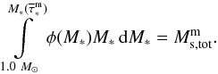 (25)The SNIa rate, i.e., the number of SNIa explosions per unit time, can now be calculated by analogy to Eq. (17) as
 ![Mathematical equation: \begin{equation} {\cal R}_{\rm SNIa} = \left\{ \begin{array}{ll} N_{\rm SNIa}\left[M_2({\overline\tau}^{\rm m}_\ast))\right] { {\rm d}M_2({\overline\tau}^{\rm m}_\ast)) \over {\rm d}\tau } \\ \hskip 1.2cm \mbox{if} \,\, {\overline\tau}^{\rm m}_\ast\in [\tau(8.0~M_\odot)\!\!:\tau(M_{\rm 2,min})], \\ 0 \hskip 1cm \mbox{if} \,\, {\overline\tau}^{\rm m}_\ast\ni [\tau(8.0~M_\odot)\!\!:\tau(M_{\rm 2,min})], \end{array} \right. \label{SNIaRate} \end{equation}](/articles/aa/full_html/2015/07/aa25587-14/aa25587-14-eq119.png) (26)where M2,min = 1.0M⊙ is the minimum mass of the secondary.
(26)where M2,min = 1.0M⊙ is the minimum mass of the secondary.
The mass return rate (per unit volume) by SNIa explosions can now be expressed as ![Mathematical equation: \begin{equation} {\cal S}_{\rm SNIa}^{i} = {\cal R}_{\rm SNIa} \, \rho^i_{\rm SNIa}[M_\ast({\overline\tau}^{\rm m}_\ast)], \label{sourceSNIa} \end{equation}](/articles/aa/full_html/2015/07/aa25587-14/aa25587-14-eq121.png) (27)where
(27)where ![Mathematical equation: \hbox{$\rho^i_{\rm SNIa}[M_\ast({\overline\tau}^{\rm m}_\ast)]$}](/articles/aa/full_html/2015/07/aa25587-14/aa25587-14-eq122.png) is the mass (per unit volume) released by a SNIa of mass M∗ in the form of a specific element i. The values of ρi for six elements (C, O, N, Mg, Si, and Fe) are taken from Nomoto et al. (1984). We neglect the metallicity dependence of the SNIa yields. The energy release rate by SNIa (ΓSNIa) is defined in analogy to Eq. (20), with ℛSNII being substituted by ℛSNIa.
is the mass (per unit volume) released by a SNIa of mass M∗ in the form of a specific element i. The values of ρi for six elements (C, O, N, Mg, Si, and Fe) are taken from Nomoto et al. (1984). We neglect the metallicity dependence of the SNIa yields. The energy release rate by SNIa (ΓSNIa) is defined in analogy to Eq. (20), with ℛSNII being substituted by ℛSNIa.
2.7.3. Stellar winds and the mass return by intermediate-mass stars
The luminosity produced by stellar winds is taken from results of the Starburst99 software package (Leitherer et al. 1999; Vazquez & Leitherer 2005). We used Padova AGB stellar tracks at different metallicities (Z∗ = 0.0004, 0.004, 0.008, 0.02, 0.05) and used this set of models as a library to obtain wind luminosities for each SSP, depending on its mass and average metallicity. The energy transfer efficiency of the wind power is set to 100%.
The mass-return rate (per unit volume) by winds of stars in the (1.0−8.0) M⊙ mass range is calculated as ![Mathematical equation: \begin{equation} {\cal S}^i_\ast={\cal R}_\ast \rho^i_\ast \left[M_\ast( {\overline\tau}^{\rm m}_\ast)\right], \end{equation}](/articles/aa/full_html/2015/07/aa25587-14/aa25587-14-eq126.png) (28)where the number of stars with mass 1.0 <M∗< 8.0 M⊙ dying per unit time is expressed as
(28)where the number of stars with mass 1.0 <M∗< 8.0 M⊙ dying per unit time is expressed as ![Mathematical equation: \begin{equation} {\cal R}_\ast = \left\{ \begin{array}{ll} \phi[M_\ast({\overline\tau}^{\rm m}_\ast)] { {\rm d}M_\ast({\overline\tau}^{\rm m}_\ast) \over {\rm d}\tau } \\ \hskip 1.2cm \mbox{if} \,\, t\in [\tau(8.0~M_\odot)\!\!:\tau(1.0~M_\odot)], \\ 0 \hskip 1.cm \mbox{if} \,\, t\ni [\tau(8.0~M_\odot)\!\!:\tau(1.0~M_\odot)], \end{array} \right. \label{lms} \end{equation}](/articles/aa/full_html/2015/07/aa25587-14/aa25587-14-eq128.png) (29)and the mass (per unit volume) returned by dying stars
(29)and the mass (per unit volume) returned by dying stars  in the form of a specific element i includes both the true nucleosynthesis yields of C, O, and N and the pre-existed contribution (see Recchi et al. 2001). The nucleosynthesis yields are taken from van den Hoek & Groenewegen (1997).
2.7.4. Star formation rate
The phase transformation of gas into stars is controlled by the following SFR per unit volume: ![Mathematical equation: \begin{eqnarray} {\cal D} = \left\{ \begin{array}{ll} c_\ast{(\rho_{\rm g}\xi_{\rm cpw})^{1.5} \over \mathrm{max}(\tau_{\rm ff},\tau_{\rm c})} \left[ T_0^2 \over T_0^2 + T^2\right]^2 \,\, \mathrm{if}~n_{\rm g}\ge n_{\rm cr} ~\mathrm{and}~\boldmath{\nabla}\cdot \boldmath{v}_{\rm g}< 0, \\ 0 \hskip 3.2 cm \,\, \mbox{if}~n_{\rm g}< n_{\rm cr}~\mathrm{or}~\boldmath{\nabla}\cdot \boldmath{v}_{\rm g} > 0 , \end{array} \right. \label{sfr} \end{eqnarray}](/articles/aa/full_html/2015/07/aa25587-14/aa25587-14-eq130.png) (30)where ng and T are the gas number density and temperature, respectively, ∇·vg is the gas velocity divergence, and ξcpw is the cold plus warm gas fraction (see Sect. 3.4 for detail). The exponent 1.5 in Eq. (30) is expected if the SFR is proportional to the ratio of the local gas volume density to the free-fall time, and the free-fall and cooling times are calculated as
(30)where ng and T are the gas number density and temperature, respectively, ∇·vg is the gas velocity divergence, and ξcpw is the cold plus warm gas fraction (see Sect. 3.4 for detail). The exponent 1.5 in Eq. (30) is expected if the SFR is proportional to the ratio of the local gas volume density to the free-fall time, and the free-fall and cooling times are calculated as  and τc = ϵ/ Λ, respectively3. The term in brackets applies the adopted temperature dependence by quickly turning off star formation at temperatures greater than T0 = 103 K. For consistency with other studies (e.g., Springel & Hernquist 2003), the critical gas number density above which star formation is allowed is set to 1.0 cm-3 (see discussion in Sect. 6). Finally, the normalization constant c∗ is set to 0.05 (Stinson et al. 2006).
2.8. Stellar metallicity
The heavy element yields by SNeII and also by low- and intermediate-mass stars are metallicity dependent. We calculate the stellar metallicity Z∗ using a procedure similar to that applied to the mean stellar age in Sect. 2.6. To account for bulk motions, we first solve for the Lagrangian equation for Z∗ written in the following form:  (31)Then, we update the stellar metallicity in every grid cell to account for the production of metals due to star formation using the following equation:
  (32)where Zg is the current metallicity of gas from which stars form. Equation (32) satisfies the expected asymptotic behavior of the stellar metallicity, which approaches that of the gas (
 ) during a massive instantaneous burst (△ Ms → ∞), but remains almost unchanged (
 ) in the quiescent phase △ Ms → 0. Step 3 from Sect. 2.6 does not need to be applied to the stellar metallicity because this step takes the overall aging of stellar populations into account.
3. Cooling and heating rates
We assume that the gas is in collisional ionization equilibrium and calculate the gas cooling rates using the cooling functions presented in Böhringer & Hensler (1989) and Dalgarno & McCray (1972).
3.1. Low-temperature cooling
For low-temperature cooling T< 104 K, we adopted the cooling rates as described in Dalgarno & McCray (1972). The chemical elements that are taken into account are H, O, C, N, Si, and Fe. For high fractional ionization, cooling is mostly provided by collisions of neutral and singly-ionized ions with thermal electrons. We assumed that most of oxygen and nitrogen is in neutral form. The following equations describe the cooling efficiency Le(Xi) (in erg cm3 s-1) due to collisions of element Xi of number density ni with thermal electrons of number density ne: ![Mathematical equation: \begin{eqnarray} &&L^{\rm low}_{\rm e}(\mathrm{C}^{+}) = T^{-1/2} \left( 7.9\times 10^{-20} \mathrm{e}^{-92/T} + 3.0\times 10^{-17} \mathrm{e}^{-61900/T} \right),\quad\quad \\[1mm] &&L^{\rm low}_{\rm e}(\mathrm{Si}^{+}) = T^{-1/2} \left( 1.9\times 10^{-18} \mathrm{e}^{-413/T} + 3.0\times 10^{-17} \mathrm{e}^{-63600/T} \right), \quad\quad\\[1mm] &&L^{\rm low}_{\rm e}(\mathrm{Fe}^{+}) = T^{-1/2} \left( 4.8\times 10^{-18} \mathrm{e}^{-2694/T} \right. \nonumber \\[2mm] &&\hspace*{1.55cm}+ 1.1\times 10^{-18} \left[ \mathrm{e}^{-554/T} +1.3\mathrm{e}^{-961/T} \right] \nonumber \\[1mm] &&\hspace*{1.55cm}+ \left. 7.8\times10^{-18} \mathrm{e}^{-3496/T} \right), \\[1mm] &&L^{\rm low}_{\rm e}(\mathrm{O}) = 1.74\times 10^{-24} T^{1/2} \left[ \left(1-7.6 T^{-1/2}\right) \mathrm{e}^{-228/T} \right. \nonumber \\[1mm] && \hspace*{1.5cm}+ \left. 0.38 \left(1-7.7 T^{-1/2}\right) \mathrm{e}^{-326/T} \right] \nonumber \\[1mm] && \hspace*{1.5cm}+ 9.4\times 10^{-23} T^{1/2} \mathrm{e}^{-22700/T}, \\[1mm] &&L^{\rm low}_{\rm e}(\mathrm N) = 8.2\times 10^{-22} T^{1/2} \left(1-2.7\times10^{-9} T^2\right) \mathrm{e}^{-27700/T}. \end{eqnarray}](/articles/aa/full_html/2015/07/aa25587-14/aa25587-14-eq152.png) The cooling rate per unit volume Λlow (erg cm-3 s-1) due to collisions of element Xi with thermal electrons is then calculated as
The cooling rate per unit volume Λlow (erg cm-3 s-1) due to collisions of element Xi with thermal electrons is then calculated as  . We also take cooling due to collisions of hydrogen atoms with thermal electrons, as tabulated in Table 2 of Dalgarno & McCray (1972) into account.
For low fractional ionization, collisions of C+, O, Si+, and Fe+ with neutral hydrogen may become important contributors to the total cooling budget. The following equations describe the corresponding cooling efficiency for Si+ and Fe+: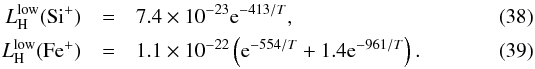 The cooling rate per unit volume due to collisions of element Xi with hydrogen atoms of number density nH is then calculated as
  . The cooling efficiencies due to collisions of O and C+ with neutral hydrogen are taken from Table 4 of Dalgarno & McCray (1972).
To summarize, the total cooling rate at the low-temperature regime is calculated as ![Mathematical equation: \begin{eqnarray} \label{coollow} \Lambda^{\rm low}\left[ {\mathrm{erg \over cm^3~s}} \right]=\sum \limits_i n_{i} n_{\rm H} \xi_{\rm cpw} \left[ L^{\rm low}_{\rm e}(X_i) \, f_{\rm ion} + L^{\rm low}_{\rm H}(X_i) \, \right], \end{eqnarray}](/articles/aa/full_html/2015/07/aa25587-14/aa25587-14-eq160.png) (40)where summation is done over six elements: H, O, C, N, Si, and Fe, where applicable. Here, ξcpw is the cold plus warm gas fraction, and fion = ne/nH is the ionization fraction, the value of which for a given gas temperature Tg is taken from Table 2 of Schure et al. (2009) for the collisionally ionized gas in thermal equilibrium for Tg> 103.8 K. At lower temperatures, fion is set to a constant value of 0.01.
(40)where summation is done over six elements: H, O, C, N, Si, and Fe, where applicable. Here, ξcpw is the cold plus warm gas fraction, and fion = ne/nH is the ionization fraction, the value of which for a given gas temperature Tg is taken from Table 2 of Schure et al. (2009) for the collisionally ionized gas in thermal equilibrium for Tg> 103.8 K. At lower temperatures, fion is set to a constant value of 0.01.
Most of the considered elements (C, Si, Fe, and O) have relatively low critical densities ncrit at which spontaneous and collisional de-excitations become comparable for some transition levels. Cooling due to these elements at nH ≳ ncrit is proportional to nincrit rather than to ninH. We take this into account by multiplying Eq. (40) with ncrit/ (ncrit + nH) and taking ncrit from Table 8 in Hollenbach & McKee (1989). At a low numerical resolution, the critical densities may never be reached.
3.2. High-temperature cooling
For the solar-metallicity plasma with temperature T ≥ 104 K, we adopted the cooling rates of Böhringer & Hensler (1989), which include the line emission for most abundant elements and continuum emission due to free-free, two-photon, and recombination radiation. We have considered nine chemical elements (H, He, C, N, O, Ne, Mg, Si, and Fe), the total (line plus continuum) cooling efficiencies Lhigh(Xi) for which are plotted in Fig. 2 of Böhringer & Hensler (1989). These cooling efficiencies are normalized to nenH and hence need to be multiplied by the ionization fraction fion = ne/nH to retrieve the values that can later be used in our hydro code. The total cooling rates in the high-temperature regime is then calculated as ![Mathematical equation: \begin{equation} \Lambda^{\rm high} \left[ \mathrm{erg \over cm^3~s} \right] = \sum \limits_i L^{\rm high}(X_i) \, f_{\rm ion} \, (n_{\rm H}\xi_{\rm cpw})^2 {n_{i} \,\over n_i^{\rm sol}}, \label{coolhigh} \end{equation}](/articles/aa/full_html/2015/07/aa25587-14/aa25587-14-eq173.png) (41)where ni is the current number density of element i,
(41)where ni is the current number density of element i,  is its number density at the solar abundance, and summation is performed over nine elements: H, He, C, N, O, Ne, Mg, Si, and Fe.
 |
Fig. 2 Cooling efficiency of gas as a function of temperature for the ionization fraction fion = 1.0 but varying metallicity (left panel) and for the gas with solar metallicity but varying ionization fractions fion (right column). |
Figure 2 shows the cooling efficiency laid out in the following form, ![Mathematical equation: \begin{equation} \sum \limits_i {n_i\over n_H} \left[ f_{\rm ion} L^{\rm low}_{\rm e}(X_i) +L^{\rm low}_{\rm H}(X_i) \right] +f_{\rm ion} L^{\rm high}(X_i). \end{equation}](/articles/aa/full_html/2015/07/aa25587-14/aa25587-14-eq177.png) (42)In particular, the left panel has fion = 1, but with varying metallicity, and the right panel has the solar metallicity, but with varying fion. A strong dependence on the metallicity and ionization fraction for fion ≳ 10-3 is evident in the figure.
(42)In particular, the left panel has fion = 1, but with varying metallicity, and the right panel has the solar metallicity, but with varying fion. A strong dependence on the metallicity and ionization fraction for fion ≳ 10-3 is evident in the figure.
3.3. Gas temperature
To use the cooling rates described above, one needs to know the gas temperature T. The latter is calculated from the ideal equation of state P = ρgℛTg/μ, where ℛ is the universal gas constant, using the following expression for the mean molecular weight: 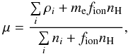 (43)where me is the electron mass and the summation is performed over all nine chemical elements considered in this study.
3.4. Avoiding the overcooling of SN ejecta
When the supernova energy is released in the form of the thermal energy, there may exist the risk of overestimating the gas cooling, which may lead to radiating away most of the released thermal energy. This occurs because the cooling rate Λ is proportional to the square of gas number density, which, for a single-phase medium, may be significantly higher than what is expected in the case of a multiphase medium for the hot supernova ejecta.
To avoid the spurious gas overcooling, we make use of the following procedure. We keep track of the hot SN ejecta by solving for the following equation for the hot gas density ρg,h: 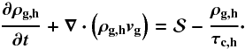 (44)The second term on the r.h.s. accounts for the phase transformation of the hot gas into the cold plus warm (CpW) component, where τc,h = ϵ/ Λh denotes the cooling time of the hot component and the cooling rate Λh is calculated assuming the characteristic cooling efficiency of 5 × 10-23 ergs cm3 s-1 of the hot component with the typical temperature of 108 K (see Fig. 2 and Sect. 6)4.
Equation (44) is solved along with the system of Eqs. (1)−(4) describing the evolution of the gas disk, and the CpW gas fraction is calculated as ξcpw = (ρg − ρg,h) /ρg. We then modify the cooling rates and the SFR by multiplying the total gas density ρg and the hydrogen number density nH in Eqs. (40) and (41) and also in Eq. (30) with ξcpw to retrieve the density of the CpW component. This procedure scales down the cooling rates and the SF rate according to the mass of the CpW component in each computational cell and helps to avoid overcooling and unphysically high SF rates.
3.5. Heating processes
3.5.1. Cosmic ray heating
The cosmic ray heating efficiency is the product of the cosmic ray ionization rate ξcr and the energy input per ionization △ Qcr. We adopt ξcr = 4 × 10-17 s-1 based on the work of Van Dishoeck & Black (1986). The value of △ Qcr is approximately 20 eV. The resulting heating rate due to ionization of hydrogen and helium atoms is ![Mathematical equation: \begin{equation} \Gamma_{\rm cr}=1.34\times 10^{-27} G_0 \left( 0.48 n_{\rm H} + 0.5 n_{\rm He} \right) \left[{\mathrm{ergs} \over \mathrm{cm}^{3}~\mathrm{s}}\right], \end{equation}](/articles/aa/full_html/2015/07/aa25587-14/aa25587-14-eq195.png) (45)where the coefficients 0.48 and 0.5 are taken from Table 6 in Hollenbach & McKee (1989). The quantity G0 represents the interstellar radiation field (IRF) normalized to the solar neighborhood value, i.e., we make here the usual assumption that the cosmic ray intensity scales with the IRF. We calculate its value as G0 = SFRloc/SFRMW, where SFRloc is the local SFR in our models and SFRMW = 1.0 M⊙ yr-1 is the SFR in the Milky Way (Robitaille & Whitney 2010).
(45)where the coefficients 0.48 and 0.5 are taken from Table 6 in Hollenbach & McKee (1989). The quantity G0 represents the interstellar radiation field (IRF) normalized to the solar neighborhood value, i.e., we make here the usual assumption that the cosmic ray intensity scales with the IRF. We calculate its value as G0 = SFRloc/SFRMW, where SFRloc is the local SFR in our models and SFRMW = 1.0 M⊙ yr-1 is the SFR in the Milky Way (Robitaille & Whitney 2010).
3.5.2. Photoelectric heating from small dust grains
The photoelectric emission from small grains induced by FUV photons can substantially contribute to the thermal balance of the interstellar medium at temperatures ≲ 104 K. We use the results of Bakes & Tielens (1994) and express the photoelectric heating rate per unit volume as ![Mathematical equation: \begin{equation} \Gamma_{\rm ph}= 1.0\times 10^{-24} \epsilon_{\rm ph} \, G_0 n_{\rm H} \xi_{\rm d} \,\, \left[ \mathrm{erg~cm}^{-3} \,\mathrm{s}^{-1} \right]. \end{equation}](/articles/aa/full_html/2015/07/aa25587-14/aa25587-14-eq201.png) (46)The photoelectric heating efficiency ϵph is calculated from Fig. 13 of Bakes & Tielens. We also introduced the coefficient ξd = (Md/MHI)/(Md/MHI)⊙ to take a (possibly) different dust to gas mass ratio (Md/MHI) in DGs into account. The latter is found using the following relation between the oxygen abundance (by number density) and the dust-to-gas mass ratio in dwarf galaxies (Lisenfeld & Ferrara 1998):
(46)The photoelectric heating efficiency ϵph is calculated from Fig. 13 of Bakes & Tielens. We also introduced the coefficient ξd = (Md/MHI)/(Md/MHI)⊙ to take a (possibly) different dust to gas mass ratio (Md/MHI) in DGs into account. The latter is found using the following relation between the oxygen abundance (by number density) and the dust-to-gas mass ratio in dwarf galaxies (Lisenfeld & Ferrara 1998):  (47)where the normalization constant Cd = −5.0 is derived from the corresponding quantities of the Small Magellanic Cloud. For the solar dust to gas mass ratio, we adopt (Md/MHI)⊙ = 0.02, typical for the interstellar medium in the solar neighborhood.
4. Solution method
The equations of gas and stellar hydrodynamics are solved in cylindrical coordinates with the assumption of axial symmetry using a time-explicit (except for the gas internal energy update due to gas cooling/heating), operator-split approach similar in methodology to the ZEUS code (Stone & Norman 1992). We use the same finite-difference scheme but, contrary to the ZEUS code, we advect the internal energy density ϵ rather than the specific one ϵ/ρg because the latter may give rise to undesired oscillations in some test problems (e.g., Clarke 2010). Below, we briefly review the numerical scheme. The test results of our implementation of the code are provided in the Appendix.
The solution procedure consists of three main steps. Step 1: we update the gas and stellar components due to star formation and feedback. The corresponding ordinary differential equations describing the time evolution of ρg, ρi, ρgvg, ϵ, ρs, ρsvs, and Πij due to the source and sink terms involving ,  , ,
, ,  , and Γ∗ in Eqs. (1)−(4) and (6)−(8) are solved using a first-order explicit finite-difference scheme. In Step 1, we also calculate the total gravitational potential of the gas and stellar components by solving for the Poisson Eq. (11) using the alternative direction implicit method described in Black & Bodenheimer (1975). The gravitational potential at the outer boundaries is calculated using a multipole expansion formula in spherical coordinates (Jackson 1975). To save on computational time, we invoke the gravitational potential solver only when the relative change in the total (gas plus stellar) density exceeds 10-5 (see Stone & Norman 1992, for details).
Step 2: we solve for the gas hydrodynamics Eqs. (1)−(4), excluding the source and sink terms that have been taken into account in the previous step. The solution is split into the transport and source substeps. During the former, advection is calculated using a third-order accurate piecewise-parabolic scheme of Colella & Woodward (1984) modified for cylindrical coordinates as described in Blondin & Lufkin (1993). During the latter, we update the gas momenta ρgvg due to gravitational and pressure forces and the gas internal energy ϵ due to compressional heating using a solution procedure described in Stone & Norman (1992).
At the end of Step 2, a fully implicit backward Euler scheme combined with Newton-Raphson iterations is used to advance ϵ in time due to volume cooling Λ and heating Γ rates. To monitor accuracy, the total change in ϵ in one time step is kept below 10%. If this condition is not met, we employ local subcycling in a particular cell by reducing the time step in the backward Euler scheme by a factor of two (as compared to the global hydrodynamics time step), and making two individual substeps in the cell where accuracy was violated. The local time step may be further divided by a factor of two until the desired accuracy is reached. The local subcycling help to greatly accelerate the numerical simulations as one need not to repeat the solution procedure for every grid cell.
In Step 2, we also add tensor artificial viscosity to Eqs. (3) and (4) to smooth out strong shocks as described in Stone & Norman (1992). As pointed out in Tasker et al. (2008) and discussed in Clarke (2010), the ZEUS code with the von Neumann & Richtmyer (1950) definition of the artificial viscosity performs poorly on multidimesional tests, such as the Sedov point explosion, yielding nonspherical solutions that may overshoot or undershoot the analytic solution. We demonstrate in Sect. A.2 that using the tensor artificial viscosity and the proper choice of the artificial viscosity parameter C2 = 6 can greatly improve the code performance. However, contrary to the Stone & Norman suggestion to discard the off-diagonal terms of the viscous stress tensor, we demonstrate that in fact these terms should be retained and the most general formulation of the artificial viscosity stress tensor should be used, i.e., ![Mathematical equation: \begin{equation} \label{artviscQ} \mathrm{\bf Q} = \left\{ \begin{array}{ll} l^2 \rho_{\rm g} \boldmath{\nabla} \cdot \boldmath{v}_{\rm g} \left[ \boldmath{\nabla} \boldmath{v}_{\rm g} - \mathrm{\bf e} (\boldmath{\nabla} \cdot \boldmath{v}_{\rm g} )/3 \right] & \,\,\, {\rm if} \quad \boldmath{\nabla} \cdot \boldmath{v}_{\rm g} < 0 \\ 0 & \,\,\, {\rm if} \quad \boldmath{\nabla} \cdot \boldmath{v}_{\rm g}\ge0 \!, \end{array} \right. \end{equation}](/articles/aa/full_html/2015/07/aa25587-14/aa25587-14-eq216.png) (48)where e is the unit tensor, l = C2max(dx), and dx is the grid resolution in each coordinate direction. For the reasons of the code stability, all components of the viscous stress tensor Q should be defined at the same position on the grid, i.e., at the zone centers (contrary to the ZEUS code, which defines the off-diagonal components of rank-two tensors at the zone corners). The Courant limitations on artificial viscosity may be substantial in regions with strong shocks. Therefore, we apply local subcycling (in the same manner as with the internal energy update due to heating/cooling) when the local viscous time step becomes a small fraction of the global hydrodynamics time step.
(48)where e is the unit tensor, l = C2max(dx), and dx is the grid resolution in each coordinate direction. For the reasons of the code stability, all components of the viscous stress tensor Q should be defined at the same position on the grid, i.e., at the zone centers (contrary to the ZEUS code, which defines the off-diagonal components of rank-two tensors at the zone corners). The Courant limitations on artificial viscosity may be substantial in regions with strong shocks. Therefore, we apply local subcycling (in the same manner as with the internal energy update due to heating/cooling) when the local viscous time step becomes a small fraction of the global hydrodynamics time step.
In Step 3, we solve for the stellar hydrodynamics Eqs. (6)−(8), excluding the source and sink terms that have been taken into account during Step 1. The solution procedure is similar to that for the gas hydrodynamics equations, since both systems are defined essentially on the same grid stencil, which is a powerful advantage of the stellar hydrodynamics approach. All components of the velocity dispersion tensor are defined at the cell centers to be consistent with the definition of the stellar artificial viscosity tensor Q. The latter is defined with an analogy to its gas counterpart with the gas density and velocity in Eq. (48) substituted with the stellar density and velocity. Additional terms −∇·Q and −Qik:(∇vs)kj − Qjk:(∇vs)ki have been added to the r.h.s. of Eqs. (7) and (8), respectively, to take the viscous stress and heating due to artificial viscosity into account.
Finally, the global time step for the next loop of simulations is calculated using the Courant condition modified to take star formation and feedback into account. In particular, two time step delimiters of the form,  are added to the usual Courant condition to avoid obtaining negative values of the flow variables. The safety coefficient C3 is set to 0.5. Some modification to the classic Courant condition is required for the stellar hydrodynamics part because the stellar velocity dispersion tensor Π is anisotropic in general. To calculate the stellar hydrodynamics time step, we use the following form:
 ![Mathematical equation: \begin{equation} \triangle t_{\rm st} = \min \left[ {{\rm d}x \over |\boldmath{v}_{\rm s}| +\max \overline{\Pi}_{ii} } \right], \end{equation}](/articles/aa/full_html/2015/07/aa25587-14/aa25587-14-eq223.png) (51)where
(51)where  is the maximum diagonal element of the diagonalized velocity dispersion tensor and the minimum is taken over all grid zones.
Model parameters.
5. The chemodynamical evolution of model dwarf galaxies
Our numerical code has been extensively tested using a standard set of test problems as described in the Appendix. However, even a perfect performance on the standardized tests does not guarantee meaningful results on real problems when all parts are invoked altogether.
Therefore, in this section, we consider the evolution of several representative models of DGs to test the overall code performance and to demonstrate the simulation methodology and recipes described in the previous sections. In particular, we wish to emphasize the effect of stellar dynamics and initial conditions on the simulation outcomes. Moreover, we show the results of simulations with different degrees of rotational support against gravity parameterized by the α-parameter defined as α = vφ/vcirc, where vφ and vcirc are the rotation and circular velocities, the latter being the maximum velocity calculated from the assumption that all support against gravity comes from rotation (i.e., zero gas pressure gradients). We consider three different degrees of rotational support: α = 0.25, 0.5, 0.9. The resulting initial geometries vary from flat-like for large values of α to roundish for small α.
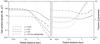 |
Fig. 3 Initial radial profiles of the gas surface density Σg (right) and Toomre Q-parameters (left) in models with different rotational support against gravity as indicated by the α-parameter. The horizontal dotted lines define the critical values of Q-parameter below which star formation is supposed to occur (see the text for more details). |
Our initial configuration consists of a self-gravitating gaseous disk submerged into a fixed DM halo described by a cored isothermal sphere (e.g., Silich & Tenorio-Tagle 2001). We focus on models with a DM halo mass of 109M⊙ and initial gas temperatures of 104 K. We apply the solution procedure described in Vorobyov et al. (2012) to construct self-gravitating equilibrium configurations for different values of α. The initial gas metallicity Zg is set to 10-2Z⊙, the ratio of specific heats γ to 5/3, and the redshift is set to zero. The number of grid zones is 1000 in each coordinate direction, resulting in the effective numerical resolution of 8 pc everywhere throughout the computational domain. We impose the equatorial symmetry at the midplane and the reflection boundary condition at the axis of symmetry. At the other boundaries, a free outflow condition is applied.
Figure 3 presents the initial gas surface density Σg (left panel) and the Toomre Q-parameter (right panel) as a function of the midplane distance in the α = 0.25 model 1 (dash-dotted lines), α = 0.5 model 2 (dashed lines), and α = 0.9 model 3 (solid lines). Evidently, the α = 0.25 model is characterized by the most centrally condensed gas distribution. The horizontal dotted line marks a critical Q-parameter of 1.5 below which star formation is supposed to occur, according to the stability analysis of self-gravitating disks by Toomre (1964) and Polyachenko et al. (1997)5. Evidently, the α = 0.25 and α = 0.5 models are strongly inclined to star formation in the inner 0.5 kpc, while outside this radius the conditions are not favorable because of a rather steep drop in the gas surface density with distance. On the other hand, the α = 0.9 model is characterized by a much shallower profile of Σg, resulting in a significantly larger galactic volume prone to star formation. The parameters of our models are listed in Table 1, where Mg(r ≤ 1 kpc), Mg(r ≤ 3 kpc), and Mg(total) are the gas masses inside a spherical radius of 1 kpc, 3 kpc, and the total gas mass in the computational domain of 8.0 × 8.0 kpc2.
Evidently, the gas mass increases with increasing α, which is explained by the fact that models with higher rotation can support a higher gas mass against gravity of the DM halo. The maximum gas mass is also limited by the action of gas self-gravity (Vorobyov et al. 2012). As the α = 0.5 model demonstrates, switching off the gas self-gravity leads to a factor of two increase in the total gas mass.
When constructing the initial gas density distribution in models 1, 2, and 3, we chose the same “seed” value for gas number density in the galactic center equal to 10 cm-3. We did this to make the initial volume densities and temperatures in the galactic center similar in each model. We could have decreased the seed value in models 2 and 3, trying to adjust the total mass in these models to that obtained in model 1, but then the initial conditions for star formation would also have changed. In addition, it was not clear which mass to take as the reference value because different values are obtained when integrating over different radii because of variations in the radial density profiles.
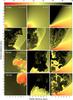 |
Fig. 4 Gas density distribution of three model galaxies differing for the amount of rotational support: the α = 0.25 model 1 (left column), the α = 0.5 model 2 (middle column), and the α = 0.9 model 3 (right column). The time passed from the beginning of numerical simulations is indicated in the leftmost image of each row. The density scale (in cm-3) is shown in the upper strip. |
5.1. The role of α
In Fig. 4 we show a comparison of the gas volume density (ρg) distribution in three model galaxies differing for the value of α. Four representative time snapshots are taken for each model. The α = 0.9 model 3 is characterized by the largest degree of flattening because of the large centrifugal forces. A notable flaring in the initial gas density distribution of model 3 can be seen in the upper right panel. This means that the vertical distribution at R = 0 is characterized by a very steep density and pressure gradient. The overpressurized superbubble created by the stellar feedback preferentially expands along this direction and a bipolar outflow is soon created. The external parts of the disk are not affected by the bipolar outflow and even after t = 150 Myr the gas density of the disk at radii larger than 1 kpc is quite large. Some of the material in the bipolar outflows falls back onto the disk. As a result, the fraction of pristine gas lost by this model is relatively small in spite of the fact that the galactic outflow is very prominent and affects a large fraction of the computational domain. However, the freshly produced metals can be easily channelled out of our model galaxy.
At the other extreme is the α = 0.25 model 1. Here, the initial gas density configuration is almost spherical and the pressure gradient is only slightly steeper in the vertical than in the horizontal direction. A bipolar outflow soon develops, but there is also significant gas transport along the disk and, after 100 Myr, all the gas in the central part of the galaxy (up to a radius of almost 5 kpc) has been completely blown away.
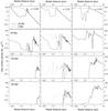 |
Fig. 5 Gas surface density as a function of radius for the same models and at the same moments in time as in Fig. 4. In the upper panels, the initial density distribution is also indicated (dashed lines). The dotted lines in the middle column also show the distribution for the α = 0.5 model without stellar motion (see Sect. 5.2). |
This effect is illustrates in Fig. 5, where the gas surface density as a function of radius is plotted for our three reference models at the same moments in time as in Fig. 4. After 100 Myr there is almost no gas left in the inner 3 kpc in the α = 0.25 model 1, whereas a central hole in the α = 0.9 model 3 is of a much smaller radius, hardly exceeding 0.2 kpc, and the gas distribution at R> 2 kpc is nearly undisturbed. This different galactic evolution, depending on the initial distribution of gas, has been already described in the literature (see in particular Recchi & Hensler 2013), but here we show it in a more realistic context of self-gravitating initial gas configurations.
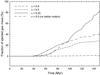 |
Fig. 6 Fraction of ejected gas mass as a function of time for the models with different values of α. The dashed double-dotted line refers to a model in which the stellar motion has been artificially suppressed (see Sect. 5.2). |
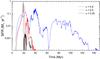 |
Fig. 7 Star formation rates vs. time in three models differing in the value of the centrifugal support α. |
A direct way to appreciate the role of α on the evolution of our model galaxies is to calculate the ejected gas mass for various models. Figure 6 presents the fraction of ejected gas mass vs. time in models 1–3. We find this value by calculating the amount of gas that leaves the computational domain (8 × 8 kpc2) with velocities greater than the escape velocity at the computational boundary. The fraction of ejected mass is very large in the α = 0.25 model because of the blow-away described above, but it is very small for the α = 0.9 model because only a small fraction of the gas originally present in the disk is involved in the galactic outflow. The dash double-dotted line presents the fraction of ejected mass in the α = 0.5 model 2, in which the motion of star was artificially suppressed (see Sect. 5.2 for details.)
The different gas dynamics of the three reference models shown in Fig. 4 also has dramatic consequences for the star formation histories. Figure 7 presents the SFR vs. time. Evidently, the strong star formation feedback in the α = 0.25 model shuts off star formation after ~30 Myr. The α = 0.5 model behaves similarly, although star formation is shut off slightly later. On the other hand, the α = 0.9 model is able to sustain star formation for a longer time, mainly because the disk still remains gas-rich and the conditions for the star formation to occur are fulfilled in many grid cells.
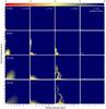 |
Fig. 8 Similar to Fig. 4, but now for the stellar volume density distribution. The scale bar is in M⊙ pc-3. The right-hand column only presents the massive stars. |
Figure 8 presents the distribution of the stellar volume density ρs as a function of time and for the same models and at the same time instances as in Fig. 4. In addition, the right-hand column presents the volume density of high-mass stars . We can clearly see that the stellar distribution in the α = 0.25 model is more homogeneous and isotropic than in the α = 0.9 model, wherein many stars tend to be located along the polar axis. Owing to a preferable concentration of gas toward the midplane in the α = 0.9 model, however, a significant fraction of stars is also distributed near the midplane, constituting a stellar disk. This effect is much less evident for the models with α = 0.5 and α = 0.25. To quantify this, we calculated the fraction of the total stellar mass confined within a vertical height of 1 kpc and 2 kpc. It turns out that in the α = 0.25 model these values are 37% and 62%, respectively, whereas in the α = 0.9 model they are 90% and 94%, indicating a much more compact stellar distribution in the higher-α model. Finally, a comparison of the distribution between ρs (the total stellar density) and in the α = 0.9 model indicates that stars are preferentially forming at low galactic altitudes ≲ 1 kpc, but are later spread out owing to their own initial dispersion (5 km s-1) and, especially, owing to significant bulk velocities inherited from parental gas clouds. The off-plane star formation is taking place predominantly in dense gaseous clumps and on the cavity walls.
5.2. The role of the stellar motion and the initial gas distribution
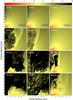 |
Fig. 9 Time evolution of the gas volume density in three models with α = 0.5. The l.h.s. column presents the time evolution in model 2, already shown in Fig. 4. The middle column shows model 4, in which the motions of stars are artificially suppressed. In the r.h.s. column we show model 5, for which the initial equilibrium distribution was constructed without taking gas self-gravity into account. Note the different evolutionary times in the latter model. |
We employ the moments of the collisional Boltzmann equation to describe the motion of stars. In addition, we start our simulations from self-consistent initial equilibrium conditions that were built taking gas self-gravity into account. In some studies, the initial configuration is constructed without taking gas self-gravity into account, although during the dynamical evolution the gas self-gravity may be included. It is instructive to study how these two new recipes affect the dynamics of our model galaxies.
In Fig. 9 we show the gas volume density in three models with α = 0.5 at four representative evolution times. In particular, the left-hand column shows the evolution of our reference model 2, already shown in Fig. 4. The middle column shows model 4, in which the stellar dynamics has been artificially suppressed. Stars are allowed to form, but they are effectively motionless and are fixed to their birthplaces until they die. Evidently, the final gas distribution in model 4 is clumpy: the galactic volume is filled with moving cometary-like clouds. The increase in the number of clumps is caused by a reduced feedback in the absence of stellar motion. The moving clumps leave behind the newly born stars so that part of the stellar energy is released outside the clumps, which makes it easier for the clumps to survive. In the presence of stellar motion, the newly born stars follow the gas clumps (at least for some time) because they inherit gas velocity at the formation epoch, releasing the stellar energy inside the clumps and dispersing most of them.
The final gas distribution in model 2 is smooth and shows no cometary-like structures. At the same time, the outflow in model 4 clears a larger hole near the midplane than in the reference model. The combination of these two effects results in a rather chaotic gas surface density distribution shown in the middle panel of Fig. 5 with dotted lines. Model 4 is characterized by a somewhat higher star formation feedback, as is indicated by the fraction of ejected gas mass shown by the dot-dot-dashed line in Fig. 6.
The increased feedback in the model without stellar motions is likely because the energy of both supernova explosions and stellar winds is released in regions characterized by a systematically higher temperature and lower density than in the reference model. This is because star formation creates regions of slightly lower density compared to the surrounding gas, and stellar winds stir and heat up the circumstellar gas. If stars are motionless, then their feedback is confined to their birthplaces. On the other hand, if stellar motion is allowed, stars can move to neighboring regions, where the density is likely to be higher and where stellar winds have not yet heated the gas. The feedback will be thus less effective. This conclusion is at variance with that of Slyz (2007), who showed that stellar motion makes the feedback more effective and can even solve the overcooling problem. This different outcome is probably because of the lack of feedback from stellar winds in Slyz’s models.
Figure 10 presents the stellar volume density distributions for the same models as in Fig. 9. The left-hand column corresponds to the reference model 2, already shown in Fig. 8, while the middle column presents model 4, in which stellar motions are suppressed. Evidently, models with and without stellar motion produce strikingly different stellar distributions. The stellar distribution in the reference model is rather smooth, whereas in the model without stellar motions most of the stellar content is confined to the midplane and the inner region. In fact, the fraction of the total stellar mass confined within a vertical height of 0.3 kpc (from the midplane) is 82% for the reference model, but this value increases to 98% for the model without stellar motions. The curious stellar stripes visible in the middle column are caused by the development of a gaseous supershell: many stars tend to form on the walls of this supershell and, as a consequence, their position reflects the shell’s expansion. The lack of stellar motion makes these structures permanent. The fact that these structures are not observed in real galaxies outlines the importance of a proper treatment of stellar dynamics in numerical simulations of DGs.
Finally, we investigate the question of how the choice of the initial gas density distribution can influence the subsequent evolution of dwarf galaxies. For this purpose, we choose α = 0.5 and construct two initial gas density distributions: one taking gas self-gravity into account and the other without it. To compare the models with and without-self gravity easier, we require that the gas mass within the 3-kpc radius be similar in both models. The model with the initial equilibrium distribution taking gas self-gravity into account is in fact our model 2 considered above, while its counterpart is further referred as model 5 (see Table 1 for model parameters).
The initial radial profiles of the gas surface density and the Toomre Q-parameter in model 5 are shown in Fig. 3 by the dash-dot-dotted lines. Not surprisingly, the initial gas distribution in model 2 is more centrally condensed than in model 5: gas self-gravity creates an additional gravity pull toward the galactic center6, resulting in a denser initial configuration. For instance, the total gas mass in the inner sphere of 1 kpc in the initial model without self-gravity is ≈ 107M⊙, while this value rises by a factor of 2.8 in the model with self-gravity. As a consequence, the Toomre Q-parameter is initially greater than 2.0 everywhere and star formation is effectively suppressed.
The right-hand column in Fig. 9 presents the gas volume density distribution in model 5. We emphasize that the gas self-gravity in this model is only neglected when building the initial distribution; in the subsequent evolution the gas self-gravity is however turned on again. Evidently, the evolution of model 5 is notably slower owing to the fact that star formation is initially suppressed. The gas cools and contracts, and only after 120 Myr the conditions for star formation become favorable in the galactic center, whereas a vigourous star formation feedback is seen in model 2 already after 50 Myr of the evolution. The initial slow start in model 5 is consistent with a long dynamical timescale in this model. For the mean gas volume density in the inner 1 kpc of 4 × 10-25 g cm-3, the corresponding free-fall time in model 5 is approximately 110 Myr, which is consistent with the time epoch of the first star formation episode in this model. Because of significant thermal support and radially increasing dynamical timescale (density drops with radius), it takes several dynamical timescales to adjust to a state similar to that of model 2. By the end of simulations in model 5 (800 Myr), the outflow is still not as strong as in its counterpart model 2 and the central gap has not yet developed.
The right-hand column in Fig. 10 presents the stellar volume density distribution in model 5. A visual inspection of the l.h.s. and r.h.s. models reveals that the stellar distributions in models 2 and 5 are in general similar (but note the difference in ages 150 vs. 800 Myr), though the stars in the latter model are distributed somewhat more irregularly. By the end of numerical simulations, the total mass of formed stars in the 800-Myr-old model 5 is still a factor of 4 lower than in the 150 Myr-old model 2, highlighting a much slower evolution in the model that starts from a non-self-consistent initial configuration, i.e., without initial gas self-gravity.
6. Discussion and model caveats
We did not aim for a detailed comparison of our numerical simulations with observed DGs, which is our task for subsequent studies. Instead, we chose three typical models for DGs with different rotational support against gravity to test the code performance on global simulations, and not just on a predefined set of classic test problems. The current version of the code assumes axial symmetry and neglected chemical reactions, which leaves the door open for future improvements. At the same time, we managed to develop an efficient mathematical recipe for describing the phase transition from stars into gas using the continuity equation for the mean stellar age (see Sect. 2.6).
We chose some simulation parameters without a detailed parameter study or without an in-depth analysis. We avoid this kind of detailed study for the sake of clarity and to make the paper more concise and readable. A deeper parameter study will be performed in follow-up papers. It is nevertheless important to point out the following potential caveats in the choice of some parameters:
-
ϵsw(see Sect. 2.7.3.): massive and intermediate-mass stars expel a significant fraction of their mass by stellar winds. Although their lifetimes shorten with mass, the mass-loss rates increase disproportionately, so that for solar abundances the total wind energy of most massive stars exceeds that of SNeII over the stellar lifetime. For radiation-driven HII regions, Lasker (1967) stated that the ISM is only heated a very low amount and derived analytically an efficiency of 1%, because the ionizing radiation energy is almost instantaneously lost by line emission and only the expansion of HII regions steers up the surrounding ISM. Although the additional wind power amounts to almost 10% of the radiation energy, it is expected to deposit a larger fraction as the thermal and kinetic ISM energies. Since in most chemodynamical simulations (Theis et al. 1992; Samland et al. 1997) the Ly continuum radiation is applied with an efficiency of 10-3, ϵsw is assumed to 100%. This value is also used here.
-
ϵSN(see Sect. 2.7.1): for the thermalization efficiency of the SNII explosion, i.e., the fraction of the explosion energy transferred to gas thermal energy, we have adopted the value ϵSN = 1.0 for simplicity and to avoid further parameter studies. The thermalization efficiency has been subject to considerable studies in the past. Thornton et al. (1998) performed single 1D supernova explosion models and derived ϵSN = 0.1. Estimates from cumulative SNII explosions, forming superbubbles, suggest a significant dependence of ϵSN on the temperature and density of the external medium (Recchi et al. 2001; Recchi 2014). A different approach, where the contribution of a whole stellar population is considered (Melioli & de Gouveia Dal Pino 2004) clearly shows that ϵSN is a function of time. We performed a test simulation adopting ϵSN = 0.1. The extent of the galactic winds was reduced in this case, but not by a large factor. In fact, a great deal of self-regulation is achieved with our formulation for the SFR (see Eq. (30)). Further, the larger ϵSN, the larger the heating of the surrounding medium, and the higher the probability that the star formation is quenched for a period of time (see Koeppen et al. 1995, for more details on self-regulated star formation). Thus, although we plan to make more careful selection of ϵSN in follow-up papers, this parameter does not appear change the results of the simulations drastically.
-
ncr (see Sect. 2.7.4): the threshold density above which star formation is allowed, ncr = 1 cm-3 has been chosen in compliance with other numerical studies (Springel & Hernquist 2003; Recchi et al. 2007). Also in this case, many different values for ncr have been chosen in the literature and detailed studies on the effect of this parameters have been performed. In the framework of ΛCDM cosmological simulations, ncr of 0.1 cm-3 is generally used (Katz 1992) and its effect on the star formation was studied, e.g., by Kay et al. (2002), but also applied to much larger resolutions of smooth-particle hydrodynamics applications (Stinson et al. 2006). It appears that an extremely large value of (up to 100 cm-3Governato et al. 2010) is required to reproduce the observed structural properties of DGs (but see also Pilkington et al. 2011). Quite generally, the star formation density threshold should be set based on the density at which gravitational instabilities can be resolved (see, e.g., Truelove et al. 1997). This leads, for instance, Stinson et al. (2013) to assume a threshold of 9.3 cm-3 based on their adopted resolution. Clearly, our choice of ncr is simplistic and deeper studies are required in follow-up publications. In our simulation, only a tiny fraction of gas reaches densities larger than a few tens of cm-3, therefore the adoption of very large values of ncr would lead to extremely localized and sporadic star formation. The very large feedback achieved in the simulations of Governato et al. (2010) is certainly able to produce modeled DGs with structural properties similar to those observed, but it is not clear whether the chemical properties can be equally well reproduced. A large amount of feedback can create galactic winds, which are able to expel the large majority of metals that are freshly produced in the galaxy, thus at the end of the evolution the model galaxy should be almost deprived of heavy elements.
-
Λh (see Sect. 3.4): the cooling function typical of hot gas Λh, which has been used to calculate the cooling timescale of the hot SN ejecta, has been estimated based on a temperature of the hot ejecta of 108 K. It must be admitted that this temperature only holds just after the SN explosion, but the ejecta cools significantly afterward. Nevertheless, the thermal SN energy has been varied artificially to probe its influence on galactic winds (Dalla Vecchia & Schaye 2012). However, we are in the cooling regime dominated by bremsstrahlung, and the temperature dependence of the cooling function is not so severe (the cooling is approximately proportional to
 in this temperature range).
7. Conclusions
We presented the stellar hydrodynamics approach for modeling the evolution of DGs, paying special attention to the co-evolution of gas and stars. The distinctive feature of our models is how we treat the stellar component. Unlike many previous studies that use various versions of the N-body method to compute the dynamics of stars, we employ the stellar hydrodynamics approach based on the moments of the collisionless Boltzmann equation, originally introduced by Burkert & Hensler (1988), and applied and further developed by Theis et al. (1992), Samland et al. (1997), Vorobyov & Theis (2006, 2008), Mitchell et al. (2013), Kulikov (2014). For the first time, we provided an effective mathematical recipe for describing the death of stars in the framework of stellar hydrodynamics using the concept of a mean stellar age. We performed an extensive testing of our numerical scheme using classical and newly developed test problems, paying particular attention to the proper recipe for artificial viscosity to achieve the best agreement with the analytical solution for the Sedov test problem.
We demonstrate the success of our numerical approach by simulating the evolution of three DGs differing in the amount of rotation described by the spin parameter α = 0.25, α = 0.5, and α = 0.9. In agreement with previous studies, models with low values of α are characterized by stronger outflows, ejecting a larger amount of gas from the galaxy. This is because the initial gas distribution in the low-α models is almost spherical, so that the gas pushed by the stellar feedback expands almost isotropically. In contrast, models with high values of α exhibit a disk-like initial gas distribution with a pronounced radial flaring. The pressure gradient in the vertical direction in these models is very steep, which favors the development of bipolar galactic outflows. The transport of gas in the horizontal direction (i.e., along the galactic midplane) is very limited, and therefore this model is able to keep most of the initial gas bound to the galaxy. The fraction of ejected gas (i.e., the fraction of gas that leaves the computational domain with a speed higher than the escape speed) is only a few percent for the α = 0.9 model, but it raises to 80% for the model with α = 0.25.
At the same time, models with a low value of α produce a more diffuse stellar population than models with higher α. Only models with α ≥ 0.5 reveal the formation of a definite stellar disk component. We demonstrate the importance of the stellar dynamics by artificially turning off stellar motions. In this case, the resulting stellar population is mostly concentrated to the midplane and shows stripe-like structures emanating from the galactic center, which are not observed in real galaxies.
Stars start heating the natal gas almost instantaneously owing to the effect of stellar winds neglected in many recent hydrodynamical simulations. We found that if stellar dynamics is suppressed, Type II supernovae (the main source of mechanical feedback) explode in a medium heated and diluted by the stellar winds. In this kind of an environment, radiative losses are small and the supernova feedback is extremely effective. If, on the other hand, stellar motions are allowed, they can move from the natal site (where the gas has been heated and stirred by the effect of stellar winds) to neighboring regions before exploding as supernovae. These regions are characterized by lower temperatures and higher densities, so that the supernova feedback becomes less effective. It is thus crucial to correctly simulate stellar dynamics (together with all relevant sources of feedback) to study the interplay between stars and the interstellar medium.
Unlike many other studies of DGs, we used the self-consistent initial gas configuration that was constructed taking the gas self-gravity into account (Vorobyov et al. 2012). This gas configuration is usually more centrally condensed and prone to star formation than that constructed neglecting gas self-gravity. We compared the evolution of our model galaxy starting from these different initial configurations and found that models that start from non-self-gravitating initial configurations evolve much slower than those that start from self-gravitating configurations. In the former, a major episode of star formation and the development of prominent outflows may by delayed by 0.5−0.8 Gyr as compared to the latter. This is exclusively the effect of initial conditions (or, better to say, the effect of using non-self-consistent initial gas configurations), because the gas self-gravity is turned on in both models once the evolution has started.
In the future, a detailed comparison of our stellar hydrodynamics simulations with a more conventional N-body treatment of stellar dynamics is desirable to assess the weak and strong sides of the Boltzmann moment equation approach.
Online material
Appendix A: Testing gas hydrodynamics equations
Our numerical scheme for solving the equations of gas hydrodynamics (1)–(4) can be tested using a conventional set of test problems suitable for cylindrical coordinates. Below, we provide the results of six essential test problems, each designed to test the code performance at various physical circumstances. The code has also performed well on two additional tests: the two interacting blast waves and the Noh (or implosion) problems, but we do not provide the results for the sake of conciseness.
Appendix A.1: Sod shock-tube test
This test is often used to assess the ability of a numerical algorithm to accurately track the position of relatively weak shock waves and contact discontinuities. Initial conditions involve two discontinuous states along the z-axis, with a hot dense gas on the left and cold rarified gas on the right. More specifically, we set the pressure and density at z ∈ [ 0−0.5 ] to 1.0, while at z ∈ [ 0.5−1.0 ] the pressure is 0.1 and density is 0.125. The velocity of a γ = 1.4 gas is initially zero everywhere.
Filled circles in Fig. A.1 show the results of the Sod shock-tube test computed with a resolution of 200 grid zones and C2 = 4 (the number of zones over which the shock is spread), while the solid lines plot the analytic solution at t = 0.235. It is evident that the code tracks well the positions of shock waves and contact discontinuities, which are resolved by 3–4 zones, in accordance with the chosen value of C2. Decreasing C2 results in sharper shocks and contact discontinuities but may increase the magnitude of anomalous spikes in the specific energy (bottom-right panel), and hence is not recommended. Increasing C2 to 6 produces results similar to those for C2 = 4, except that the shocks and contact discontinuities are now resolved by 5−6 zones.
Appendix A.2: Sedov point explosion
The Sedov explosion problem tests the code’s ability to deal with strong shocks. In contrast to the Sod shock-tube test, in which shock waves were of a pure planar geometry, this test involves a spherically symmetric strong shock wave. Hence, the point explosion is a powerful test on the code’s ability to render spherically symmetric structures on an essentially nonspherical grid stencil.
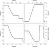 |
Fig. A.1 Sod shock tube problem for the gas density (upper-left), velocity (upper-right), pressure (lower-left), and specific internal energy (lower-right). The numerical solution is shown by open circles, while the analytical one is plotted by solid lines. |
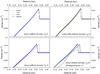 |
Fig. A.2 Sedov point explosion test for the explosion energy 1051 erg and background density n = 0.01 cm-3. The analytic solution is shown by the red lines, while the numerical solutions along the z-axis, r-axis, and diagonal z = r are shown by the black, pink, and blue lines, respectively. The top left panel presents the solution for the tensor artificial viscosity with C2 = 6 ; the top right panel, for the scalar artificial viscosity and C2 = 3; the bottom left panel, for the tensor artificial viscosity and C2 = 3; and the bottom right panel, for the tensor artificial viscosity with off-diagonal terms set to zero and C2 = 6. |
To initialize the explosion, we consider a cold (T = 10 K) homogeneous medium with number density n = 10-2 cm-3 and inject 1051 ergs of thermal energy (equivalent to one supernova) into the innermost grid cell. The adopted resolution is 300 × 300 grid cells and the size of each cell is 1.0 pc in each coordinate direction (z and r). We do not inject energy into a central sphere comprising a few cells near the coordinate origin, which is the usual practice to alleviate the problem of a nonspherical geometry. Instead, we consider the most difficult situation when energy is injected in just one, essentially cylindrical innermost cell.
Figure A.2 compares our derived density distributions along the z-axis (black line), the r-axis (pink line), and the diagonal z = r (blue line with circles) with the analytic solution given by the red line (Sedov 1959) at t = 1 Myr after the explosion. In particular, numerical simulations in the top left panel are obtained using the tensor artificial viscosity (AV) as defined in Sect. 4, while the density distribution in the top right panel is obtained using the “classic” scalar AV, as described by Richtmyer & Morton (1995). It is evident that the tensor AV yields a much better agreement with the analytic solution. The expanding shell has almost a perfect spherical shape (all three lines showing the numerical solution virtually coincide), notwithstanding the fact that the energy was injected into a cylindrically shaped innermost cell. On the other hand, the Richtmyer & Morton scalar AV yields a notable deviation from sphericity along the r and z axes, as seen in the top right panel of Fig. A.2. The Richtmyer & Morton solution also slightly overshoots the analytical solution. Regardless of the AV prescription used, the shock front is resolved by 2−3 grid zones.
We want to emphasize that all components of the artificial viscosity tensor Q should be used, including the off-diagonal terms. Neglecting the latter, as is done in, e.g., Stone & Norman (1992), leads to a significant deterioration of the numerical solution. The bottom right panel in Fig. A.2 demonstrates the effect of zeroing the off-diagonal terms in Q. As one can see, the numerical solution is skewed, notably undershooting the position of the shock front in the r-direction and along the diagonal direction but reproducing the shock front rather well in the z-direction.
A caution should be paid when choosing the AV softener C2. As one can notice in Fig. A.2, the test was done with different values of C2 for the tensor and scalar AV, 6 and 3, respectively. If we choose C2 = 3 for the tensor AV, the position of the shock front notably undershoots the analytic solution, as is illustrated in the bottom left panel of Fig. A.2. Fortunately, once the proper value of C2 is found, the tensor AV algorithm performs well regardless of the energy input, background density, or numerical resolution. We demonstrate this in Fig. A.3 showing the tensor AV performance for various choices of the input parameters as indicated in each panel and C2 = 6. It is evident that the test results are virtually insensitive to a particular choice of initial conditions.
The sensitivity of the Sedov test to a particular choice of the AV softener C2 is a well-known problem of numerical codes that evolve the internal energy (e.g., Tasker et al. 2008). Switching to the total energy helps to eliminate this problem (e.g., Clarke 2010). However, in numerical codes that make use of a staggered grid as our own, with vector and scalar variables defined at different positions on the grid, solving for the total energy equation is not a good option as it inevitably requires interpolating between the internal and kinetic energies to obtain the total energy (Clarke 2010) or applying corrections after each time step to conserve the total energy (Vshivkov et al. 2011). In either case, this practice, according to our experience, often comes at a cost of degraded performance on other test problems and is not recommended. Instead, we show that a proper choice of the artificial viscosity softener can help to resolve this problem without resorting to the total energy equation.
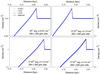 |
Fig. A.3 Sedov point explosion test for various explosion energies, background densities, and numerical resolutions as indicated in each panel. The tensor artificial viscosity with C2 = 6 is used for every plot. The line meaning is the same as in Fig. A.2. |
Appendix A.3: Collapse of a pressure-free sphere
The gravitational collapse of a pressure-free sphere is used to assess the code’s ability to accurately treat converging spherical flows in cylindrical coordinates. This test is also useful for estimating the performance of the gravitational potential solver on dynamical problems (our solver does well on the static configurations such as spheres and ellipsoids). To run this test, we set a cold homogeneous sphere of unit radius and density (for convenience, the gravitational constant is also set to unity) and let it collapse under its own gravity. The analytic solution to this problem only exists in the limit of an infinite cloud radius, describing the collapse of every mass shell (Hunter 1962). In the cylindrical geometry, however, we consider a cloud of finite radius with a sharp outer boundary to preserve the cloud sphericity. As a result, a rarefaction wave develops after the onset of the collapse, propagating toward the coordinate origin and necessitating complicated corrections to the analytic solution (Truelove et al. 1998).
The left panel in Fig. A.4 compares the results of our numerical simulations with the “uncorrected” analytic solution of (Hunter 1962, red line) at t = 0.535 (or 0.985 that of the free-fall time) when the initial density has increased by nearly three orders of magnitude. As in the previous test, we plot the numerically derived density along the z-axis (black line), r-axis (green line), and the z = r diagonal (blue line with circles). The numerical resolution is 200 × 200 grid zones. The cloud’s outer boundary is somewhat smeared out because of the action of the rarefaction wave. The peak density is also about 1% smaller than that predicted from the analytic solution. On the other hand, the code performs well on preserving sphericity of the collapsing cloud. In the right panel, we turn off the volume averaging corrections applied to the advection of the r-momentum in the r-direction as described in Blondin & Lufkin (1993), which results in the development of an artificial density spike near the z-axis and also in the distortion of a spherically symmetric collapse. This test demonstrates the utility of the volume averaging corrections introduced originally by Blondin & Lufkin (1993) in the PPA advection scheme in non-Cartesian coordinates.
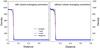 |
Fig. A.4 Collapse of a pressure-free sphere showing the gas density at 0.985 that of the free-fall time. The left and right panels show the test results with and without the volume averaging corrections as described in Blondin & Lufkin (1993). The line meaning is the same as in Fig. A.2. |
Appendix A.4: Collapse of a rotating sphere
This test is invoked to assess the code’s ability to conserve angular momentum. The setup consists of a isothermal (T = 10 K) homogeneous sphere of unit radius and density, which rotates at a constant angular velocity Ω0. The latter is found from the requirement that the ratio β of the rotational energy  to gravitational energy
  is equal to 5%. Here, I = 2M0R2/ 5 is the moment of inertia of a homogeneous sphere of radius R and mass M0. The adopted value of β = 0.05 is close to an upper limit found in rotating prestellar molecular cloud cores and DM halos.
In the absence of any mechanisms for angular momentum redistribution, the mass with specific angular momentum less than or equal to K = ωr2, where ω is the angular velocity at a distance r from the z-axis, should be conserved and equal to (Norman et al. 1980), ![Mathematical equation: \appendix \setcounter{section}{1} \begin{equation} \label{angmom} M(K)=M_0 \left[ 1 - \left(1- {K \over \Omega_0 R^2 } \right)^{3/2} \right]. \end{equation}](/articles/aa/full_html/2015/07/aa25587-14/aa25587-14-eq308.png) (A.1)A deviation from Eq. (A.1) would manifest the nonconservation of angular momentum in the numerical algorithm.
(A.1)A deviation from Eq. (A.1) would manifest the nonconservation of angular momentum in the numerical algorithm.
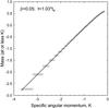 |
Fig. A.5 Specific angular momentum spectrum M(K), calculated using Eq. (A.1), for a collapsing sphere at 1.03tff. The analytic spectrum is shown with the solid line, while the test results are plotted with open circles. |
The solid line in Fig. A.5 shows the initial mass spectrum M(K), whereas the open circles present the mass spectrum obtained at time 1.03 × tff = 0.551, where tff is the free-fall time for a nonrotating sphere of the same density and radius. The numerical resolution is 200 × 200 grid zones. By t = 0.551, the density near the center of the sphere has increased by more than three orders of magnitude, but the deviation of the mass spectrum from the initial configuration is negligible everywhere except at lowest values of K. This deviation is a manifestation of angular momentum nonconservation near the rotational axis caused by imperfections in the interpolation procedure across the inner r-boundary. Nevertheless, the total mass of gas that suffers form the angular momentum nonconservation is just below 1%, and therefore should not affect notably the global evolution.
Appendix A.5: Kelvin-Helmholtz instability
The Kelvin-Helmholtz instability (KHI) occurs at the interface between two fluid moving with different velocities. In the context of this paper, this instability operates at the interface between the hot supernova ejecta and the cold swept-up shell and may cause an accelerated disintegration of the latter (e.g., Vorobyov & Basu 2005). Therefore, it is essential that the code be able to demonstrate the development of the KHI as expected from the linear perturbation theory.
The initial setup involves two fluids moving in opposite directions along the z-axis with the relative velocity vz,rel = 0.2cs, where cs = 0.06 is the sound speed. The interface between the fluids is located at r = 0.5 and the densities of the inner and outer fluids are ρin = 1.0 and ρout = 0.1, respectively. We use periodic boundary conditions and the resolution is 200 × 200 grid zones on the 1.0 × 1.0 computational domain.
To trigger the instability, we impose a sinusoidal perturbation on the radial velocity vr of the form 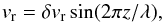 (A.2)where the amplitude and wavelength of the perturbation are δvr = vz,rel/ 100 and λ = 1/6, respectively. The perturbation is applied to five neighboring grid zones on both sides of the fluid interface.
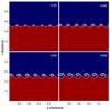 |
Fig. A.6 Development of the KHI at different moments in time (see text for more detail). |
Figure A.6 demonstrates the growth of the KHI with time. There are six growing vortices, in agreement with the wavelength of the perturbation λ = 1/6, and the growth time is approximately 50−60, again in agreement with the characteristic growth time of the KHI for our choice of the fluid density and velocity, 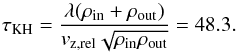 (A.3)We should note here that, for this particular test, gravity can be neglected. Therefore, all modes of perturbation, irrespective of their wavelengths (or wavenumbers) are unstable (see Vieser & Hensler 2007, for stability criteria when gravity is taken into account).
Appendix A.6: Overstability of a radiative shock
A useful test problem for hydrodynamic codes with optically thin radiative cooling is described in Stone & Norman (1993). The test involves setting a unform flow of gas with velocity v0 against a reflecting wall. An adiabatic reflection shocks forms immediately at the wall and propagates upstream with velocity vsh = v0/ 3. After approximately one cooling time, the shock loses its pressure support and is then advected back to the wall at vsh ≲ −v0. After reflecting off the wall, the shock again becomes adiabatic and propagates outward to repeat the cycle.
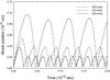 |
Fig. A.7 Shock position versus time of a one-dimensional radiative shock during overstable oscillations. The shock positions for the flow velocities of 120 km s-1, 130 km s-1, and 150 km s-1 are plotted with solid, dash-dotted, and dotted lines, respectively. |
Figure A.7 presents the test results for the cooling function with solar metallicity and ionization fraction fion = 10-3. Gas heating is turned off for this test. The initial setup is identical to that described in Stone & Norman (1993), i.e., the initial gas number density and temperature are set to 10 cm-3 and 104 K, respectively. The position of the shock front for three flow velocities of 120 km s-1, 130 km s-1 and 150 km s-1 are plotted with the solid, dash-dotted, and dashed lines, respectively. The shock position demonstrates regular pulses, as expected. The amplitude and period of the observed oscillations are somewhat different from those presented in Stone & Norman (1993), which simply reflect the difference in the adopted cooling functions. The upstream velocity of the adiabatic shock is close to the expected value, v0/ 3. For instance, in the case of v0 = 150 km s-1, the maximum upstream velocity of the shock is 47 km s-1. This test demonstrates the reliability of our solution scheme for the gas cooling and heating described in Sect. 3.
Appendix B: Testing stellar hydrodynamics equations
Testing the stellar hydrodynamics Eqs. (6)−(8) presents a certain challenge since stellar systems are described by a stellar dispersion tensor, which may be anisotropic, rather than by an isotropic pressure. Fortunately, some of the test problems considered above can be adapted to stellar hydrodynamics as well. The matter is that the equations of stellar hydrodynamics can be formally made identical to those of gas hydrodynamics for a specific set of initial conditions (note that the continuity equations are always identical). Indeed, for a one-dimensional flow along the z-direction (with zero gravity and no star formation), Eqs. (7) and (8) become 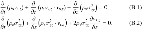 These equations become identical to the corresponding gas dynamics equations for ρgvz and ϵ, if we set
  ,
,  , and γ = 3 (see Mitchell et al. 2013, for details). This fact allows us to directly compare the performance of both stellar and gas hydrodynamics code on some test problems considered in Sect. A or use analytic solutions available from the gas dynamics.
Appendix B.1: Sod shock-tube test
The initial setup for this test is identical to that considered in Sect. A.1. We run the test along the z-axis and set  and ρs at z ∈ [ 0−0.5 ] to 1.0, while at z ∈ [ 0.5−1.0 ] the z-component of the stress tensor is 0.1 and stellar density is 0.125.
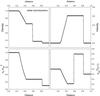 |
Fig. B.1 Sod shock-tube problem for the stellar density (upper-left), velocity (upper-right), z-component of the stress tensor (lower-left), and square of the z-velocity dispersion (lower-right). The numerical solution is shown by open circles, while the analytical solution is plotted by solid lines. |
Our numerical results for C2s = 4 and t = 0.14 (open circles) are compared against the analytical solution (solid lines) in Fig. B.1. It is seen that our numerical scheme correctly reproduces the position of shock waves and contact discontinuities in the stellar fluid. On the other hand, small-scale oscillations are evident at shock positions, perhaps reflecting the lack of energy dissipation due to the collisionless nature of stellar hydrodynamics. An increase in the coefficient of artificial viscosity helps to reduce the amplitude of spurious oscillations but simultaneously increases the shock smearing and hence is only recommended if these oscillations lead to numerical instabilities.
Appendix B.2: Collapse of a cold sphere and angular momentum conservation
The collapse of a cold stellar sphere, both with and without rotation, produces very similar results to those presented in Sects. A.3 and A.4 and will not be repeated here. This ensures that our stellar hydrodynamics part is expected to perform well on problems involving gravitational contraction/expansion with and without rotation.
Appendix C: Testing the chemical evolution routines
It is currently common to find hydrodynamical codes coupled with passive scalars (or other numerical techniques), which are able to follow the evolution of the metals in a simulation. However, usually no test is performed to check the numerical accuracy of these routines. Actually, since a very vast literature on analytical solutions of the chemical evolution of galaxies and other astronomical objects exists (see, e.g., Tinsley 1980; Matteucci 2001; Hensler & Recchi 2010, and references therein) it is indeed not difficult to benchmark the chemical evolution routines of a chemodynamical code.
The “closed box” model of chemical evolution is based on the following assumptions: (i) the system is uniform and closed (there are no inflows or outflows); (ii) the IMF does not change with time; (iii) the gas is well mixed at any time; and (iv) stars more massive than a certain threshold mass Mthr die instantaneously whereas stars less massive than Mthr live forever. This last assumption, although very restrictive, is fulfilled if we look at specific chemical elements, in particular O and the other α-elements, since they are mostly synthesized by Type II SNe and the (long-living) low- and intermediate-mass stars contribute negligibly to their production.
In a system made up of only gas and stars (DM does not play any role here) we define the quantities, ![Mathematical equation: \appendix \setcounter{section}{3} \begin{eqnarray} \label{eq:r}&&R =\int_{M_{\rm thr}}^\infty \left[M-M_{\rm rem}(M)\right]\phi(M){\rm d}M, \\ \label{eq:yo}&&y_{\rm O}=\frac{1}{1-R}\int_{M_{\rm thr}}^\infty M p_{\rm O}(M)\phi(M){\rm d}M, \end{eqnarray}](/articles/aa/full_html/2015/07/aa25587-14/aa25587-14-eq345.png) where Mtot = Mgas + Mstars, Mrem(M) is the remnant mass after a star of mass M has died and MpO(M) is the oxygen mass newly synthesized by the star of mass M (pO(M) is the true yield of O). Under the initial condition Mgasf(0) = Const. = Mtot, Mstars(0) = 0, XO(0) = X0 we find that
where Mtot = Mgas + Mstars, Mrem(M) is the remnant mass after a star of mass M has died and MpO(M) is the oxygen mass newly synthesized by the star of mass M (pO(M) is the true yield of O). Under the initial condition Mgasf(0) = Const. = Mtot, Mstars(0) = 0, XO(0) = X0 we find that 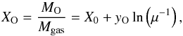 (C.3)
(C.3)
where μ = Mgas/Mtot. This is the famous analytical solution of the closed box model, which only depends on the gas fraction μ.
We have integrated numerically Eqs. (C.1) and (C.2) by using the values of Mrem(M) and MpO(M) tabulated by Woosley & Weaver (1995), using Z = 0.01Z⊙ as initial metallicity. We do not use Z = 0 as initial metallicity for two reasons: firstly, for Z(0) = 0 the cooling is very low and the resulting star formation is too weak; secondly, the yields pO(M) tabulated by Woosley & Weaver (1995) at this metallicity oscillate considerably and that makes the calculation of yO by means of Eq. (C.2) less accurate. By properly choosing a reference volume in the computational box (namely a volume encompassing all the metals produced and advected within a time span of 100 Myr), we can thus calculate the variation of μ with time and, from it, the analytical evolution of the oxygen mass fraction XO with time. This is plotted in Fig. C.1 (solid line), together with the direct numerical calculation of MO/Mgas, averaged over the same volume (dashed line). The two curves only converge after ~30 Myr. This is expected because we have to ensure that Type II SNe of all initial masses contribute to the production of O and ~30 Myr is approximately the lifetime of the less massive SNeII. After a time of ~40 Myr the two curves almost overlap, demonstrating that our chemical routines are able to accurately follow the overall chemical evolution of a galaxy.
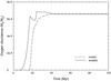 |
Fig. C.1 Evolution with time of the mass fraction of oxygen as derived from the analytical expression Eq. (C.3) (solid line) and from our numerical simulation (dashed line). See text for more detail. |
It is still possible to use the Eulerian form for the product  instead of just . We leave the exact derivation of the pertinent equations for a follow-up study.
should depend on because small stellar populations, characterized by a small amount of massive stars, could have an IMF truncated at relatively low masses (Ploeckinger et al. 2014). We neglect this effect in this paper.
Strictly speaking, this is only true when τc>τff. Otherwise, the density exponent should be set to 1.0.
In a more accurate approach, Λh can be directly calculated using Eq. (41).
For a more detailed analysis of these star formation criteria, see Vorobyov et al. (2012).
The total gas and DM masses are comparable in the inner several kpc.
Acknowledgments
This project was partly supported by the Russian Ministry of Education and Science Grant 3.961.2014/K and a Lise Meitner Fellowship, project number M 1255-N16 and RFBR Grant 15-01-00508. The simulations were performed on the Vienna Scientific Cluster (VSC-2). This publication is supported by the Austrian Science Fund (FWF). We are thankful to the anonymous referee for a very insightful review that helped improve the manuscript.
References
- Bakes, E. L. O., & Tielens, A. G. G. M. 1994, ApJ, 427, 882 [Google Scholar]
- Black, D. C., & Bodenheimer, P. 1975, ApJ, 199, 619 [NASA ADS] [CrossRef] [Google Scholar]
- Blondin, J. M., & Lufkin, E. A. 1993, ApJS, 88, 589 [NASA ADS] [CrossRef] [Google Scholar]
- Böhringer, H., & Hensler, G. 1989, A&A, 215, 147 [Google Scholar]
- Burkert, A., & Hensler, G. 1988, A&A, 199, 131 [Google Scholar]
- Brook, C. B., Stinson, G., Gibson, B. K., Wadsley, J., & Quinn, T. 2012, MNRAS, 424, 1275 [NASA ADS] [CrossRef] [Google Scholar]
- Clarke, D. A. 2010, ApJS, 187, 119 [NASA ADS] [CrossRef] [Google Scholar]
- Colella, P., & Woodward, P. R. 1984, J. Comput. Phys., 54, 174 [NASA ADS] [CrossRef] [MathSciNet] [Google Scholar]
- Creasey, P., Theuns, T., & Bower, R. G. 2013, MNRAS, 429, 1922 [NASA ADS] [CrossRef] [Google Scholar]
- Dalgarno, A., & McCray, R. A. 1972, ARA&A, 10, 375 [NASA ADS] [CrossRef] [Google Scholar]
- Dal la Vecchia, C., & Schaye, J. 2012, MNRAS, 426, 130 [Google Scholar]
- Famaey, B., & McGaugh, S. S. 2012, Liv. Rev. Relat., 15, 10 [Google Scholar]
- Famaey, B., & McGaugh, S. 2013, J. Phys. Conf. Ser., 437, 012001 [NASA ADS] [CrossRef] [Google Scholar]
- Genel, S., Vogelsberger, M., Springel, V., et al. 2014, MNRAS, 445, 175 [Google Scholar]
- Governato, F., Brook, C., Mayer, L., et al. 2010, Nature, 463, 203 [NASA ADS] [CrossRef] [PubMed] [Google Scholar]
- Hensler, G., & Recchi, S. 2010, IAU Symp., 265, 325 [NASA ADS] [Google Scholar]
- Hollenbach, D., & McKee, C. F. 1989, ApJ, 342, 306 [NASA ADS] [CrossRef] [Google Scholar]
- Hopkins, P. F., Narayanan, D., & Murray, N. 2013, MNRAS, 432, 2647 [NASA ADS] [CrossRef] [Google Scholar]
- Hunter, C. 1962, ApJ, 136, 594 [NASA ADS] [CrossRef] [Google Scholar]
- Jackson, J. P. 1975, Classical Electrodynamics (New York: Wiley) [Google Scholar]
- Katz, N. 1992, ApJ, 391, 502 [NASA ADS] [CrossRef] [Google Scholar]
- Kay, S. T., Pearce, F. R., Frenk, C. S., & Jenkins, A. 2002, MNRAS, 330, 113 [NASA ADS] [CrossRef] [Google Scholar]
- Kennicutt, R. C. 1998, ApJ, 498, 541 [NASA ADS] [CrossRef] [Google Scholar]
- Koeppen, J., Theis, C., & Hensler, G. 1995, A&A, 296, 99 [Google Scholar]
- Kroupa, P. 2001, MNRAS, 322, 231 [NASA ADS] [CrossRef] [Google Scholar]
- Kroupa, P. 2012, PASA, 29, 395 [NASA ADS] [CrossRef] [Google Scholar]
- Kulikov, I. 2014, ApJS., 214, 12 [NASA ADS] [CrossRef] [Google Scholar]
- Lasker, B. M. 1967, ApJ, 149, 23 [NASA ADS] [CrossRef] [Google Scholar]
- Leitherer, C., Schaerer, D., Goldader, J. D., et al. 1999, ApJS, 123, 3 [NASA ADS] [CrossRef] [Google Scholar]
- Lisenfeld, U., & Ferrara, A. 1998, ApJ, 496, 145 [NASA ADS] [CrossRef] [Google Scholar]
- Mac Low, M.-M., & Ferrara, A. 1999, ApJ, 513, 142 [NASA ADS] [CrossRef] [Google Scholar]
- Matteucci, F. 2001, The chemical evolution of the Milky Way (Dordrecht: Kluwer Academic Publishers), Astrophys. Space Sc. Lib., 253 [Google Scholar]
- Matteucci, F., & Recchi, S. 2011, ApJ, 558, 351 [Google Scholar]
- Melioli, C., & de Gouveia Dal Pino, E. M. 2004, A&A, 424, 817 [NASA ADS] [CrossRef] [EDP Sciences] [Google Scholar]
- Minchev, I., Chiappini, C., & Martig, M. 2013, A&A, 558, A9 [NASA ADS] [CrossRef] [EDP Sciences] [Google Scholar]
- Mitchell, N., Vorobyov, E. I., & Hensler, G. 2013, MNRAS, 428, 2764 [Google Scholar]
- Nomoto, K., Thielemann, F.-K., & Yokoi, K. 1984, ApJ, 286, 644 [Google Scholar]
- Norman, M. L., Wilson, J. R., & Barton, R. T. 1980, ApJ, 239, 968 [NASA ADS] [CrossRef] [Google Scholar]
- Ostriker, J. P., & Mark, J. W.-K. 1968, ApJ, 151, 1075 [NASA ADS] [CrossRef] [Google Scholar]
- Padovani, P., & Matteucci, F. 1993, ApJ, 416, 26 [NASA ADS] [CrossRef] [Google Scholar]
- Perret, V., Renaud, F., Epinat, B., et al. 2014, A&A, 562, A1 [NASA ADS] [CrossRef] [EDP Sciences] [Google Scholar]
- Pilkington, K., Gibson, B. K., Calura, F., et al. 2011, MNRAS, 417, 2891 [NASA ADS] [CrossRef] [Google Scholar]
- Ploeckinger, S., Hensler, G., Recchi, S., Mitchell, N., & Kroupa, P. 2014, MNRAS, 437, 3980 [NASA ADS] [CrossRef] [Google Scholar]
- Polyachenko, V. L., Polyachenko, E. V., & Strelnikov, A. V. 1997, Astron. Z., 23, 551 (translated Astron. Lett. 23, 483) [Google Scholar]
- Recchi, S. 2014, Adv. Astron., 2014 [Google Scholar]
- Recchi, S., & Hensler, G. 2013, A&A, 551, A41 [NASA ADS] [CrossRef] [EDP Sciences] [Google Scholar]
- Recchi, S., Matteucci, F., D’Ercole, A. 2001, MNRAS, 322, 800 [NASA ADS] [CrossRef] [Google Scholar]
- Recchi, S., Theis, C., Kroupa, P., & Hensler, G. 2007, A&A, 470, L5 [NASA ADS] [CrossRef] [EDP Sciences] [Google Scholar]
- Recchi, S., Calura, F., & Kroupa, P. 2009, A&A, 499, 711 [NASA ADS] [CrossRef] [EDP Sciences] [Google Scholar]
- Renaud, F., Bournaud, F., Emsellem, E., et al. 2013, MNRAS, 436, 1836 [NASA ADS] [CrossRef] [Google Scholar]
- Richtmyer, R. D., & Morton, K. W. 1995, Difference Methods for Initial Value Problems (New York: Wiley) [Google Scholar]
- Robitaille, T. P., & Whitney, B. A. 2010, ApJ, 710, 11 [Google Scholar]
- Roškar, R., Debattista, V. P., & Loebman, S. R. 2013, MNRAS, 433, 976 [NASA ADS] [CrossRef] [Google Scholar]
- Samland, M., Hensler, G., & Theis, Ch. 1997, 476, 544 [Google Scholar]
- Schaye, J., Crain, R. A., Bower, R. G., et al. 2015, MNRAS, 446, 521 [Google Scholar]
- Schure, K. M., Kostenko, D., Kaastra, J. S., Keppens, R., & Vink, J. 2009, A&A, 508, 751 [NASA ADS] [CrossRef] [EDP Sciences] [Google Scholar]
- Sedov, L. I., 1959, Similarity and Dimensional Methods in Mechanics (New York: Academic Press) [Google Scholar]
- Silich, S. A., & Tenorio-Tagle, G. 1998, MNRAS, 299, 249 [NASA ADS] [CrossRef] [Google Scholar]
- Silich, S., & Tenoreo-Tagle, G. 2001, ApJ, 552, 91 [NASA ADS] [CrossRef] [Google Scholar]
- Slyz, A. D. 2007, EAS Publ. Ser., 24, 89 [CrossRef] [EDP Sciences] [Google Scholar]
- Springel, V., & Hernquist, L. 2003, MNRAS, 339, 289 [Google Scholar]
- Stinson, G., Seth, A., Katz, N., et al. 2006, MNRAS, 373, 1074 [NASA ADS] [CrossRef] [Google Scholar]
- Stinson, G. S., Bovy, J., Rix, H.-W., et al. 2013, MNRAS, 436, 625 [NASA ADS] [CrossRef] [Google Scholar]
- Stone, J. M., & Norman, M. L. 1992, ApJSS, 80, 753 [NASA ADS] [CrossRef] [Google Scholar]
- Stone, J. M., & Norman, M. L. 1993, ApJ, 413, 198 [NASA ADS] [CrossRef] [Google Scholar]
- Tasker, E. J. et al. 2008, MNRAS, 390, 1267 [NASA ADS] [CrossRef] [Google Scholar]
- Teyssier, R., Pontzen, A., Dubois, Y., & Read, J. I. 2013, MNRAS, 429, 3068 [NASA ADS] [CrossRef] [Google Scholar]
- Theis, Ch., Burkert, A., & Hensler, G. 1992, A&A, 265, 465 [NASA ADS] [Google Scholar]
- Thornton, K., Gaudlitz, M., Janka, H.-T., & Steinmetz, M. 1998, ApJ, 500, 95 [NASA ADS] [CrossRef] [Google Scholar]
- Tinsley, B. M. 1980, Fundam. Cosm. Phys., 5, 287 [Google Scholar]
- Truelove, J. K., Klein, R. I., McKee, C. F., et al. 1997, ApJ, 489, L179 [NASA ADS] [CrossRef] [Google Scholar]
- Tomisaka, K., & Ikeuchi, S. 1988, ApJ, 330, 695 [NASA ADS] [CrossRef] [Google Scholar]
- Toomre, A. 1964, ApJ, 139, 1217 [NASA ADS] [CrossRef] [Google Scholar]
- Truelove, K. J., Klein, R. I., McKee, C. F., et al. 1998, ApJ, 495, 821 [NASA ADS] [CrossRef] [Google Scholar]
- Van Dishoeck, E. F., & Black, J. H. 1986, ApJSS, 62, 109 [NASA ADS] [CrossRef] [Google Scholar]
- van den Hoek, L. B., & Groenewegen, M. A. T. 1997, A&AS, 123, 305 [NASA ADS] [CrossRef] [EDP Sciences] [Google Scholar]
- Vázquez, G. A., & Leitherer, C. 2005, ApJ, 621, 695 [NASA ADS] [CrossRef] [Google Scholar]
- Vieser, W., & Hensler, G. 2007, A&A, 472, 141 [NASA ADS] [CrossRef] [EDP Sciences] [Google Scholar]
- Vogelsberger, M., Genel, S., Springel, V., et al. 2014, Nature, 509, 177 [NASA ADS] [CrossRef] [Google Scholar]
- von Neumann, J., & Richtmyer, R. D. 1950, J. Appl. Phys., 21, 232 [NASA ADS] [CrossRef] [MathSciNet] [Google Scholar]
- Vorobyov, E. I., & Basu, S. 2005, A&A, 431, 451 [NASA ADS] [CrossRef] [EDP Sciences] [Google Scholar]
- Vorobyov, E. I., & Theis, Ch. 2006, MNRAS, 373, 194 [NASA ADS] [CrossRef] [Google Scholar]
- Vorobyov, E. I., & Theis, Ch. 2008, MNRAS, 383, 817 [NASA ADS] [CrossRef] [Google Scholar]
- Vorobyov, E. I., Recchi, S., & Hensler, G. 2012, A&A, 543, A129 [NASA ADS] [CrossRef] [EDP Sciences] [Google Scholar]
- Vshivkov, V. A., Lazareva, G. G., Snytnikov, A. V., Kulikov, I. M., & Tutukov, A. V. 2011, ApJS, 194, 47 [NASA ADS] [CrossRef] [Google Scholar]
- Woosley, S. E., & Weaver, T. A. 1995, ApJS, 101, 181 [NASA ADS] [CrossRef] [Google Scholar]
- Zemp, M., Gnedin, O. Y., Gnedin, N. Y., & Kravtsov, A. V. 2012, ApJ, 748, 54 [NASA ADS] [CrossRef] [Google Scholar]
All Tables
All Figures
|
Fig. 1 Star volume density (left) and mean stellar age (right) as a function of time during the gravitational collapse of a stellar sphere of unit radius. The elapsed time is indicated in the left panel. Star formation is turned off for this test problem. The dash-dot-dotted lines shows the mean stellar age when calculated using the Eulerian form to account for bulk motions of stars instead of the Lagrangian form (see text for more detail). |
| In the text | |
|
Fig. 2 Cooling efficiency of gas as a function of temperature for the ionization fraction fion = 1.0 but varying metallicity (left panel) and for the gas with solar metallicity but varying ionization fractions fion (right column). |
| In the text | |
|
Fig. 3 Initial radial profiles of the gas surface density Σg (right) and Toomre Q-parameters (left) in models with different rotational support against gravity as indicated by the α-parameter. The horizontal dotted lines define the critical values of Q-parameter below which star formation is supposed to occur (see the text for more details). |
| In the text | |
|
Fig. 4 Gas density distribution of three model galaxies differing for the amount of rotational support: the α = 0.25 model 1 (left column), the α = 0.5 model 2 (middle column), and the α = 0.9 model 3 (right column). The time passed from the beginning of numerical simulations is indicated in the leftmost image of each row. The density scale (in cm-3) is shown in the upper strip. |
| In the text | |
|
Fig. 5 Gas surface density as a function of radius for the same models and at the same moments in time as in Fig. 4. In the upper panels, the initial density distribution is also indicated (dashed lines). The dotted lines in the middle column also show the distribution for the α = 0.5 model without stellar motion (see Sect. 5.2). |
| In the text | |
|
Fig. 6 Fraction of ejected gas mass as a function of time for the models with different values of α. The dashed double-dotted line refers to a model in which the stellar motion has been artificially suppressed (see Sect. 5.2). |
| In the text | |
|
Fig. 7 Star formation rates vs. time in three models differing in the value of the centrifugal support α. |
| In the text | |
|
Fig. 8 Similar to Fig. 4, but now for the stellar volume density distribution. The scale bar is in M⊙ pc-3. The right-hand column only presents the massive stars. |
| In the text | |
|
Fig. 9 Time evolution of the gas volume density in three models with α = 0.5. The l.h.s. column presents the time evolution in model 2, already shown in Fig. 4. The middle column shows model 4, in which the motions of stars are artificially suppressed. In the r.h.s. column we show model 5, for which the initial equilibrium distribution was constructed without taking gas self-gravity into account. Note the different evolutionary times in the latter model. |
| In the text | |
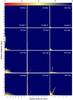 |
Fig. 10 Similar to Fig. 9, except for stellar volume density distribution. |
| In the text | |
|
Fig. A.1 Sod shock tube problem for the gas density (upper-left), velocity (upper-right), pressure (lower-left), and specific internal energy (lower-right). The numerical solution is shown by open circles, while the analytical one is plotted by solid lines. |
| In the text | |
|
Fig. A.2 Sedov point explosion test for the explosion energy 1051 erg and background density n = 0.01 cm-3. The analytic solution is shown by the red lines, while the numerical solutions along the z-axis, r-axis, and diagonal z = r are shown by the black, pink, and blue lines, respectively. The top left panel presents the solution for the tensor artificial viscosity with C2 = 6 ; the top right panel, for the scalar artificial viscosity and C2 = 3; the bottom left panel, for the tensor artificial viscosity and C2 = 3; and the bottom right panel, for the tensor artificial viscosity with off-diagonal terms set to zero and C2 = 6. |
| In the text | |
|
Fig. A.3 Sedov point explosion test for various explosion energies, background densities, and numerical resolutions as indicated in each panel. The tensor artificial viscosity with C2 = 6 is used for every plot. The line meaning is the same as in Fig. A.2. |
| In the text | |
|
Fig. A.4 Collapse of a pressure-free sphere showing the gas density at 0.985 that of the free-fall time. The left and right panels show the test results with and without the volume averaging corrections as described in Blondin & Lufkin (1993). The line meaning is the same as in Fig. A.2. |
| In the text | |
|
Fig. A.5 Specific angular momentum spectrum M(K), calculated using Eq. (A.1), for a collapsing sphere at 1.03tff. The analytic spectrum is shown with the solid line, while the test results are plotted with open circles. |
| In the text | |
|
Fig. A.6 Development of the KHI at different moments in time (see text for more detail). |
| In the text | |
|
Fig. A.7 Shock position versus time of a one-dimensional radiative shock during overstable oscillations. The shock positions for the flow velocities of 120 km s-1, 130 km s-1, and 150 km s-1 are plotted with solid, dash-dotted, and dotted lines, respectively. |
| In the text | |
|
Fig. B.1 Sod shock-tube problem for the stellar density (upper-left), velocity (upper-right), z-component of the stress tensor (lower-left), and square of the z-velocity dispersion (lower-right). The numerical solution is shown by open circles, while the analytical solution is plotted by solid lines. |
| In the text | |
|
Fig. C.1 Evolution with time of the mass fraction of oxygen as derived from the analytical expression Eq. (C.3) (solid line) and from our numerical simulation (dashed line). See text for more detail. |
| In the text | |
Current usage metrics show cumulative count of Article Views (full-text article views including HTML views, PDF and ePub downloads, according to the available data) and Abstracts Views on Vision4Press platform.
Data correspond to usage on the plateform after 2015. The current usage metrics is available 48-96 hours after online publication and is updated daily on week days.
Initial download of the metrics may take a while.