| Issue |
A&A
Volume 578, June 2015
|
|
|---|---|---|
| Article Number | A44 | |
| Number of page(s) | 11 | |
| Section | Numerical methods and codes | |
| DOI | https://doi.org/10.1051/0004-6361/201425204 | |
| Published online | 01 June 2015 | |
Testing for foreground residuals in the Planck foreground cleaned maps: A new method for designing confidence masks⋆
Institute of Theoretical Astrophysics, University of Oslo,
PO Box 1029 Blindern,
0315
Oslo,
Norway
e-mail:
This email address is being protected from spambots. You need JavaScript enabled to view it.
Received: 23 October 2014
Accepted: 19 February 2015
Abstract
We test for foreground residuals in the foreground-cleaned Planck cosmic microwave background (CMB) maps outside and inside the U73 mask commonly used for cosmological analysis. The aim of this paper is to introduce a new method of validating masks by looking at the differences in cleaned maps obtained by different component-separation methods. By analyzing the power spectrum, as well as the mean, rms, and skewness of needlet coefficients on separate equatorial bands running from the poles to the equator outside and inside the U73 mask, we first confirm that the pixels already masked by U73 are highly contaminated and cannot be used for cosmological analysis. We further find that the U73 mask needs extension in order to reduce large-scale foreground residuals to a level of less than 20% of the standard deviation of CMB fluctuations within the bands closest to the galactic equator. We also find 276 point-like residuals in the cleaned foreground maps that are currently not masked by the U73 mask. About 80 of these are identified as sz clusters that have not been properly subtracted by the component separation methods, and the rest are strongly correlated with the Planck dust map, indicating point-like dust residuals. Our final publicly available extended mask leaves 65.9% of the sky for cosmological analysis. This extended mask may be important for analyses on local sky patches; for the full sky power spectrum, we have shown that the unmasked residuals have very little impact.
Key words: cosmic background radiation / cosmology: observations / methods: numerical
The final extended mask (FITS format) is only available at the CDS via anonymous ftp to cdsarc.u-strasbg.fr (130.79.128.5) or via http://cdsarc.u-strasbg.fr/viz-bin/qcat?J/A+A/578/A44 and at http://folk.uio.no/frodekh/PS_catalogue/planck_extended_mask.fits
© ESO, 2015
1. Introduction
The recent results from ESA’s Planck (Planck Collaboration I 2014; Planck Collaboration I 2015) experiment have significantly improved cosmological parameter estimates, and today testable models that are able to describe many of the processes that have formed our universe are available. A plethora of phenomena are explained by the best-fit ΛCDM model, which complies with the cosmological principles of homogeneity and isotropy. For over a decade it has withstood serious challenges brought forth by comparison with high-precision data delivered by the WMAP satellite (Bennett et al. 2003, 2013; Hinshaw et al. 2007, 2009; Jarosik et al. 2011), not to mention other numerous experiments, such as BOOMERanG (de Bernardis et al. 2002), MAXIMA (Lee et al. 2001), DASI (Halverson et al. 2002), ACBAR (Kuo et al. 2007), and others.
In any cosmological analysis, it is imperative that the analyzed data be free of systematics. The most significant distortion of the underlying cosmological signal at GHz frequencies comes from foreground signals from our own galaxy in the form of synchrotron, free-free, and dust radiation, among others. In addition there are other galactic, as well as extra-galactic, foreground signals. The importance of foreground characterization has been well known for decades, and quite recently, the fidelity of the BICEP2 (Ade et al. 2014) B-mode results have been debated (see Flauger et al. 2014; Planck Collaboration Int. XXX 2015) due to uncertainties in the level of foreground contamination.
It seems that the most intriguing discrepancies between observed CMB data and the best-fit model occurs at the very largest angular scales. The so-called hemispherical power asymmetry first reported by Eriksen et al. (2004) and Hansen et al. (2004), and subsequently re-analyzed in a number of papers (see e.g. Hansen et al. 2009) and also observed in Planck (Planck Collaboration XXIII 2014), has been shown to be statistically significant at least at the 3.3σ level. This curious effect persists in several experiments and argues against an explanation in terms of systematic effects, and it may pose a challenge to the standard model.
It is of utmost importance that any cosmological analysis is performed on maps where foreground contaminations are at a minimum; as a result, consistency checks should always be performed whenever possible. In this paper, we aim to shine a bright light on the publicly available Planck data maps and especially to examine the level of any residuals, if there are any. Foregrounds were subtracted from Planck raw data using four separate cleaning algorithms: SMICA (spectral matching independent component analysis; Delabrouille et al. 2003), NILC (needlet internal linear combination; Remazeilles et al. 2011), SEVEM (spectral expectation via maximization-expectation; Martínez-González et al. 2003), and Commander-Ruler (Eriksen et al. 2008). Common to all methods is the use of observations at multiple frequencies in order to reduce foregrounds. The SMICA method has been dubbed the main product in the first release.
The SMICA method consists of three basic steps. In the first step, spectral statistics are derived from a matrix computed from correlations between observations in harmonic space, where each observation is assumed to be a superposition of individual components. Subsequently, a component model is fitted to the result, which is then used to estimate a Wiener filter in harmonic space. The filtered spectral components are then transformed back into pixel space using the inverse spherical harmonic transform.
The SEVEM method treats all components, except the CMB signal, as generalized noise. Internal templates (Hansen et al. 2006) are fitted and subtracted from the frequency maps.
The NILC is a generalization of the WMAP ILC method, which constructs multi-dimensional filters that are used to estimate the emission from complex components, which are spawned by multiple correlated emissions. From a given map, which can be thought of as a superposition of components, the CMB is thus removed, as opposed to the usual procedure of removing the non-cosmological signals. It is generalized, in the sense that the number of foreground components is not assumed fixed. The method performs local estimation of the foregrounds, in order to suppress the instrumental noise levels.
The Commander-Ruler method (henceforth referred to as CR) implements Bayesian component separation in pixel space, fitting a parametric model to the data by sampling the posterior distribution. Gibbs sampling is used to fit foreground amplitude and spectral parameters at low resolution (typically Nside = 256), and the amplitudes are subsequently converted to high resolution by solving a least squares system of equations in each pixel, with the spectral parameters fixed to their values from the low-resolution run, while at the same time taking pixelization effects into account in order to avoid sharp boundaries in the high-resolution map.
In the first Planck release, each method provided its own mask based on the properties of each cleaned CMB map. The available sky fraction in these masks varies from 75% to 93%. In most cosmological analyses, the so-called U73 mask, the product of all these individual masks, is applied. The aim of this paper is to investigate (1) if the cleaned maps are sufficiently clean outside the U73 mask and (2) if some areas of the sky inside the masked pixels of the U73 maps are safe for cosmological analysis. Both the galactic mask and the point source mask are investigated. To assess these questions, we (1) study the local power spectra around the galactic plane; (2) study the mean, rms, and skewness of needlet coefficients in bands around the U73 cut, both in the fully foreground separated maps and in the difference maps between the different methods; and (3) investigate the presence of residual unmasked point sources in the difference maps based on the approach described in Scodeller et al. (2012a).
A large part of the analysis undertaken in this paper is based on needlets. Their localization properties both in pixel and harmonic space make them particularly suited to locating foreground residuals. Wavelets (and in particular needlets) have previously been applied to several aspects of statistical CMB analysis, such as tests for non-Gaussianity and asymmetries (Vielva et al. 2004; Cabella et al. 2004; Wiaux et al. 2006, 2008; McEwen et al. 2008; Marinucci et al. 2008; Pietrobon et al. 2008; Rudjord et al. 2009), polarization analysis (Cabella et al. 2007), foreground component separation and reduction (Hansen et al. 2006), point source detection in CMB data (Cayón et al. 2000; González-Nuevo et al. 2006; López-Caniego et al. 2007; Massardi et al. 2009; Scodeller et al. 2012b), and power spectrum estimation (Basak & Delabrouille 2012). Also, the cold spot was first detected through wavelet analysis (Cruz et al. 2005). For a general introduction to needlets and their properties, see e.g. (Baldi et al. 2009; Marinucci & Peccati 2011).
The approach which we develop and apply to Planck temperature data in this paper is a methodology which allows the construction of a common mask based on data cleaned with many different methods. We show the importance of applying such a procedure in order to obtain a consistency test of component separation methods as well as in designing a fiducial mask. For the coming release of Planck polarization data where the foreground properties are less known, such an approach may become even more important.
In Sect. 2 we discuss the data products used in this paper. In Sect. 3 we discuss the details of our methodology and define several tests applied to the cleaned maps. In Sect. 4 we analyze individual maps, whereas in Sect. 5 the analysis is repeated, but this time on difference maps in order to perform consistency checks. In Sect. 6 we use difference maps in needlet space to manipulate the mask in order to explore how statistics is affected by either adding, or subtracting, parts of the sky close to the galactic plane. The point source mask is investigated in Sect. 7 and we discuss our findings in Sect. 8.
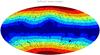 |
Fig. 1 Seven-band masks on which the analysis is performed. A single band mask consists of a set of pixels on both the northern and southern galactic hemispheres as indicated by the matching color schemes. |
2. Data
In this paper we use the publicly available NILC, SMICA, SEVEM, and CR foreground cleaned maps as well as their beam functions and accompanying FFP6 simulation sets. The sixth round full focal plane (FFP6) simulations have been passed through the component separation pipeline and therfore have beam and noise properties similar to the foreground cleaned maps. The method specific masks are used, along with the common mask based on their product. We also create jack-knife maps based on the difference between half-ring maps of the data. The advantage of jack-knife maps is that they have noise properties very close to the noise properties of the actual data. As described in detail below, they are used to adjust the noise level in the simulations, in order to obtain best possible agreement with the noise properties in the data.
3. Method
To study the variation in possible foreground residuals with distance from the galactic plane, we constructed seven bands in each hemisphere starting from the borders of the U73 mask and proceeding out towards the polar caps. We number these bands from 1 to 7, each “band” consists of the sum of the corresponding bands in both hemispheres. The northern and southern bands are combined to increase statistics. Band 1 consists of the two bands closest to the U73 mask, band 7 consists of the polar caps (see Fig. 1). The bands are constructed by smoothing the U73 mask with a large beam, then including all pixels below a certain threshold. This process is repeated for each band. The sky fractions covered by bands 1 to 7 are 0.145, 0.138, 0.126, 0.11, 0.096, 0.078 and 0.041 respectively. A further division of the first bands will be necessary as detailed below.
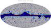 |
Fig. 2 Constructed bands in the interior of the U73 mask, prior to data reduction. |
Furthermore, using the same approach as described above to construct bands outside U73, we also constructed five bands inside the U73 mask. This in order to test whether some of these areas appear sufficiently clean for cosmological analysis. In Fig. 2 we show these inside bands. The LFI and HFI Planck point source masks (Planck Collaboration XXVIII 2014) are used to ensure that no pixels in the inside bands are contaminated by point sources.
We estimate a set of quantities in each of these bands and compared them to the corresponding quantities within the same band on simulated maps. The indicators of foreground residuals that are used are the following:
-
1.
We estimate the power spectrum within each band using theMASTER approach (Hivonet al. 2002). Due to the small skyfraction available to each band, we bin the resulting spectra in binsof 10 multipoles.
-
2.
We calculate the mean, rms, and skewness of needlet coefficients for each band. In this process each needlet coefficient is weighted by the inverse of its CMB+noise variance. We use standard needlets with needlet base B = 1.8393 and scales j = [ 2,11 ] which correspond to multipoles in the range ℓ = [ 2,1500 ].
These indicators are calculated on two sets of maps:
-
1.
The officially released SMICA, SEVEM, NILC, andCR cleaned Planck maps.
-
2.
On difference maps between pairs of cleaned maps. For each difference map, we smooth the maps to a common resolution and subtract. In the difference maps, the CMB cancels out and only noise as well as differences in foreground residuals are present. We found that the noise properties of the data difference maps deviate significantly from the simulated difference maps. We used the jack-knife difference maps for the data to fit and adjust an amplitude correction factor to the noise levels in the simulated maps, scale by scale and band by band (although the variation with band is very small). After this correction we found a very good agreement between the noise level in the simulated maps and in the jack-knife maps. The correction factors for some difference maps are shown in Fig. 3.
We further applied the approach in Scodeller et al. (2012a) to amplify point sources in the difference maps. This approach together with the results will be discussed in greater detail in Sect. 7.
We assess significance of our results by studying deviations by plots of (x − ⟨ x ⟩ ) /σ where x is any of the aforementioned indicators, ⟨ x ⟩ and σ are their corresponding mean and standard deviation from simulations.
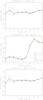 |
Fig. 3 Bias correction factors in each band outside the U73 mask for selected difference maps, see Fig. 1. Top: correction factors in pixel space for SEVEM-NILC. Middle: correction factors for NILC-SMICA. Bottom: correction factors applied to SMICA-SEVEM. |
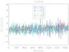 |
Fig. 4 (Cℓ − ⟨ Cℓ ⟩ ) /σℓ obtained from the SEVEM map. The data have been binned in Δℓ = 10 sized bins in order to avoid singular matrices. The legend label “BX” refers to band number “X”, as defined above. The corresponding plots for the other methods are very similar and not shown. |
4. Single map analysis
In this section we present the results for each individual foreground cleaned map. These maps have both CMB and noise present, although the noise is sub-dominant on most scales. In Figs. 4–6 we show results on the power spectrum as well as needlet mean, rms, and skewness, band by band and scale by scale. While Fig. 5 shows the results as a function of needlet scale, Fig. 6 shows the same but as a function of band on the x-axis. The purpose of the former is to show the scale dependence, the purpose of the latter is to show whether there is an increase towards band 1 (galactic plane) which could indicate foreground residuals.
We find very good agreement between data and simulations, although from Fig. 5 one can clearly see, in particular for the rms of the needlet coefficients, the effect of unresolved point sources on small scales (high j). This effect is seen even clearer in the difference maps presented in the next section. We can see that this effect is not as pronounced in the SEVEM maps as in the other maps where the increase in rms with scale is not seen in the very last scale. This could indicate that SEVEM does better in subtracting point sources than the other methods. Another possible explanation here is that the residual noise mismatch between data and simulations affects the rms in the last scale. Note also that the unresolved point sources are not seen in skewness. This is expected given the very low skewness signal expected from unresolved point sources in the cleaned maps.
Note also that both the mean and skewness of band 2 appears systematically below zero over most scales. In the simulated data we found that in 30% of the cases, the mean lies below zero on all scales in at least one band. For skewness this occurred in 12% of the simulations. Therefore we conclude that the behavior of band 2 can be well explained as a statistical fluctuation. Note further in Fig. 6 that for the three largest scales there is a clear increase towards the galactic plane in all methods. This is particularly seen in bands 1−3, the ones closest to the galactic equator. This is only seen in the rms of the needlet coefficients. The rms can only increase with foregrounds (while the mean and skewness can increase or decrease), as foreground residuals would generally not subtract power from the map. This increase in rms towards the galactic plane, although the increase is towards the expected rms, can therefore be interpreted as an increasing level of foreground residuals. This is further supported by the fact that this increase disappears with an extended mask as we show later. We do not show mean and skewness in this figure as no signs of residuals were seen in those cases.
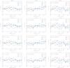 |
Fig. 5 (x − ⟨ x ⟩ ) /σ where x corresponds to mean (left column), rms (middle column), and skewness (right column) of needlet coefficients computed from SMICA, SEVEM, NILC, and CR maps. The various bands, B1 to B7 are shown in Fig. 1. |
5. Difference map analysis
In this section we analyze inter-method consistency of the component separation by looking at difference maps between six pairs of the four available foreground cleaned maps. These difference maps consist only of noise and differences in foreground residuals between the methods. Since the CMB has been eliminated the difference maps are much more sensitive to foreground residuals and we use these maps to quantify to which degree the foreground cleaned maps are reliable. Then in the next section we use these results in order to suggest an improved common mask.
Due to the higher sensitivity of the difference maps to foreground residuals, we find residuals in most bands and scales for most of the computed quantities. Knowledge of whether these residuals may bias cosmological results is of very high interest. We therefore plot (x − ⟨ x ⟩ ) /σCMB instead of (x − ⟨ x ⟩ ) /σ where σCMB is the standard deviation derived from maps with both CMB and noise in them. On the other hand σ is the expected noise standard deviation of the difference maps. In this way we measure the residuals in units of fraction of the standard deviation of CMB fluctuations. If the residuals are larger than 0.2σCMB it means that they may bias cosmological results by the order of 0.2σCMB. For needlet skewness the residuals are still small, so in this case we show (x − ⟨ x ⟩ ) /σ as previously.
 |
Fig. 6 Same as Fig. 5 for rms only but now plotted with the band number on the x-axis and with color codes indicating needlet scales. |
 |
Fig. 7 (Cℓ − ⟨ Cℓ ⟩ ) /σCMB for SEVEM-NILC, NILC-SMICA, SMICA-SEVEM, and SEVEM-CR derived from MASTER estimated power spectra. |
The results for the power spectrum are shown in Fig. 7, for the multipole interval ℓ ∈ [ 500,1500 ]. For values [ 0,500 ] the agreement between simulations and data is perfect, and hence not shown. We first consider the SMICA, NILC, and SEVEM maps: First note the general increase towards smaller scales from unresolved point sources visible in all bands. As we approach ℓ = 1500 we notice that the difference increases, especially for the difference maps including SEVEM. This increase is particularly large in the two bands close to the galactic plane where most foreground residuals are expected. The difference NILC-SMICA is generally much smaller than the differences including SEVEM suggesting residuals which are either present only in SEVEM or common for both NILC and SMICA (notice that the similarity between NILC and SMICA was also noted by the Planck team in Planck Collaboration XII 2014). In order to obtain further information, we continue with wavelet space analysis.
In Figs. 8 and 9 we show the results for the moments of the needlet coefficients. Looking at the rms measure for larger scales, one important observation is that while for SEVEM, NILC, and SMICA combinations, the residuals are <0.2σCMB for bands >2, SEVEM-CR (and all other CR combinations, not shown) have residuals >0.2σCMB for all bands. In fact, even when extending the mask as described in the next section, we are unable to improve results with CR combinations significantly. We conclude that the CR map has larger differences compared to the other three maps, than the other three maps have between themselves. We are therefore, as detailed in the next section, capable of creating an extended mask with improved results using SMICA, NILC, and SEVEM only. The CR map however is too different to allow for construction of a common mask which brings all four maps in full agreement. We therefore decided to exclude the CR map from the work in the next section.
However, we want to point out (1) the fact that while the CR map is different from the other three maps, these differences are still so tiny that they did not show up when single channel analysis including CMB was performed in the previous section. Furthermore (2) we cannot conclude from this that CR is the map with the highest foreground residuals. The approach used in the construction of the CR map takes better into account variation of foreground properties across the sky compared to the other three methods. It can therefore not be excluded that there are common residuals in the other three maps which give rise to the larger difference between CR and other methods.
In the following we will consider only combinations with SMICA, NILC, and SEVEM. Looking at the mean of needlet coefficients we find again that NILC and SMICA are very similar with differences <0.1σCMB for all bands, while SEVEM shows differences >0.1σCMB for band 1 (close to the galactic plane) compared to the other two maps.
We find that the rms measure is the measure most sensitive to foreground residuals. First of all the strong increase at the last 2−3 needlet scales due to unresolved point sources is now very visible. We observe that band 1 again shows strong deviation (>0.2σCMB) between methods, now also visible in the difference NILC-SMICA. The skewness measure also supports the fact that there are large differences between methods in band 1. Band 4 shows a very strong outlier in skewness only for the NILC-SMICA difference map. We have not been able to identify the source of this latter difference, however, with the new mask which is derived in the following sections, we find that the skewness outliers previously present on band 1 now disappear. Looking at Fig. 9 we can clearly see the increase towards the galactic plane for the large scales, in particular for bands 1 and 2. These results provide an incentive to further study the bands closest to the galactic center, bands 1 and 2. It is already clear from the inferences made so far, that these bands are not consistent between foreground reduction algorithms, however, we may not infer from the obtained data, which of the methods, if not all, have residuals causing these inconsistencies. The strategy now, is to examine the needlet coefficients belonging to difference maps SEVEM-NILC, NILC-SMICA, and SMICA-SEVEM and use these to construct a new confidence mask.
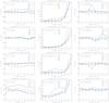 |
Fig. 8 (x − ⟨ x ⟩ ) /σ where x corresponds to mean (left column), rms (middle column) and skewness (right column) of needlet coefficients computed on SEVEM-NILC, NILC-SMICA, SMICA-SEVEM, and SEVEM-CR. Notice also that the standard deviation used in the skewness plots is the pure noise standard deviation while for mean and rms, the standard deviation is the one from CMB plus noise. The various bands, B1 to B7 are shown in Fig. 1. |
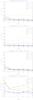 |
Fig. 9 Same as Fig. 8 for rms only but now plotted with the band number on the x-axis and with color codes indicating needlet scales. |
6. Improving the mask
The U73 mask is defined to be the union of all individual foreground method masks, meaning that if one of the method masks excludes a given pixel, then the combined mask excludes it as well, even if the other masks include it. One might contemplate if it can be made smaller, or given the results from the previous section, be extended. The current galactic mask, including masking of point sources, allows a fraction fsky = 73.7% of the sky to be used for cosmological analysis, deeming 26.3% of the sky improper. This stands in stark contrast to, for example, the SMICA mask which has an fsky ~ 88%. To our knowledge, no analysis using all three foreground method maps simultaneously has been done in order to construct a joint confidence mask. Such an analysis is the topic of this section.
Our methodology is to examine the needlet coefficients scale by scale in wavelet space. This will allow construction of “scale masks”, Mj(i), where j is the needlet scale, and i is a pixel index. The advantage we have over methods that use pixel maps is that we can examine each scale individually and thus be more flexible. From these masks we can then define the complete mask as the product of scale masks over all relevant scales: 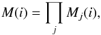 (1)where M(i) is the total mask for a given difference map and the product runs over all relevant scales j.
We obtain the scale mask for a given pixel i from the needlet coefficients of the difference map divided by their standard deviation obtained from simulations: 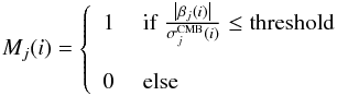 (2)where βj(i) is the needlet coefficent from a difference map and
  is the corresponding standard deviation including the expected standard deviation from CMB. We use difference maps for j ∈ [ 3,11 ]. In order to minimize the influence of foreground residuals, we require these to have values less than
  for j ≤ 7. For j> 7 the noise level is higher than in some pixels and we therefore use the maximum value in the jack-knife difference map as a threshold. For the pixels exceeding the threshold we zero all pixels within a disc with scale dependent radius ranging between 24° and 0.18° at j = 3 and j = 11 respectively. The disc radius is calculated according to the recommended procedure in Scodeller et al. (2012b). In this way we obtain a new and more conservative mask.
As it turns out that large regions of band 1 are removed in the extended mask, we found that these bands need a further subdivision into bands 1a, 1b and 1c, where band 1a lies closest to the galactic plane, and band 1c lies farthest away from it. We use these smaller bands to test the results with the extended mask close to the borders of the U73 mask. In Figs. 10 and 11 we show results on the rms of needlet coefficients from the analysis with the extended mask. Included in the plots are results from analysis on the first band inside the U73 mask, defined in Fig. 2, and labeled iB1. Pixels analyzed on the inside bands have undergone the same mask extension procedure, as the bands on the outside of U73. After this mask extension only a sky fraction of 2.2% of the original 4.1% remains in band iB1. Still, we clearly see from the figure that this band is unsuitable for cosmological analysis, the same conclusion is valid for all five inside bands. Note that in Fig. 10 we show the full band 1 and 2 analyzed with the U73 mask whereas bands 1a,b,c and iB1 were analysed with the extended mask. We find that band 1a has to be fully discarded in order to achieve residuals <0.2σCMB for the large scales whereas bands 1b and 1c can be kept with this new extended mask. From Fig. 11 we can see how the new extended mask has removed the increase in rms towards the galactic plane. In fact, only in band 1b are there signs of an increase, but it is well below <0.2σCMB. Also notice that band 2 has been subdivided into bands 2a and 2b, as done previously with band 1, in order to examine if band 2 may be fully used with the new mask. Band 2a lies closest to the galactic plane while band 2b lies farthest away. From the plots shown we conclude that entire band 2 may be kept.
We have thus arrived at a further extended mask which equals the mask obtained above but with the further extension that all pixels in band 1a are set to zero. This new mask gives satisfactory results for all measures used in this paper allowing fsky = 65.9% of the sky for cosmological analysis.
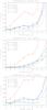 |
Fig. 10 From top: (x − ⟨ x ⟩ ) /σCMB for SEVEM-NILC, NILC-SMICA, and SMICA-SEVEM for rms after applying the extended mask. We show results on the full bands 1 and 2 using the old U73 mask. Band 1 has been divided into B1a, B1b, and B1c. We show results for these smaller bands as well as for the first band (iB1) inside the U73 mask after the mask extension described in the text has been applied. |
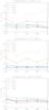 |
Fig. 11 Same as Fig. 10 but now plotted with the band number on the x-axis and with color codes indicating needlet scales. Band 2 has been divided into B2a and B2b. In this figure we only show results based on the new extended mask. |
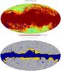 |
Fig. 12 Top: 276 new point source detections (overplotted on the Planck dust map) indicated by large discs for illustration, the actual holes are much smaller. The circles indicate sources indentified as sz clusters from the Planck sz catalogue, the full discs indicate sources which have not been identified in other catalogues but which seem to trace galactic dust emission. Bottom: new extended U66 mask (yellow) with the U73 mask (blue). |
7. Point source extensions
We have seen in the previous plots that unresolved point sources give rise to large discrepancies between the methods on smaller angular scales. We cannot do much to remove the unresolved sources, but we check if there are sources left in the difference maps which can be resolved and therefore masked.
We follow the approach of Scodeller et al. (2012a) to detect residual sources. The Scodeller method is based on detecting outliers in the needlet transformed maps. Here we use the difference between the foreground corrected maps, identifying needlet coefficients that exceed 5σ of what we would expect from noise alone. Once the excessive needlet coefficients are found, we perform a search in the nearby area to find the most likely centre of the point source, in our case we use the centre that gives us the highest fitted amplitude. We find that the needlet scales B = 1.5 and j = 17 give the largest increase in point source amplitudes.
We find 276 point sources at >5σ in the difference maps. These point sources include only those which are not already masked by the above described extended U73 mask. Many of these are common to several difference map combinations, others are detected only in one combination but is present but slightly below the detection limit in others. Comparing the position of these sources to the PCCS (Planck Collaboration XXVIII 2014), PLANCKSZ (Planck Collaboration XXIX 2014), GB6 (Gregory et al. 1996), NVSS (Condon et al. 2002), and SUMSS (Mauch et al. 2003) catalogues, we only found good fits to 80 sources in the PLANCKSZ catalogue. Due to the weak amplitude and slow spectral variation of sz (Sunyaez-Zeldovich) sources these are not easily removed in the component separation procedure. It is therefore not surprising to find many of these in the difference maps.
In the top panel of Fig. 12 we show the position of these sources on top of the Planck dust map. The full discs which have not been identified in source catalogues show a very strong correlation with the Planck dust map indicating an origin within our own galaxy. These are most probably knots of galactic cirrus which also plagued the point source detection procedure of the Planck team (Planck Collaboration XXVIII 2014).
We include point source holes with radius 0.1° for all these sources in our extended U73 mask (this is similar to the HFI point source holes used by the Planck team assuming the 5′ FWHM (Full Width Half Maximum) beam used for all frequencies >143 GHz). The final extended mask now has a usable sky fraction of 65.9%. In Fig. 12 (bottom) we show the final extended U66 mask which we have made publicly available1.
8. Conclusions
In this work, the SMICA, SEVEM, NILC, and CR foreground cleaned Planck data maps have been compared to simulated data. It is known that the current maps are recommended for joint cosmological analysis up to ℓmax = 1500, but for smaller scales, the complex foregrounds and noise properties of the maps are not yet fully understood. We have therefore limited our study to ℓ ≤ 1500.
The aim of this work was to test for foreground residuals in the cleaned maps outside and inside the U73 mask, checking whether the U73 mask needs extension or if it can be made smaller and still be suitable for cosmological analysis. We divided the sky outside U73 into seven bands north and south of the galactic equator and tested for foreground residuals in these bands by analyzing their local power spectra as well as mean, rms, and skewness of needlet coefficients at several scales. We performed this test, both on the individual foreground cleaned maps and on difference maps constructed from pairs of these maps. We found that in particular the rms of needlet coefficients on difference maps was highly sensitive to residuals.
Based on the needlet rms test, we found that all the difference maps where the CR foreground cleaned map was present, the differences to the other maps were so large that we decided to exclude the CR map from further analysis. Even with a highly extended mask we were unable to make the CR map agree with the other maps at a satisfactory level. Note that this difference was not seen in the full maps including CMB, only in the difference maps, and only at a level of 0.3 to 0.4 CMB standard deviations. This may influence some cosmological analyses, but is too small to significantly influence, for instance, the power spectrum. Note however that it is not clear whether this difference comes from large residuals in the CR map or in the other three maps.
The other three methods were found to agree with differences less than 20% of the standard deviation of the CMB over most scales after an extended U73 mask was applied. This extended U73 mask was constructed by removing pixels where the needlet coefficients were found to be higher than a certain scale dependent threshold. Analysis of bands inside the U73 mask revealed such high levels of foreground contamination that we can confirm that areas which are currently masked by U73 cannot be reliably used for cosmologial analysis. Our extended mask was finally further extended by point source holes for point sources detected in the difference maps. 276 point sources which are not masked in U73 were detected in the difference maps. Our final extended U66 mask, including point source holes for the additional sources has a usable sky fraction of 65.9% and is publicly available. We recommend the use of this mask rather than the U73 mask for cosmological analysis of the foreground cleaned Planck maps, in particular for analyses which are performed on smaller patches on the sky rather than on the full sky. On small fsky patches the relative fraction of contaminated area will be larger than compared to the full sky, and hence the impact of foreground residuals increases. As we did not detect these residuals in the individual foreground cleaned maps, only in the differences between these, we expect that their impact on CMB analyses using the full sky will be small.
We further note that the method presented here can easily be extended to polarization. We have seen that simply taking the product of the individual method specific masks does not necessarily yield a common mask which masks all residuals. By using the differences between the cleaned maps we can extend this simple common mask according to the desired acceptance level of foreground residuals. This may be of even higher importance for the soon-to-be-released Planck polarization maps as the properties of polarized foregrounds are much less known than for temperature.
The mask is available at the CDS and at F. K. Hansen‘s repository, see title page for url.
Acknowledgments
Maps and results have been derived using the Healpix2 software package developed by Gorski et al. (2005). This work was performed on the Abel Cluster, owned by the University of Oslo and the Norwegian metacenter for High Performance Computing (NOTUR), and operated by the Department for Research Computing at USIT, the University of Oslo IT-department, http://www.hpc.uio.no/. This work is based on observations obtained with Planck (http://esa.int/Planck), an ESA science mission with instruments and contributions directly funded by ESA Member States, NASA, and Canada. The development of Planck has been supported by: ESA; CNES and CNRS/INSU-IN2P3-INP (France); ASI, CNR, and INAF (Italy); NASA and DoE (USA); STFC and UKSA (UK); CSIC, MICINN and JA (Spain); Tekes, AoF and CSC (Finland); DLR and MPG (Germany); CSA (Canada); DTU Space (Denmark); SER/SSO (Switzerland); RCN (Norway); SFI (Ireland); FCT/MCTES (Portugal); and PRACE (EU). We acknowledge the use of the Planck Legacy Archive.
References
- Ade, P. A. R., Aikin, R. W., Barkats, D., et al. 2014, Phys. Rev. Lett., 112, 241101 [NASA ADS] [CrossRef] [PubMed] [Google Scholar]
- Baldi, P., Kerkyacharian, G., Marinucci, D., & Picard, D. 2009, Ann. Statistics, 37, 1150 [Google Scholar]
- Basak, S., & Delabrouille, J. 2012, MNRAS, 419, 1163 [NASA ADS] [CrossRef] [Google Scholar]
- Bennett, C. L., Halpern, M., Hinshaw, G., et al. 2003, ApJS., 148, 1 [NASA ADS] [CrossRef] [Google Scholar]
- Bennett, C. L., Larson, D., Weiland, J. L., et al. 2013, ApJS, 208, 20 [Google Scholar]
- Cabella, P., Hansen, F., Marinucci, D., Pagano, D., & Vittorio, N. 2004, Phys. Rev. D, 69, 063007 [NASA ADS] [CrossRef] [Google Scholar]
- Cabella, P., Natoli, P., & Silk, J. 2007, Phys. Rev. D, 76, 123014 [NASA ADS] [CrossRef] [Google Scholar]
- Cayón, L., Sanz, J. L., Barreiro, R. B., et al. 2000, MNRAS, 315, 757 [NASA ADS] [CrossRef] [Google Scholar]
- Condon, J. J., Cotton, W. D., Greisen, E. W., et al. 2002, VizieR Online Data Catalog, VIII/065 [Google Scholar]
- Cruz, M., Martínez-González, E., Vielva, P., & Cayón, L. 2005, MNRAS, 356, 29 [NASA ADS] [CrossRef] [Google Scholar]
- de Bernardis, P.Ade, P. A. R., Bock, J. J., et al. 2002, ApJ, 564, 559 [NASA ADS] [CrossRef] [Google Scholar]
- Delabrouille, J., Cardoso, J.-F., & Patanchon, G. 2003, MNRAS, 346, 1089 [NASA ADS] [CrossRef] [Google Scholar]
- Eriksen, H. K., Hansen, F. K., Banday, A. J., Górski, K. M., & Lilje, P. B. 2004, ApJ, 605, 14 [NASA ADS] [CrossRef] [Google Scholar]
- Eriksen, H. K., Jewell, J. B., Dickinson, C., et al. 2008, ApJ, 676, 10 [NASA ADS] [CrossRef] [Google Scholar]
- Flauger, R., Hill, J. C., & Spergel, D. N. 2014, JCAP, 08, 039 [NASA ADS] [CrossRef] [Google Scholar]
- González-Nuevo, J., Argüeso, F., López-Caniego, M., et al. 2006, MNRAS, 369, 1603 [NASA ADS] [CrossRef] [Google Scholar]
- Gorski, K. M., Hivon, E., Banday, A. J., et al. 2005, ApJ, 622, 759 [NASA ADS] [CrossRef] [Google Scholar]
- Gregory, P. C., Scott, W. K., Douglas, K., & Condon, J. J. 1996, ApJS, 103, 427 [NASA ADS] [CrossRef] [Google Scholar]
- Halverson, N. W., Leitch, E. M., Pryke, C., et al. 2002, ApJ, 568, 38 [NASA ADS] [CrossRef] [MathSciNet] [Google Scholar]
- Hansen, F. K., Banday, A. J., & Górski, K. M. 2004, MNRAS, 354, 641 [NASA ADS] [CrossRef] [Google Scholar]
- Hansen, F. K., Banday, A. J., Eriksen, H. K., Górski, K. M., & Lilje, P. B. 2006, ApJ, 648, 784 [Google Scholar]
- Hansen, F. K., Banday, A. J., Górski, K. M., Eriksen, H. K., & Lilje, P. B. 2009, ApJ, 704, 1448 [NASA ADS] [CrossRef] [Google Scholar]
- Hinshaw, G., Nolta, M. R., Bennett, C. L., et al. 2007, ApJS., 170, 288 [NASA ADS] [CrossRef] [Google Scholar]
- Hinshaw, G., Nolta, M. R., Bennett, C. L., et al. 2009, ApJS, 225 [NASA ADS] [CrossRef] [Google Scholar]
- Hivon, E., Górski, K. M., Netterfield, C. B., et al. 2002, ApJ, 567, 2 [NASA ADS] [CrossRef] [Google Scholar]
- Jarosik, N., Bennett, C. L., Dunkley, J., et al. 2011, ApJS, 192, 14 [NASA ADS] [CrossRef] [Google Scholar]
- Kuo, C. L., Ade, P. A. R., Bock, J. J., et al. 2007, ApJ, 664, 687 [NASA ADS] [CrossRef] [Google Scholar]
- Lee, A. T., Ade, P., Balbi, A., et al. 2001, ApJ, 561, L1 [NASA ADS] [CrossRef] [Google Scholar]
- López-Caniego, M., González-Nuevo, J., Herranz, D., et al. 2007, ApJS, 170, 108 [NASA ADS] [CrossRef] [Google Scholar]
- Marinucci, D., & Peccati, G. 2011, Random Fields on the Sphere (Cambridge University Press), Cambridge Books Online [Google Scholar]
- Marinucci, D., Pietrobon, D., Balbi, A., et al. 2008, MNRAS, 383, 539 [NASA ADS] [CrossRef] [Google Scholar]
- Martínez-González, E., Diego, J. M., Vielva, P., & Silk, J. 2003, MNRAS, 345, 1101 [NASA ADS] [CrossRef] [Google Scholar]
- Massardi, M., López-Caniego, M., González-Nuevo, J., et al. 2009, MNRAS, 392, 733 [NASA ADS] [CrossRef] [Google Scholar]
- Mauch, T., Murphy, T., Buttery, H. J., et al. 2003, MNRAS, 342, 1117 [NASA ADS] [CrossRef] [Google Scholar]
- McEwen, J. D., Hobson, M. P., Lasenby, A. N., & Mortlock, D. J. 2008, MNRAS, 388, 659 [NASA ADS] [CrossRef] [Google Scholar]
- Pietrobon, D., Amblard, A., Balbi, A., et al. 2008, Phys. Rev. D, 78, 103504 [NASA ADS] [CrossRef] [Google Scholar]
- Planck Collaboration I. 2014, A&A, 571, A1 [NASA ADS] [CrossRef] [EDP Sciences] [Google Scholar]
- Planck Collaboration XII. 2014 A&A, 571, A12 [NASA ADS] [CrossRef] [EDP Sciences] [Google Scholar]
- Planck Collaboration XXIII. 2014 A&A, 571, A23 [NASA ADS] [CrossRef] [EDP Sciences] [MathSciNet] [PubMed] [Google Scholar]
- Planck Collaboration XXVIII. 2014 A&A, 571, A28 [NASA ADS] [CrossRef] [EDP Sciences] [Google Scholar]
- Planck Collaboration XXIX. 2014, A&A, 571, A29 [NASA ADS] [CrossRef] [EDP Sciences] [Google Scholar]
- Planck Collaboration I. 2015, A&A, submitted [arXiv:1502.01582] [Google Scholar]
- Planck Collaboration Int. XXX. 2015, A&A, in press, Doi: 10.1051/0004-6361/201425034 [Google Scholar]
- Remazeilles, M., Delabrouille, J., & Cardoso, J.-F. 2011, MNRAS, 418, 467 [NASA ADS] [CrossRef] [Google Scholar]
- Rudjord, Ø., Hansen, F. K., Lan, X., et al. 2009, ApJ, 701, 369 [NASA ADS] [CrossRef] [Google Scholar]
- Scodeller, S., Hansen, F. K., & Marinucci, D. 2012a, ApJ, 753, 27 [NASA ADS] [CrossRef] [Google Scholar]
- Scodeller, S., Hansen, F. K., & Marinucci, D. 2012b, ApJ, 753, 27 [NASA ADS] [CrossRef] [Google Scholar]
- Vielva, P., Martínez-González, E., Barreiro, R. B., Sanz, J. L., & Cayón, L. 2004, ApJ, 609, 22 [NASA ADS] [CrossRef] [Google Scholar]
- Wiaux, Y., Vielva, P., Martínez-González, E., & Vandergheynst, P. 2006, Phys. Rev. Lett., 96, 151303 [NASA ADS] [CrossRef] [PubMed] [Google Scholar]
- Wiaux, Y., Vielva, P., Barreiro, R. B., Martínez-González, E., & Vandergheynst, P. 2008, MNRAS, 385, 939 [NASA ADS] [CrossRef] [Google Scholar]
All Figures
|
Fig. 1 Seven-band masks on which the analysis is performed. A single band mask consists of a set of pixels on both the northern and southern galactic hemispheres as indicated by the matching color schemes. |
| In the text | |
|
Fig. 2 Constructed bands in the interior of the U73 mask, prior to data reduction. |
| In the text | |
|
Fig. 3 Bias correction factors in each band outside the U73 mask for selected difference maps, see Fig. 1. Top: correction factors in pixel space for SEVEM-NILC. Middle: correction factors for NILC-SMICA. Bottom: correction factors applied to SMICA-SEVEM. |
| In the text | |
|
Fig. 4 (Cℓ − ⟨ Cℓ ⟩ ) /σℓ obtained from the SEVEM map. The data have been binned in Δℓ = 10 sized bins in order to avoid singular matrices. The legend label “BX” refers to band number “X”, as defined above. The corresponding plots for the other methods are very similar and not shown. |
| In the text | |
|
Fig. 5 (x − ⟨ x ⟩ ) /σ where x corresponds to mean (left column), rms (middle column), and skewness (right column) of needlet coefficients computed from SMICA, SEVEM, NILC, and CR maps. The various bands, B1 to B7 are shown in Fig. 1. |
| In the text | |
|
Fig. 6 Same as Fig. 5 for rms only but now plotted with the band number on the x-axis and with color codes indicating needlet scales. |
| In the text | |
|
Fig. 7 (Cℓ − ⟨ Cℓ ⟩ ) /σCMB for SEVEM-NILC, NILC-SMICA, SMICA-SEVEM, and SEVEM-CR derived from MASTER estimated power spectra. |
| In the text | |
|
Fig. 8 (x − ⟨ x ⟩ ) /σ where x corresponds to mean (left column), rms (middle column) and skewness (right column) of needlet coefficients computed on SEVEM-NILC, NILC-SMICA, SMICA-SEVEM, and SEVEM-CR. Notice also that the standard deviation used in the skewness plots is the pure noise standard deviation while for mean and rms, the standard deviation is the one from CMB plus noise. The various bands, B1 to B7 are shown in Fig. 1. |
| In the text | |
|
Fig. 9 Same as Fig. 8 for rms only but now plotted with the band number on the x-axis and with color codes indicating needlet scales. |
| In the text | |
|
Fig. 10 From top: (x − ⟨ x ⟩ ) /σCMB for SEVEM-NILC, NILC-SMICA, and SMICA-SEVEM for rms after applying the extended mask. We show results on the full bands 1 and 2 using the old U73 mask. Band 1 has been divided into B1a, B1b, and B1c. We show results for these smaller bands as well as for the first band (iB1) inside the U73 mask after the mask extension described in the text has been applied. |
| In the text | |
|
Fig. 11 Same as Fig. 10 but now plotted with the band number on the x-axis and with color codes indicating needlet scales. Band 2 has been divided into B2a and B2b. In this figure we only show results based on the new extended mask. |
| In the text | |
|
Fig. 12 Top: 276 new point source detections (overplotted on the Planck dust map) indicated by large discs for illustration, the actual holes are much smaller. The circles indicate sources indentified as sz clusters from the Planck sz catalogue, the full discs indicate sources which have not been identified in other catalogues but which seem to trace galactic dust emission. Bottom: new extended U66 mask (yellow) with the U73 mask (blue). |
| In the text | |
Current usage metrics show cumulative count of Article Views (full-text article views including HTML views, PDF and ePub downloads, according to the available data) and Abstracts Views on Vision4Press platform.
Data correspond to usage on the plateform after 2015. The current usage metrics is available 48-96 hours after online publication and is updated daily on week days.
Initial download of the metrics may take a while.