On the cosmic evolution of the specific star formation rate

M. D. Lehnert; W. van Driel; L. Le Tiran; P. Di Matteo; M. Haywood

doi:10.1051/0004-6361/201322630

Home

All issues

Volume 577 (May 2015)

A&A, 577 (2015) A112

Full HTML

Free Access

Issue		A&A Volume 577, May 2015


Article Number		A112
Number of page(s)		13
Section		Cosmology (including clusters of galaxies)
DOI		https://doi.org/10.1051/0004-6361/201322630
Published online		13 May 2015

A&A 577, A112 (2015)

On the cosmic evolution of the specific star formation rate

M. D. Lehnert¹, W. van Driel², L. Le Tiran²^,3, P. Di Matteo² and M. Haywood²

¹ Institut d’Astrophysique de Paris, UMR 7095, CNRS, Université Pierre et Marie Curie, 98bis boulevard Arago, 75014 Paris, France
e-mail: lehnert@iap.fr
² GEPI, Observatoire de Paris, UMR 8111, CNRS, Université Paris Diderot, 5 place Jules Janssen, 92190 Meudon, France
³ Departamento de Astronomia, IAG/USP, rua do Matão 1226, 05508-090, Cidade Universitária, 1280 São Paulo, SP, Brazil

Received: 9 September 2013
Accepted: 3 February 2015

Abstract

The apparent correlation between the specific star formation rate (sSFR) and total stellar mass (M_⋆) of galaxies is a fundamental relationship indicating how they formed their stellar populations. To attempt to understand this relation, we hypothesize that the relation and its evolution is regulated by the increase in the stellar and gas mass surface density in galaxies with redshift, which is itself governed by the angular momentum of the accreted gas, the amount of available gas, and by self-regulation of star formation. With our model, we can reproduce the specific SFR − M_⋆ relations at z ~ 1–2 by assuming gas fractions and gas mass surface densities similar to those observed for z = 1–2 galaxies. We further argue that it is the increasing angular momentum with cosmic time that causes a decrease in the surface density of accreted gas. The gas mass surface densities in galaxies are controlled by the centrifugal support (i.e., angular momentum), and the sSFR is predicted to increase as, sSFR(z) = (1 + z)³/t_H0, as observed (where t_H0 is the Hubble time and no free parameters are necessary). In addition, the simple evolution for the star-formation intensity we propose is in agreement with observations of Milky Way-like galaxies selected through abundance matching. At z ≳ 2, we argue that star formation is self-regulated by high pressures generated by the intense star formation itself. The star formation intensity must be high enough to either balance the hydrostatic pressure (a rather extreme assumption) or to generate high turbulent pressure in the molecular medium which maintains galaxies near the line of instability (i.e. Toomre Q ~ 1). We provide simple prescriptions for understanding these self-regulation mechanisms based on solid relationships verified through extensive study. In all cases, the most important factor is the increase in stellar and gas mass surface density with redshift, which allows distant galaxies to maintain high levels of sSFR. Without a strong feedback from massive stars, such galaxies would likely reach very high sSFR levels, have high star formation efficiencies, and because strong feedback drives outflows, ultimately have an excess of stellar baryons.

Key words: galaxies: high-redshift / galaxies: evolution / galaxies: kinematics and dynamics / galaxies: ISM

© ESO, 2015

1. Introduction

The evolution of the star formation rate (SFR) and the relation between the specific star formation rate (SFR per unit stellar mass, sSFR) and total stellar mass (M_⋆) of galaxies has garnered considerable observational and theoretical attention (e.g. Elbaz et al. 2007, 2011; Daddi et al. 2007; Weinmann et al. 2011; Stark et al. 2013; Behroozi et al. 2013). Observations of galaxies over a wide range of redshifts suggest that the slope of the SFR − M_⋆ relation is about unity (e.g. Elbaz et al. 2007; Salmi et al. 2012), which implies that their sSFR does not depend strongly on stellar mass. Specific star formation rates increase out to z ≈ 2 (Elbaz et al. 2007, 2011; Daddi et al. 2007, 2009; Noeske et al. 2007; Dunne et al. 2009; Stark et al. 2009; Oliver et al. 2010; Rodighiero et al. 2010) and are constant, or perhaps slowly increasing, from z = 2 out to z = 6, though with a large scatter, sSFR ≈ 2−10 Gyr^-1 (Feulner et al. 2005; Dunne et al. 2009; Magdis et al. 2010; Stark et al. 2013).

It is important to emphasize that neither the observed SFR − M_⋆ nor the sSFR − M_⋆ relationship implies a correlation, but that both are actually ridge lines in the distribution of actively star-forming galaxies – galaxies that are evolving passively or forming stars at moderate rates lie below these relationships at a given mass (Rodighiero et al. 2010; Elbaz et al. 2011; Karim et al. 2011). Depending on epoch, the fraction of passively evolving galaxies can be significant, in particular among very massive objects (Karim et al. 2011).

Currently there is no widely accepted explanation as to why the relative rate of growth of galaxies depends on redshift in this manner (e.g. Dutton et al. 2010; Khochfar & Silk 2011; Weinmann et al. 2011) other than it is likely to be a complex interaction between the gas supply, the rate at which gas is transformed into stars and material lost from the galaxy (and halo) through outflows (e.g. Bouché et al. 2010; Davé et al. 2011; Shi et al. 2011; Lilly et al. 2013). Theoretically, the rate of cosmological baryonic accretion onto a galaxy halo is expected to be a function of mass and time, depending on redshift as Ṁ_acc/M ∝ (1 + z)^2.25−2.5 (Neistein & Dekel 2008; Dekel et al. 2009, 2013), contrary to the observed relationship sSFR ∝ (1 + z)³ at z ≲ 2 (Oliver et al. 2010; Elbaz et al. 2011), while at higher redshifts it either remains constant or increases more slowly (e.g. Stark et al. 2013). Of course, there are several caveats in making a direct link between the specific halo accretion rate and the sSFR, such as assuming that the ratio of halo mass to stellar mass is constant at constant halo mass with redshift (Behroozi et al. 2013). While many variables come into play in determining the mass accretion rate, it appears that the general increase in the sSFR with redshift is not simply controlled by the gas supply, and that other processes must come into play.

Any plausible explanation must reconcile the available gas supply with the evolution of the sSFR. Currently, the most direct ways of relating the specific growth of galaxies to the specific accretion rate is to use AGN and starburst driven outflows and gas consumption timescales to regulate the star formation in galaxies (e.g. Dekel et al. 2009; Lilly et al. 2013). The effects of feedback from massive stars and active galactic nuclei allow this direct coupling of star formation with the gas supply to be broken (e.g. Peirani et al. 2012; Lehnert et al. 2013). This decoupling is important as not only do we need the relative growth of galaxies not to track the gas supply too closely, as observed in the evolution of the sSFR, but also because baryonic mass fraction in galaxies is small and does not follow the halo mass function (Baldry et al. 2008; Papastergis et al. 2012) suggesting that either a fraction of the baryons are not accreted or they are efficiently removed from the galaxy. Galaxy growth and baryon content must be limited by the way in which gas is accreted, cools and collapses, or alternatively, by processes that are internal to the galaxy or the physics of star formation (e.g. Dutton et al. 2010). In fact, breaking this coupling may be necessary to explain some aspects of the evolution of the sSFR within the context of simulations, which often produce too little star formation at recent epochs and exhibit a positive correlation between the sSFR and stellar mass (similar to that of the specific dark matter accretion rate; Weinmann et al. 2013).

The lack of a direct coupling between accretion and star formation would favor an explanation of the sSFR − M_⋆ relationship through local processes such as star formation controlling the pressure of the interstellar medium (ISM), and hence self regulation (e.g. Silk 1997). One observational signature of this self regulation is galaxy-wide outflows, which are observed in intensely star-forming galaxies across all cosmic epochs (e.g. Lehnert & Heckman 1996; Weiner et al. 2009; Steidel et al. 2010). This complex gas physics and the strong interaction between phases of the interstellar (ISM), inter-halo and intra-halo medium are processes which are difficult to simulate currently because of both a lack of computational power and our general ignorance of what processes to model, and how (e.g. Silk & Mamon 2012, and references therein).

Because there are many gaps in our understanding of how stars form and the physics of the ISM, it is difficult to model the processes that may lead to the SFR − M_⋆ relation and the evolution of the sSFR from first principles, and we thus need to take another approach. In this paper, we use simple analytical arguments to demonstrate that both relationships arise naturally in a scenario where star formation is not only limited by gas supply, but also by self-regulation during phases of rapid galaxy growth, when the supply of accreting gas is large. When the gas supply drops below the rates necessary to maintain the high rates of star formation required for self regulation, secular processes become important, including the self-gravity provided by stellar disks (e.g. Shi et al. 2011). Motivated by the observed slope of the sSFR − z relationship at z ≲ 2, we suggest that the decline in sSFR is not only driven by declining gas fractions, but also by an evolution in the centrifugal support of the accreting gas (i.e., angular momentum), and by gas and stellar mass surface densities through a generalized Schmidt law (Dopita & Ryder 1994; Shi et al. 2011). Thus, the sSFR − z relationship may suggest two epochs of galaxy growth, first of self regulation at z ≳ 2, which limits the ensemble specific star formation rate, followed by an epoch of secular growth at z ≲ 2, where galaxies are prevented from consuming their gas too quickly and efficiently because the gas is accreted with relatively high angular momentum.

The paper is organized as follows: in Sect. 2, we present a simple model to explain the detailed evolution of the sSFR from z = 0 to 2 within the contex of the ISM pressure and a generalized Schmidt law. We find that to get good agreement with the model and the data, the required gas mass surface densities and gas fractions are consistent with those that have been observed for local and distant galaxies. In Sect. 3, we discuss the evolution of the sSFR in a more general context, specifically commenting on why there is a change in the apparent evolution of the sSFR above and below z ≈ 2. Finally, in Sect. 4, we provide a brief summary.

2. The ridge line in the SFR – M_⋆ plane

The apparent SFR − M_⋆ relation and its evolution from z ≈ 0–7 (e.g. Elbaz et al. 2007; Daddi et al. 2007; Stark et al. 2009, 2013; Oliver et al. 2010; Magdis et al. 2010) provides valuable insight into how galaxies convert their gas into stars. As a ridge line to the distribution of galaxies in the SFR − M_⋆ plane it shows in particular how the sSFR of vigorously star-forming galaxies evolves with stellar mass and redshift. Although the slope of the ridge in this plane is roughly the same at every epoch, high-redshift galaxies can reach much higher sSFR values than galaxies at more moderate redshifts (z ≲ 2).

2.1. A simple model relating overall SFR to ISM pressure

We will now show that the SFR − M_⋆ relationship may be explicable through a simple model which relates the overall star formation rate in galaxies to the overall pressure of their ISM (Silk 1997; Blitz & Rosolowsky 2006; Silk & Norman 2009; Shi et al. 2011). Here, the star formation rate is limited to regimes where the pressure induced by mechanical energy injection of star formation remains below the hydrostatic mid-plane pressure in galaxies (e.g. Lehnert & Heckman 1996).

One simple analytic way of investigating if pressure is indeed the driver of the star-formation intensity is by relating the star-formation intensity to gas and total mass surface densities through a generalized Schmidt law, as $Σ_{SFR} = ϵ_{GS} Σ_{gas}^{3 / 2} Σ_{total}^{1 / 2}$ $\hbox{$\Sigma_{\rm SFR}=\epsilon_{\rm GS}\Sigma_{\rm gas}^{3/2}\Sigma_{\rm total}^{1/2}$}$ , where Σ_gas is the gas mass surface density and Σ_total = Σ_gas + Σ_⋆, where Σ_⋆ is the stellar mass surface density (Dopita & Ryder 1994; Silk & Norman 2009), and ϵ_GS is an efficiency factor. The units of ϵ_GS are those of the gravitational constant, G, divided by a velocity (pc² $M_{⊙}^{-1}$ $\hbox{$M_{\sun}^{-1}$}$ yr^-1). It is not clear if ϵ_GS is constant as a function of redshift or galaxy mass (see Dopita & Ryder 1994). For now, we will assume it to be constant, and argue this case later in Sect. 2.2.4.

The pressure in the ISM can be related to gravity or turbulence through $P_{gas} = ρ_{gas} σ_{gas}^{2} = \frac{π}{2} G Σ_{gas} Σ_{total}$ $\hbox{${\rm P}_{\rm gas}=\rho_{\rm gas}\sigma_{\rm gas}^2=\frac{\pi}{2} {\rm G}\Sigma_{\rm gas}\Sigma_{\rm total}$}$ , where P_gas and ρ_gas are the gas pressure and density, respectively. G is the gravitational constant, and σ_gas is the velocity dispersion of the turbulent gas.

Combining these implies that Σ_SFR ∝ P_gas(Σ_gas/ Σ_total)^1/2. By doing this we are simply emphasizing the role played by interstellar pressure in regulating the star formation in galaxies. If supernovae are driving the turbulence in the ISM, then star formation would be self-regulating in such a scheme. This formulation includes hydrostatic as well as turbulent pressure driven by star formation. For simplicity, we adopt a simple relation for the hydrostatic pressure and not the more general relation which takes into account the possibility of different dispersions in the gas and stars (Elmegreen 1989, 1993). We will discuss the impact of this choice at the end of this section (see also Sect. 3.3.2).

Returning to the generalized Schmidt law given above, we can estimate ϵ_GS using the argumentation and results from Silk & Norman (2009, their Eq. (4)). Adopting reasonable parameters for the fraction of gas in molecular clouds, the covering fraction of dense gas, the momentum relative to the energy of supernovae and the ratio of the ISM pressure to molecular cloud pressures (see Appendix A and Silk & Norman 2009, for details), and that the gas and stars cover the same extent, we can relate the star formation rate and the gas surface density, as $SFR = 6.5 \times 10^{-12} M_{⋆} \frac{f_{g}^{1 / 2}}{(1 - f_{g})} Σ_{gas} M_{⊙} y r^{-1}$ $\begin{equation} {\it SFR} = 6.5\times10^{-12}~ M_{\star}\ \frac{{f}_{\rm g}^{1/2}}{(1-{f}_{\rm g})} \Sigma_{\rm gas} ~{M_{\sun}} \ {\rm yr^{-1}} \label{eqn:SFR} \end{equation}$ (1)where f_g is the molecular gas fraction, Σ_gas/Σ_total.

Does this formulation of the SFR agree well with observations? Unfortunately, many galaxies for which the necessary data are available (such as the Milky Way) lie well below the upper envelope of the SFR − M_⋆ plane (Elbaz et al. 2011; Leroy et al. 2008), which could bias the resulting gas fraction and gas and stellar mass-surface densities necessary to explain the relations between sSFR or SFR and M_⋆. At M_⋆ ~ 10^10.5M_⊙, the local relation has an SFR ≈ 1.5 M_⊙ yr^-1 (e.g. Elbaz et al. 2011). Average values for the gas fraction and gas mass surface densities for statistical samples of nearby late-type (i.e. star forming) galaxies are approximately ⟨ Σ_gas ⟩ ~ 20 M_⊙ pc^-2 and f_g ~ 10% (Young et al. 1995; Young & Knezek 1989; Bigiel & Blitz 2012). These values are consistent with the observed star formation rates giving us some confidence that this approach is plausible.

Only at z ≲ 2 do we have both well constrained SFR − M_⋆ relationships and a reasonable number of estimates of the molecular gas content of galaxies through CO observations (e.g. Elbaz et al. 2007; Daddi et al. 2007), estimated at f_g ~ 0.2−0.5 and Σ_gas ~ 100−1000 M_⊙ pc^-2 (Daddi et al. 2010; Aravena et al. 2010; Dannerbauer et al. 2009; Tacconi et al. 2010, 2013). Σ_gas = 150 and 330 M_⊙ pc^-2, and f_g = 0.25 and 0.45 at z = 1 and 2 respectively, yields relationships that are consistent with the best fits to the ridge line in the SFR − M_⋆ plane (Fig. 1; Elbaz et al. 2007; Daddi et al. 2007). Within the context of this model, the scatter in the data about the mean relations is due to the variation in the gas mass surface densities and gas fractions which is consistent with observations (Tacconi et al. 2013) and that there is little or no mass dependence on the sSFR (see Abramson et al. 2014).

2.2. Choices made for this model

We made several choices to conduct this analysis which warrant further discussion.

2.2.1. Exponents in the generalized Schmidt law, m + n = 2

The first is our choice of the specific exponents and their sum in the generalized Schmidt law. A law of this form can be justified either from theoretical or observational arguments.

Theoretically, a generalized Schmidt law can be justified through a cloud-cloud collision model in a turbulent ISM where the collision rate is determined by the stellar energy injection rate into the ISM, and where the clouds are confined by the ambient ISM (e.g. Silk & Norman 2009; Inoue & Fukui 2013). Turbulence may be driven by the energy injection from young stars at high SF intensities (e.g. Agertz et al. 2009).

Observationally, interpreting the relationship between stellar mass surface density and star formation intensity in local disk galaxies can lead to a star formation rate formula that depends on both gas and stellar mass surface densities, such as the generalized Schmidt law of the form, $Σ_{SFR} \propto Σ_{gas}^{m} Σ_{total}^{n}$ $\hbox{$\Sigma_{\rm SFR}\propto\Sigma_{\rm gas}^{m}\Sigma_{\rm total}^{n}$}$ , with m + n ≈ 2, found by Dopita & Ryder (1994; see also Shi et al. 2011). While formally, based on theoretical arguments, Dopita & Ryder (1994) favored n = 1/3 and m = 5/3, as they pointed out, changing an assumption in their analysis would push n to 1/2 and likely decrease m. Indeed, within the context of our analysis, as long as n + m = 2, the impact of the precise choice of m and n only has an impact on the dependence of the SFR on the gas fraction in the form of the function. Therefore, for the purpose of this discussion, it is sufficient to say that the analysis of Dopita & Ryder (1994) is consistent with our assumption of n = 1/2,m = 3/2, and that changing the exponents (as long as m + n = 2) will make little difference overall.

2.2.2. Exponents in the generalized Schmidt law, m + n ≲ 2

While some studies have shown that the slope of the ridge line in the SFR − M_⋆ plane is about one (e.g. Salmi et al. 2012), other studies suggest it is less than unity (e.g. Rodighiero et al. 2010). Recently, Abramson et al. (2014) have suggested that slopes less than one for the local ridge line may be due to the contribution from the bulge. If we relax the requirement that m + n = 2, which we adopted because of theoretical arguments (Silk & Norman 2009) and its consistency with observations (Dopita & Ryder 1994; Shi et al. 2011), then we can accommodate slopes less than unity for the SFR − M_⋆ relation (and negative slopes for the sSFR − M_⋆ relation).

Suppose we consider a generalized Schmidt law of the form, $Σ_{SFR} \propto Σ_{gas}^{1.3} Σ_{total}^{0.5}$ $\hbox{$\Sigma_{\rm SFR}\propto\Sigma_{\rm gas}^{1.3}\Sigma_{\rm total}^{0.5}$}$ and require that the total star formation rate should be proportional to the gas mass surface density, for consistency with the pressure arguments we made in Sect. 2.1. Reformulating this leads to $SFR \propto M_{⋆}^{0.8} \frac{f_{g}^{0.3}}{(1 - f_{g})^{0.8}} Σ_{gas}$ $\hbox{${\it SFR}\propto {M}_{\star}^{0.8}\ \frac{{\rm f}_{\rm g}^{0.3}}{(1-{\rm f}_{\rm g})^{0.8}} \Sigma_{\rm gas}$}$ . Generalized Schmidt laws can be constructed which can accommodate different slopes. However, a full discussion of this point and its theoretical justification is beyond the scope of the current paper.

2.2.3. Equal velocity dispersions of gas and stars

Another choice we have made in this model is that the velocity dispersion of gas and stars are roughly equal in the equation of hydrostatic pressure.

From fitting the hydrostatic pressure in a self-gravitating plane, Elmegreen (1993) suggested the more appropriate relation is, $P_{gas} = \frac{π}{2} G Σ_{gas} (Σ_{gas} + (σ_{gas} / σ_{stars}) Σ_{stars}$ $\hbox{$P_{\rm gas}=\frac{\pi}{2}{\rm G}\Sigma_{\rm gas}(\Sigma_{\rm gas} + (\sigma_{\rm gas}/\sigma_{\rm stars})\Sigma_{\rm stars}$}$ ). For high redshift galaxies, there are few robust estimates of the stellar velocity dispersion, but various estimates suggest that their gas and stars have comparable velocity dispersions. Certainly, the velocity dispersions of both the warm ionized gas and perhaps the molecular gas are high at z ~ 1−3 (~30−200 km s^-1; e.g. Lehnert et al. 2009, 2013; Law et al. 2009; Swinbank et al. 2011; Tacconi et al. 2013).

In local late-type spiral star forming galaxies, a significant fraction of the gas mass may reside in the molecular phase, in which typically σ_gas is a few to 10 km s^-1, while for the neutral Hydrogen, H i, it is somewhat higher and may be driven by the intensity of star formation (Tamburro et al. 2009; Wilson et al. 2011). The bulk of the stellar mass has an even higher dispersion, ~20−100 km s^-1 (e.g. Bottema 1993; Neistein et al. 1999). Although for local disk galaxies, the σ_gas/σ_stars ratio is relatively small, it is also likely that stellar disks are heated during their evolution (e.g. Qu et al. 2011; Masset & Tagger 1997) and that at an early evolutionary phase their stellar velocity dispersions were much higher (Bovy et al. 2012; Haywood et al. 2013; Bird et al. 2013; Brook et al. 2012; Lehnert et al. 2014).

We can make a rough estimate of the stellar velocity dispersions in distant galaxy disks are about 90 km s^-1, through the relation, H = σ²/(π G Σ_total), where H is the disk height, σ is the velocity dispersion and Σ_total is the disk mass surface density. To make this estimate, we adopted H_{z ~ 2} = 1 kpc (Elmegreen & Elmegreen 2006) and Σ_{total, z ~ 2} = 350 M_⊙ pc^-2 (Tacconi et al. 2010; Förster Schreiber et al. 2011; Mosleh et al. 2012). To check for consistent and comparison, for the Milky way, we adopt σ_{stars, MW} = 25 km s^-1 for the young thin disk stars (e.g. Bond et al. 2010), Σ_{total, MW} = 70 M_⊙ pc^-2 (e.g. Zhang et al. 2013), and a thin disk height, H_MW = 350 pc (e.g. Jurić et al. 2008).

This value of the velocity dispersion is close to those inferred for the gas in z ~ 2 galaxies (Lehnert et al. 2009, 2013; Law et al. 2009; Swinbank et al. 2011). Without stronger constraints, it seems reasonable to assume that σ_gas/σ_stars ≈ 1 in high redshift galaxies. However, if the gas out of which stars are forming were to have a dispersion smaller than that of the previous generations of stars, like in local galaxies, this would only make a relatively minor difference within the context of our scenario – in the sense that this would require somewhat higher gas surface densities to explain the location of the SFR − M_⋆ ridge line.

2.2.4. A constant efficiency factor in the generalized Schmidt law

Finally, and perhaps most importantly, we assumed that the efficiency factor of the generalized Schmidt law, which is not unit-less, is constant.

Dopita & Ryder (1994) derived a Schmidt law with n = 1/3 and m = 5/3, adopting a star formation self-regulation model where the efficiency factor depends on the inverse of escape velocity (rotation speed), weakly on the sum of the gas and stellar disk heights, and on a constant roughly proportional to the star formation efficiency. Their analysis implies that the efficiency factor is not constant as we assumed.

Taking a somewhat different approach than that of Dopita & Ryder (1994), we can derive a Schmidt law with n = 1/2 and m = 3/2, for which we will argue that a constant efficiency factor is a reasonable assumption. Adopting a formalism of Dopita & Ryder (1994) and Silk & Norman (2009), we start by assuming that the star formation intensity is proportional to the gas mass surface density and the inverse cloud-cloud collision timescale, Σ_SFR = βΣ_gas/t_{c − cc}, where t_{c − cc} is the cloud-cloud collision timescale, for which Silk & Norman (2009) derived the relation, $t_{c - cc} = f_{cl}^{-1}$ $\hbox{$t_{\rm c-cc}=f_{\rm cl}^{-1}$}$ (P_cl/P_gas)^1/2(Σ_tot/Σ_gas)^1/2(H_gas/σ_gas), where f_cl is the mass fraction of gas in clouds, P_cl is the pressure in the clouds, P_gas is the ambient average gas pressure, and H_gas is the gas disk height. Substituting this into the equation for Σ_SFR and using the relation between Σ_tot and σ_gas, as well as the gas pressure due to turbulent motions (as discussed at the beginning of this section), yields, Σ_SFR = γf_cl (ρ_gas/P_cl) ${}^{1 / 2}Σ_{gas}^{3 / 2} Σ_{total}^{1 / 2}$ $\hbox{$^{1/2}\Sigma_{\rm gas}^{3/2}\Sigma_{\rm total}^{1/2}$}$ , where γ is a constant of proportionality which can be interpreted as a star-formation efficiency. Silk & Norman (2009) make a very similar derivation, also leading to a Schmidt law with exponents n = 1/2 and m = 3/2.

This relation is consistent with the global “Schmidt-Kennicutt” relation, Σ_SFR = C ${}_{S - K}Σ_{gas}^{3 / 2}$ $\hbox{$_{\rm S-K}\Sigma_{\rm gas}^{3/2}$}$ , where C_S−K is a constant of proportionality and $Σ_{total}^{1 / 2}$ $\hbox{$\Sigma_{\rm total}^{1/2}$}$ has been subsumed into C_S−K. At z ≲ 1, the stellar mass surface densities of disk galaxies are roughly constant (Freeman’s law; Barden et al. 2005) and the total mass surface densities are dominated by the stars, not the gas (Young et al. 1995; Young & Knezek 1989). In principle, the Schmidt-Kennicutt relation could be made to evolve due to increasing gas fraction, increasing star formation rates as a function of mass and increasing star formation efficiency with increasing redshift. However, no significant evolution is seen in the relation out to z ≈ 2 despite the changes in the ensemble of the population of star forming galaxies over this cosmic epoch (Bouché et al. 2007). This, together with the approximate constancy of the stellar mass surface density, suggests empirically that the scaling of the Schmidt law is approximately constant as a function of redshift, or at most changes within the intrinsic scatter of the relation. This argues that the scaling relation in our generalized Schmidt law likewise does not evolve strongly with redshift (at least out to z ≈ 2).

In addition, Shi et al. (2011) performed a similar analysis to the one presented here for an extended Schmidt law with different exponents, $Σ_{SFR} \propto Σ_{gas}^{k} Σ_{⋆}^{l}$ $\hbox{$\Sigma_{\rm SFR}\propto\Sigma_{\rm gas}^{k}\Sigma_{\star}^{l}$}$ , which also emphasizes the important role played by stellar mass surface density in regulating the SFR. To determine the exponents of the law, they fit the data for a small sample of local and distant (z ≈ 2) galaxies. Fitting their data set with our generalized Schmidt law, we find that the fit is significant and has a scatter comparable to their best fits of the extended Schmidt law or a Schmidt-Kennicutt relation. Since, in this analysis, we are fitting galaxies over a wide range of star formation intensities and redshifts, this suggests that the scaling of the generalized Schmidt law does not evolve strongly with redshift and that there is a roughly constant proportionality to the star formation intensity and $Σ_{gas}^{3 / 2} Σ_{total}^{1 / 2}$ $\hbox{$\Sigma_{\rm gas}^{3/2}\Sigma_{\rm total}^{1/2}$}$ .

3. Cosmic evolution of the sSFR

The zero-point of the sSFR − M_⋆ relation at z ≲ 2 is observed to evolve as sSFR = 26t^-2.2 ∝ (1 + z)³ (Elbaz et al. 2011; Oliver et al. 2010). At z ≳ 2, the sSFR − M_⋆ relation perhaps reaches a plateau or increases only slowly with redshift (Fig. 2). Although the scatter in the sSFR evolution plot is large, especially at the highest redshifts, the slowing of its increase beyond redshifts of about 2 appears to be robust.

The evolution of the sSFR through cosmic time does not appear to track the expected accretion rate of matter into the halos of galaxies (e.g. Weinmann et al. 2011). Models where the gas supply directly drives the growth of the stellar and gaseous masses of galaxies have a number of difficulties compared to the results from observations. For example if the gas supply and galaxy growth rate occurred in lock step, the mass dependence of the sSFR would have a positive slope, whereas observations show no or a slightly negative slope (Abramson et al. 2014), and the sSFR would be much higher than is observed in the early universe and lower than observed in the local universe (Silk & Mamon 2012).

These contradictions suggest that there are regulatory processes that control the baryon content and its distribution as gas is accreted onto a galaxy, that star formation must be kept relatively inefficient, that much of the accreted gas must ultimately be ejected and/or accreted into the halo with long cooling times, and in the local universe, that a sufficient gas supply must be maintained in galaxies to support the average sSFR, which is above the specific mass accretion rates estimated from the cosmic web.

A regulatory process (or processes) which limits the ultimate sSFR a galaxy can reach would also naturally explain the high star formation intensities that galaxies can support with increasing redshift and the fact that the most intensely star forming galaxies appear to lie above the ridge line of the main sequence (Wuyts et al. 2011).

We will now explore several processes which might limit or regulate the star formation intensities of galaxies and hence control the evolution of the sSFR of the ensemble of galaxies with epoch – i.e., the angular momentum content of the gas as it is accreted (Danovich et al. 2015), and feedback and self-regulation by intense star formation.

3.1. The evolution of angular momentum

To explain the evolution of the sSFR with redshift, we suggest that a crucial role is played by the relative amount of angular momentum that the gas acquires and is able to maintain during its accretion onto a galaxy. The specific accretion rate, i.e., the accretion rate per unit stellar mass, is generally higher than the specific star formation rate of galaxies at high redshift, z ≳ 2 (e.g. Dekel et al. 2009; Weinmann et al. 2011; Davé et al. 2011). Galaxies at z ≳ 2 show significant evolution in their half-light radii, which decreases as (1 + z)^{− 1.2 ± 0.1} in the stellar mass range 9 ≲ log M_⋆(M_⊙) ≲ 10.5 (Oesch et al. 2010; Mosleh et al. 2012), which means that galaxies at higher redshifts have higher stellar mass surface densities and, by corollary, higher gas mass surface densities (e.g. Tacconi et al. 2013). This increase in surface density with redshift implies that as the gas accretion rate increases with redshift (Dekel et al. 2009), the angular momentum of accreted gas is overall lower, allowing it to collapse to higher mass surface densities.

Whatever the exact cause of the relatively low angular momentum of the accreting gas in high redshift galaxies, which allows them to reach high surface densities (Danovich et al. 2015), the high gas surface densities enables high star formation intensities through the relationship between star formation intensity and gas surface density, which has an exponent of approximately unity (the Schmidt-Kennicutt relation; Leroy et al. 2013). High intensity star formation is precisely the regime where the effects of stellar feedback are likely to play an important role in preventing stars from forming efficiently and to limit the final baryon mass fraction of galaxies and thus to inhibit galaxies from growing in lock step with the gas supply, as observed. To keep the total baryon fractions low, these feedback effects must also include efficient outflows.

At lower redshifts (z ≲ 2), the gas is likely accreted onto the galaxy proper with higher total and specific angular momentum than at higher redshifts, which may be due to the formation of gas streams between asymmetric voids, the larger virial radii of halos at lower redshifts (Pichon et al. 2011; Codis et al. 2012) and the central mass surface density of late-type galaxies at z ≲ 1 apparently already having been mis en place (Barden et al. 2005) so much of the gas is accreted onto the outskirts of the disk.

The difference in the sSFR evolution below and above z ~ 2 suggests that at redshifts above ~2, the observed increasing stellar mass surface densities would necessitate a different regulatory mechanism due to changes in the angular momentum of the gas as it is accreted into the halo. How much angular momentum the gas has and/or retains or gains as it falls into the halo and accretes onto the galaxy as a function of redshift (Pichon et al. 2011; Ceverino et al. 2012; Dubois et al. 2013) is therefore perhaps the most important factor in determining what processes may affect the evolution of the sSFR in relation to the specific gas accretion rate, as we will now explore.

3.2. The declining sSFR at z ≲ 2

Why does the sSFR decline with decreasing redshift below z ≈ 2? The gas supply from cosmological gas accretion appears to increase with redshift as Ṁ_acc/M ∝ (1 + z)^{2.25 − 2.5} (Dekel et al. 2009, 2013) and at z ≲ 2 it is predicted to be below the level necessary to support the sSFR observed in the ensemble of galaxies (Dekel et al. 2009; Weinmann et al. 2011; Davé et al. 2011). Perhaps the decline is regulated by the angular momentum of the accreted gas and that returned by the stellar population as it ages.

The radius of galaxies supported by their own centrifugal force (angular momentum) is expected to evolve as ≈(1 + z)^-1.5 (e.g. Mo et al. 1998, noting that at low redshifts, below about z ≈ 0.3 − 0.5, the slope as a function of redshift is shallower). For galaxies of the same total mass over all epochs (Fig. 2; Weinmann et al. 2011), simple geometric scaling implies, Σ_total = M_total/2πr $\begin{matrix} 2 \\ e \end{matrix}$ $\hbox{$_{\rm e}^{2}$}$ , and if gas in the galaxies is centrifugally supported then Σ_total evolves as ≈(1 + z)³. Observations show that the stellar radius of galaxies evolves somewhat more slowly than this at z ≳ 1 − 2 ((1 + z)^{− 1.2 ± 0.1}, e.g. Mosleh et al. 2011, 2012). In contrast, Barden et al. (2005) find little evidence for a significant (≳30%) increase in the sizes and stellar mass surface densities of spiral galaxies from z = 1 to 0. The declining gas mass surface densities observed from z = 2 to z = 0 are consistent with evolving to a rate proportional to (1 + z)³ (Sect. 2 and Fig. 1).

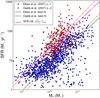Fig. 1

Star formation rate (SFR, in M_⊙ yr^-1) as function of total stellar mass (M_⋆, in M_⊙) in two galaxy samples. The data points are estimates of the star formation rate and stellar mass for samples of galaxies at z ~ 1 (blue circles; Elbaz et al. 2007) and z ~ 2 (red circles; Daddi et al. 2007). The green and purple solid lines indicate the best fits to the data sets at z ~ 1 and z ~ 2 from the original papers. The two red lines indicate our simple star formation model with the best scaling parameters adopted (see text for details).

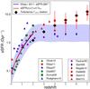Fig. 2

Specific star formation rate (sSFR, in Gyr^-1) as a function of redshift. The various points represent measurements from the literature at M_⋆ ~ 10¹⁰M_⊙; see the references in the legend at the bottom right. We note that we have specifically shown the determinations from (Stark et al. 2013) with their uncertainties (red squares) because there is some controversy as to whether or not there is any evolution in the sSFR with increasing redshift beyond z = 2. Since the slope of the sSFR − M_⋆ relation is approximately zero, the rate at which the sSFR evolves is largely independent of M_⋆, except at the highest masses. The lines represent the best-fit relation from Elbaz et al. (2011) over the redshift range 0 to 2 (blue line) and a simple scenario, sSFR (z) = (1 + z)³/t_H0 (where t_H0 is the Hubble time at z = 0, red line), and the blue squares are the estimates for our hypothesis relating the turbulence to the star formation intensity (see text for details). The blue shaded region represents the scatter in the observed sSFR values (±0.3 dex). This rendition of the evolution of the sSFR is inspired by a similar plot in Weinmann et al. (2011).

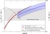Fig. 3

Star formation intensity (Σ_SFR, in M_⊙ yr^-1 kpc^-2) as a function of redshift. The evolution of the generalized Schmidt law (black line) compared to the evolution of abudance-matched star-forming galaxies (i.e., galaxies with co-moving number densities like that of MW mass galaxies in the local Universe) for several types of size evolution (r_e = 3.6(M_⋆/ 5.0 × 10¹⁰)^0.27 – solid red line; r_e = 3.6(1. + z)^-0.55 – upper red dashed line; r_e = 3.6 kpc – lower dashed red line; see van Dokkum et al. 2013, for details). We also show the evolution of the star formation intensity for high redshift galaxies with an sSFR = 2 Gyr^-1, a stellar mass of 5 × 10⁹M_⊙, and a size evolution, r_e = 2.5((1 + z)/3)^-1.2 kpc (blue line and shaded region representing a scatter of ±0.3 dex; see Oesch et al. 2010; Mosleh et al. 2012). The evolution of the stellar mass surface density, Σ_⋆ (M_⊙ kpc^-2; right hand ordinate) of MW-like galaxies (black dashed line) is a factor of about 3 but includes the growth of the bulge as well as the disk (van Dokkum et al. 2013). We also indicate (dotted line) the star formation intensity threshold for local starburst galaxies to drive winds and indicated the possible range of thresholds from local and distant galaxies (Lehnert & Heckman 1996; Heckman 2003; Le Tiran et al. 2011b; Newman et al. 2012a).

The gas supply from accretion is declining and being incorporated into the galaxy with high angular momentum, implying it likely ends up mostly in the outer disk regions (Stewart et al. 2011). This is consistent with the observation that the H i mass surface density does not depend strongly on radius in individual galaxies (Bigiel & Blitz 2012). Thus increasing the angular momentum of the gas as the redshift decreases is a robust way of growing galaxies in a “centrifugally supported” way as suggested in the models of, e.g., Mo et al. (1998). We note however that the relation which best matches the evolution of the sSFR out to ~2 is neither arbitrary nor actually a fit to the data. We would expect the stellar mass surface densities to scale as the Hubble time, t_H0 (Mo et al. 1998) and in fact, that is what sets the zero point for the relation shown in Fig. 2, namely, sSFR(z) = (1 + z)³/t_H0, a relation indistinguishable from that of Elbaz et al. (2011). This scaling comes from cosmological considerations, namely, the change of the structure of dark matter halos (increasing virial radii, masses, etc.) and the overall growth of galaxies. Thus to explain the observed relation requires no free parameters. Moreover, within the context of gas accretion and mass return, one could argue that the scaling we adopted for the generalized Schmidt law analysis is also constrained within the context of our simple hypothesis, although based on parameters estimated for the ISM of galaxies and through comparison with measurements of the sSFR, gas mass surface densities and gas fractions.

We can extend this analysis further. Equation (1) is also a simple relation between the star formation intensity and the stellar and gas mass surface densities, which was obtained by multiplying both sides of the equation by the disk surface area to yield a relation between the SFR and M_⋆ (see Appendix A). Since sSFR(z) evolves as (1 + z)³, this implies that Σ_SFR would also evolve as (1 + z)³ in the context of our model. An evolution of the star formation intensity as (1 + z)³ is shown in Fig. 3, whose zero-point was chosen based on the relation between the disk scale length of local disk galaxies (Fathi et al. 2010) and star formation rates of galaxies with stellar masses similar to the MW (Elbaz et al. 2007; Lara-López et al. 2013). We compare this to the evolution a function of redshift of the star formation intensity of MW-like galaxies selected through abundance matching by van Dokkum et al. (2013), who characterized the size evolution of these MW-like galaxies as a function of redshift and of stellar mass, as shown in Fig. 3 together with, for completeness, a constant size evolution with r_e = 3.6 kpc (the final average size of their sample). The results of our model are in approximate agreement with these observations. Also in Fig. 3 we show the stellar mass surface density evolution of MW-like galaxies (van Dokkum et al. 2013). It only evolves by about a factor of 3 but includes the growth of the bulge so the evolution in the effective mass surface density of the disk would be lower. A small increase in the total stellar mass surface density is important within the context of our model because there is also a dependence on Σ_⋆ and finding little or no evolution in the stellar mass surface density (Barden et al. 2005) suggests that the evolution in Σ_SFR, and hence the sSFR, is mostly due to the changing gas surface densities and gas fractions.

To begin to understand why there is a change in the evolution of the sSFR above and below z ~ 2, we show the evolution of the star formation intensity for galaxies above z ~ 2 assuming the size evolution for a galaxy with M_⋆ ~ 5 × 10⁹M_⊙ and sSFR = 2 Gyr^-1 (approximately the mean sSFR of z ≳ 2 galaxies). The generalized Schmidt law appears to over predict the star formation intensities, suggesting some other regulatory mechanism comes into play. Moreover, the star formation intensities are above the threshold determined for starburst galaxies in the local universe to drive winds (Lehnert & Heckman 1996; Heckman 2003) but this threshold may be somewhat higher for high redshift galaxies (1 M_⊙ yr^-1 kpc^-2; Le Tiran et al. 2011b; Newman et al. 2012a). This suggests that the regulatory mechanism is related to the intensity of star formation (we discuss this subsequently in Sect. 3.3).

We note that such an hypothesis does not preclude observing strong outflows from galaxies at z ≲ 1 − 2 (as they are observed, e.g. Lehnert & Heckman 1996; Rubin et al. 2010, 2014; Coil et al. 2011; Martin et al. 2012; Bouché et al. 2012). Quite the contrary. It just implies that the regions of high star formation intensity are compact and occur only in the circum-nuclear regions and that most galaxies do not drive winds or do so only briefly (e.g. Lehnert & Heckman 1996).

3.2.1. The importance of mass return

We should be cognizant that even though the gas supply from accretion is likely declining, the mass return from the stellar populations within galaxies can be significant and will be especially important for (rotationally supported) galaxies with older stellar populations (~20% or more of their total stellar mass, Leitner & Kravtsov 2011; Snaith et al. 2014). This gas will have an angular momentum content similar to the pre-existing disk, help to maintain the high angular momentum of the accreted gas and aid in growing the disk (Martig & Bournaud 2010). Of course, objections are often raised about the relative contribution of mass return compared to gas accretion, for example, the G-dwarf problem and the abundance of deuterium in the local ISM. However, these problems may not require gas accretion or at least not at significant rates (see e.g. Haywood 2001; Prodanović et al. 2010; Chiappini et al. 2002; Romano et al. 2006; Lagarde et al. 2012; Leitner & Kravtsov 2011; Snaith et al. 2014, for a detailed discussion of these points).

At z = 0, the specific cosmological gas accretion rate is likely significantly below the sSFR for actively star forming galaxies (e.g. Weinmann et al. 2011; Leitner 2012). If such galaxies were forming stars at an approximately constant rate, as observed for the Milky Way over the last 3 Gyr and perhaps much longer (Hernandez et al. 2000; Snaith et al. 2014) and as perhaps implied by the constant gas depletion timescale for local star forming galaxies (Leroy et al. 2013), then the fraction of gas that has been returned is about 20−40% depending on the initial mass function of the age weighted stellar masses (Leitner & Kravtsov 2011). The fraction of the returned gas that is in the molecular phase is likely less than 50% and the distribution of the gas is related to the extent of the stellar disk (Bigiel & Blitz 2012). This emphasizes both the importance of the angular momentum and mass return from the stellar population in determining the gas mass surface densities, which in turn, from our analysis of the generalized Schmidt law, controls the evolution of the specific star formation rate.

3.2.2. Why the break in the sSFR evolution at z ~ 2?

While overall it is likely that the decreasing gas supply plays a fundamental role in determining the z ~ 2 transition redshift, since this redshift, above which the growth of the ensemble of galaxies appears to be self-regulated, and below which angular momentum begins to dictate the decline in the specific stellar mass growth rate with redshift, occurs at approximately the same moment as when the cosmological specific gas accretion rate becomes less than the average sSFR.

However, this is not to imply that gas accretion is necessarily the main driver of the evolution of the sSFR at z ≲ 2 but only determines approximately when the transition occurs. In such a picture, galaxies at z ≲ 2 are living off of their gas-rich earlier phases of evolution (and significant mass return) where star formation is kept inefficient through strong feedback from intense star formation. The high angular momentum of the gas that is being subsequently accreted allows galaxies to preferentially grow their outer disks (Stewart et al. 2011), but this is likely moderated by the low stellar mass surface densities of outer disks because as argued through the generalized Schmidt law, their star formation should be kept relatively inefficient (Blitz & Rosolowsky 2006). Such a picture naturally explains the lack of a significant increase in the central surface densities of star forming galaxies from z ~ 1 (Barden et al. 2005; van Dokkum et al. 2013).

It is not clear if the scenario we are advocating is consistent with “inside-out” evolution and the observation that the H i mass surface density does not depend strongly on radius in individual galaxies (Bigiel & Blitz 2012). However, we may not expect the outer disk to grow more rapidly than the inner disk even if the gas dominates the mass surface density (Bigiel et al. 2010; Bigiel & Blitz 2012) since interstellar pressure plays a significant role in converting gas from the warm neutral phase to the cold molecular phase (Wolfire et al. 1995) and this conversion is related to the stellar mass density (e.g. Blitz & Rosolowsky 2006; Schruba et al. 2011) and of course consistent with the generalized Schmidt law where the stellar mass surface densities play an important role in regulating star formation (Sect. 2 and also, Shi et al. 2011).

The importance of this transition redshift and angular momentum is emphasized by a number of observations of the stellar populations of both the Milky Way and other nearby galaxies. Before the z ~ 2 transition, the Milky Way, formed its thick disk, had high star formation intensities and high stellar velocity dispersions, and its disk had a short scale length (e.g. Haywood et al. 2013,and references therein). The low scatter in [α/Fe] as a function of age and the rapid decrease in [α/Fe] with time of the thick disk suggests that the mixing of metals was very efficient and the increase in metallicity was dominated by core collapse supernovae. In addition, as the thick disk evolved, its stellar velocity dispersion decreased (Haywood et al. 2013). The young Milky Way formed during an intense burst of star formation with increasing angular momentum which gradually died down over about 4 Gyr and undoubtedly experience strong feedback and high turbulence (Haywood et al. 2013; Snaith et al. 2014; Lehnert et al. 2014). At around the transition redshift, ≈10 Gyr ago, the abundance ratios and ages of stars suggest that the MW starts to form stars in an outer thin disk while the inner disk was still thick and as did perhaps the outer disks of other nearby spiral galaxies (Ferguson & Johnson 2001; Vlajić et al. 2009; Barker et al. 2011; Haywood et al. 2013). Overall, the results on the Milky Way suggest an early phase of low angular momentum gas accretion which fueled intense star formation with a short scale length but large scale height followed by a phase of quiescent growth with a longer scale length and a small scale height. These are core arguments in our scenario and appear to be mimicked in the star formation history of the MW and other nearby galaxies. Such a picture is in agreement with our analysis shown in Fig. 3. At z ≳ 2, the star formation intensity of galaxies is sufficiently high to drive strong winds and create a highly turbulent ISM as observed (Newman et al. 2012a; Lehnert et al. 2013).

Care must be taken in arguing for a continuous scenario of galaxy evolution over the last ~13 Gyr. It is extremely likely that the evolution of the sSFR of the ensemble of galaxies is driven by changing populations at different redshifts. While the Milky Way shows evidence for continued growth over the age of the universe (Haywood et al. 2013; van Dokkum et al. 2013), massive galaxies, in particular, have stellar age distributions dominated by old populations which formed relatively quickly (e.g. Johansson et al. 2012) and have high stellar surface densities (e.g. Shen et al. 2003; Bernardi et al. 2010; Carollo et al. 2013) consistent with them growing primarily through high intensity star formation with strong feedback.

In addition, using the evolution of the sSFR itself to constrain the growth of mass in the ensemble of galaxies also suggests that there is a possible dichotomy in the growth rates of galaxies as a function of mass, in that more massive galaxies grew rapidly above z ~ 2 (Leitner 2012). The high intensity star formation we observe is consistent with this dichotomy but within the context of our strong feedback scenario would also predict that the duty cycle of star formation is relatively small (~10−20%) at high redshifts (Verma et al. 2007; Davies et al. 2012). Strong feedback limiting the duration of the duty cycle may be consistent with a flat or slowly increasing sSFR with redshift (Wyithe et al. 2014) as are the general arguments we have made here. Given that our analysis indicates that feedback processes might regulate the SFR in galaxies at high redshift, we now discuss two possible mechanisms for doing so.

3.3. Mechanical and radiative self-regulated star formation

It is possible that star formation is limited by its own mechanical and radiative energy output (self-regulation). On global scales, there are (at least) two possible mechanisms whereby the energy injected by massive stars could limit the sSFR. One balances the pressure (thrust) generated by the thermalized hot plasma due to the combined action of stellar winds and supernovae plus radiation pressure with the overall galactic mid-plane hydrostatic pressure. In the other, the high turbulence in the dense molecular medium is sustained by a mass and energy exchange within the ISM driven by the energy output of the young stars, which maintains distant galaxies near or on the line of instability (i.e. Toomre Q ~ 1). It is this mass and energy exchange that ultimately regulates the sSFR of distant galaxies. We will discuss these two in turn.

3.3.1. Wind and radiative thrust balancing hydrostatic pressure

We hypothesize that the mechanical energy from massive stars is controlling the overall pressure, and in such a situation, we would expect the pressure to increase linearly with the star-formation intensity. The ultimate limit in the pressure driven by the mass and energy output of massive stars is reached when it balances or exceeds the mid-plane pressure – similar to what has been hypothesized to limit the star-formation intensity in nearby starburst galaxies (Lehnert & Heckman 1996).

The pressure due to the mechanical energy of intense star formation is P_feedback ∝ Ṁ^1/2Ė^1/2 $R_{⋆}^{-2}$ $\hbox{$R_{\star}^{-2}$}$ , where P_feedback is the gas thermal pressure generated by the effects of massive stars, Ṁ is the mass loss, Ė is the mechanical energy output and R_⋆ is the radius over which the energy and mass output occurs (e.g. Strickland & Heckman 2009). The constant of proportionality depends on the opening angle (or geometry) of the flow, the thermalization efficiency of the mechanical energy output, the mass entrainment rate in the wind, and how well this energy and mass couples to the surrounding ISM. Constraining these dependencies is difficult. From observations of nearby starburst galaxies, the opening angle is approximately, π (Heckman et al. 1990; Lehnert & Heckman 1996). The thermalization efficiency is likely to be high, about 0.3−1.0 (Strickland & Heckman 2009) and the mass loading (ratio of total outflow mass and total stellar mass ejected through stellar winds and supernovae) high as well, about 4−20 (e.g., Moran et al. 1999; Bouché et al. 2012). In high redshift galaxies, the mass loading may be higher than generally observed in nearby starbursts owing to higher gas column densities and larger disk thicknesses (Lagos et al. 2013).

We can estimate the mechanical energy and mass output rate from star formation using stellar population synthesis models (Leitherer et al. 1999). Adopting an equilibrium mass and energy output rate for continuous star formation over 10⁸ yrs, we estimate pressures of 3.6 × 10^-10 dyne cm^-2 for 1 M_⊙ yr^-1 kpc^-2. Another estimate can be made from previous studies which found that the outflow rate is roughly equal to the SFR. This implies a mass loading/entrainment factor about 4 or a pressure of 7.2 × 10^-10 dyne cm^-2 (Moran et al. 1999; Strickland & Heckman 2009) but as noted previously, it could be higher as it scales with the square root of the mass loading factor.

The hydrostatic pressure depends on the gas and stellar mass surface densities (which are related through the gas fraction) and adopting the more general relation, on the ratio of the gas to stellar velocity dispersions (Sect. 2.2.3; Elmegreen 1993). We therefore need to estimate mass surface densities, gas fractions, star formation rates and galaxy sizes.

Measurements of stellar mass surface densities in star-forming galaxies at z ≈ 1−6 estimate ~100−2000 M_⊙ pc^-2 (e.g. Barden et al. 2005; Yuma et al. 2011; Förster Schreiber et al. 2011; Mosleh et al. 2012) and high gas fractions (e.g. Tacconi et al. 2013). At z ~ 5−7, galaxies are estimated to have a very high sSFR, ≈10 Gyr^-1 (Stark et al. 2013), although the uncertainties in this value are large. The observed fiducial stellar mass of these galaxies is ~10⁹M_⊙ and their half-light radius ~0.5 kpc (Mosleh et al. 2012). These are intensely star forming galaxies, with Σ_SFR ≈ 6 M_⊙ yr^-1 kpc^-2 and high stellar mass surface densities, Σ_⋆ ≈ 600 M_⊙ pc^-2. The more massive galaxies with the smallest half-light radii at these redshifts can reach Σ_⋆ ≈ 1000−2000 M_⊙ pc^-2, similar to early type galaxies at moderate to low redshifts (Carollo et al. 2013).

At lower redshifts, z ≈ 2, the average mass surface density is much lower, thus making it easier in this scenario for the mechanical energy to regulate the star formation through pressure. In galaxies at z ≈ 2−3, Σ_⋆ ≈ 200−300 M_⊙ pc^-2 (Förster Schreiber et al. 2011; Mosleh et al. 2012) and their average Σ_SFR ≈ 1 M_⊙ yr^-1 kpc^-2 (Lehnert et al. 2013). The gas fractions of galaxies at z ~ 5−7 are unknown, but at z ~ 2, they are observed to be f_g = 30−70% (Tacconi et al. 2010, 2013). As already discussed (Sect. 2), we do not know the velocity dispersions of the gas relative to the stars and their ratios could easily range from 0.2 to 1.

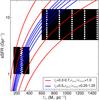Fig. 4

Specific star formation rate (sSFR, in Gyr^-1) as a function of the stellar mass surface density (Σ_⋆, in M_⊙ pc^-2) as predicted by a simple relation where the hydrostatic pressure and the thrust of the mechanical energy generated by intense star formation are equal. To span a range of possible sSFR in such a scenario, we vary the input values of the gas fraction, f_g, or the velocity dispersion ratio of the gas and the stars, σ_gas/σ_stars. The red solid lines represent this equality for a range of gas fractions, f_g = 0.3 to 0.7, and for a constant σ_gas/σ_stars = 1, while the blue lines represent this equality for a constant gas fraction, f_g = 0.3, and a range of σ_gas/σ_stars = 0.25−1.25 in steps of 0.25. The hatched regions indicate approximately the observed range of stellar mass surface densities and sSFR at z ~ 2 (diagonally hatched region) and z ~ 5−7 (cross-hatched region; see text for details).

When we simply equate the hydrostatic pressure (Sect. 2.2.3) and the “feedback pressure”, we find reasonable agreement with observed stellar mass surface densities and sSFR for galaxies at z ~ 2 and z ~ 5−7 (Fig. 4), for a reasonable range of f_g and σ_gas/σ_stars, assuming a thermalization efficiency of 0.5, a mass loading factor of 10 or an outflow rate of 2−3 times the SFR.

We emphasize that within the context of this simple calculation, the mass loading factor and thermalization efficiency are degenerate and that it is the product of the square root of their values that results in the estimate of the mechanical energy. Since the half-light radius of galaxies at constant stellar mass evolves systematically with redshift, such a model provides a reasonable explanation for the sSFR at z ≈ 2−7. This simple scenario predicts a strong decline in the sSFR with stellar mass surface density and some of the curves in Fig. 4 for high gas fractions and large ratios of gas to stellar velocity dispersions lie above the region occupied by distant galaxies.

The equivalent of requiring the feedback pressure to balance or exceed the hydrostatic pressure is to say the gas is only marginally bound. Obviously, this is an extreme assumption and unlikely to hold true over the entire ISM simultaneously. Therefore, it is perhaps more appropriate to consider this as a viable mechanism for limiting the values that the SFR can sustain.

Using the mechanical energy output from young stars to limit the sSFR is purely empirical in that it does not make predictions of the evolution of the sSFR but only provides upper limits or ranges for it, which depend on parameters that can solely be determined observationally. In some sense, it is similar to phenomenological models of galaxy evolution, though with significantly less complication, in that it attempts physical descriptions of processes that are otherwise difficult to constrain, such as the star formation efficiency or the relation between star formation intensity and gas surface density (e.g. Behroozi et al. 2013; Feldmann 2013). While we have not tried to constrain our input parameters by fitting the evolution of the sSFR, and rather adopted values consistent with observations, it indicates that this type of scenario works reasonably well in describing the evolution of the sSFR.

Since the mechanical energy input depends on the mass loading and the thermalization efficiency, it is quite likely that as the galaxies grow less compact, the area covered by the intense star formation decreases and the overall pressure of the ISM will drop in lock step with declining hydrostatic pressure. However, galaxies at z = 2−4 exhibit clumpy star formation with ample evidence for driving significant outflows (Le Tiran et al. 2011b; Newman et al. 2012a,b) and the thermal pressure of the warm ionized medium in these clumpy galaxies appears high (similar to nearby starburst galaxies driving winds; Lehnert et al. 2009, 2013; Le Tiran et al. 2011a) and perhaps also have high turbulent pressures in the cold molecular medium (Renaud et al. 2012; Lehnert et al. 2013). This clumpy structure likely leads efficient thermalization and coupling of the mechanical energy output of young stars to the surrounding ISM, allowing the mechanical (and radiative) energy to influence the gravitational collapse of dense gas and therefore the SFR and the sSFR. These individual clumps of intense star formation are akin to individual galaxies at z ≈ 6, in the sense that they are similarly compact and that the most massive ones can have similar stellar masses (Elmegreen et al. 2009b,a; Förster Schreiber et al. 2011) and sSFR (Guo et al. 2012), and they show evidence for strong stellar feedback (e.g. Le Tiran et al. 2011b; Newman et al. 2012a). These similarities and relationships may allow for similar regulation of star formation and baryonic growth but less efficiently in the case where the most intense star formation covers the entire disk, because of the lower covering factor of similarly intense star formation within the (significantly larger) disk (Förster Schreiber et al. 2011; Guo et al. 2012).

Certainly, with reasonable parameters, finding a decrease of about a factor of 3 in the sSFR with stellar mass surface density is consistent with the overall trend observed (Fig. 4). The normalization appears high compared to the data, but it is important to note that our underlying assumption of an almost unbound disk is quite extreme. We would expect such a model to explain the most intensely star forming galaxies, perhaps not the typical ones.

3.3.2. Turbulent pressure and the line of stability (Q ~ 1)

Galaxies at high redshift, z ≳ 1, have broad optical emission lines (velocity dispersions ~30−200 km s^-1; e.g., Epinat et al. 2009, 2010; Förster Schreiber et al. 2009; Law et al. 2009; Kassin et al. 2012) which may be related to their high observed star-formation intensities (Lehnert et al. 2009, 2013). In Lehnert et al. (2013), we proposed that there is a mass and energy exchange in the ISM of distant galaxies between the warm ionized medium and the cold molecular medium. The high pressures observed in the warm ionized medium (and its likely similarity with the hot X-ray emitting gas) implies that much of the ionized gas will quickly become cold neutral gas and, if it contains dust, cold molecular gas (Wolfire et al. 1995; Feldmann et al. 2012). This rapid phase change under high pressures allows the cold molecular gas to “capture” the kinematics of the warm ionized gas. In such a scenario, the molecular gas acquires much of the turbulent motions observed in the optical emission line gas and since the molecular phase dominates the overall mass surface density, it may have sufficient turbulent pressure to approximately balance gravity over large scales. This balance then leads to a situation where galaxies are driven towards the line of stability for global star formation (i.e., a Toomre instability criterion of Q ~ 1).

In such a picture, if the star formation intensity were to increase, the galaxy would move beyond the line of stability and star formation would be suppressed; if the star formation intensity falls, the galaxy would become globally more unstable and thereby increase its star formation intensity. This naturally leads to the regulation of star formation to a narrow range around the line of instability, Q ~ 1.

A sufficiently high gas content is needed to regulate star formation. Star formation, as observed in local galaxies, becomes regulated by the local balance of turbulent energy dissipation, energy released by gravitational collapse and instability, and energy injected by the stellar population. Such balance would no longer be maintained when the gas content decreases to the point when it is either insufficient to fuel the necessary high star formation intensities, when the outflow of gas and energy are significant enough to make the energy input from massive stars unable to sustain high levels of disk turbulence, or when the turbulent dissipation timescale becomes long enough such that star formation becomes inefficient (efficient dissipation is necessary to sustain intense star formation). The disk would then settle over time as the gas mass surface densities decrease (perhaps as observed, e.g. Epinat et al. 2010; Kassin et al. 2012).

If we assume that galaxies lie near the line of instability and that the turbulence in the ISM is driven by intense star formation of the form, σ_gas = ϵΣ^1/2 (where ϵ is the coupling factor between the star formation intensity, in units of 1 M_⊙ yr^-1 kpc^-2, and σ_gas is the velocity dispersion of the gas in km s^-1) then, applying the effective Toomre criterion (Q_total^-1 = Q_stars^-1 + Q_gas^-1; Wang & Silk 1994), we find, $sSFR = (\frac{Σ_{SFR}}{Σ_{⋆}}) = {(\frac{π G Q_{total}}{κϵ})}^{2} Σ_{⋆} (\frac{f_{g}}{1 - f_{g}} + \frac{σ_{gas}}{σ_{⋆}}) 2$ $\begin{equation} \nonumber {\it sSFR} = \left(\frac{\Sigma_{\rm SFR}}{\Sigma_{\star}}\right) = \left(\frac{\pi {\rm G} {\rm Q}_{\rm total}}{\kappa \epsilon}\right)^{2} \Sigma_{\star}\left(\frac{{\rm f}_{\rm g}}{1-{\rm f}_{\rm g}} + \frac{\sigma_{\rm gas}}{\sigma_\star}\right)^{2} \end{equation}$ (2)where κ is the epicyclic frequency (taken to be $\sqrt{2}$ $\hbox{$\sqrt{2}$}$ Ω, with Ω the angular frequency, and assuming a constant circular velocity) and f_g is the gas fraction.

The derivation assumes that the total sSFR = SFR/M_⋆ = Σ_SFR/ Σ_⋆. In Lehnert et al. (2009, 2013), we estimated that an efficiency factor of 140 km s^-1 (M_⊙ yr^-1 kpc^-2)^−1/2 was necessary to explain the relation between the star formation intensity and the velocity dispersion in galaxies at z ≈ 2 (Lehnert et al. 2013). However, this factor could be 30% lower, as we generally did not correct for extinction in the sample, and the star formation intensities could be higher by a factor of about 2 (Lehnert et al. 2009, 2014). In Fig. 2, we assumed 120 km s^-1 (M_⊙ yr^-1 kpc^-2)^−1/2 to take into account that the efficiency is likely lower (Lehnert et al. 2014).

We note that this analysis is closely related to that given in Sect. 2 based on the generalized Schmidt law, which we used to estimate the relationship between the SFR and stellar mass (Fig. 1) since both arguments are ultimately related to the pressure in the ISM.

The resulting relation shows a reasonable agreement with the observed values for both sSFR and stellar mass surface density of distant galaxies (Fig. 5) and for the evolution of the sSFR with redshift (Fig. 2). For the latter, we scaled the sizes of the galaxies by (1 + z)^-1.2 for a constant stellar mass of 10^9.3M_⊙, a gas fraction of 0.5, a ratio of gas to stellar velocity dispersion of 1 and assumed a constant epicyclic frequency consistent with those estimated at z ≈ 2−3 (Lehnert et al. 2013), as we expect it to only vary by a factor of a few with redshift.

Since we have some freedom of choice in the parameters we adopt, the agreement may seem rather fortuitous. On the other hand, both models, one in which supernovae and strong stellar winds determine the pressure and balances hydrostatic equilibrium, and the other, where star formation drives strong turbulence holding galaxies near the line of instability, provide reasonable evolution in the sSFR with stellar mass surface density and redshift (although the thrust balancing the hydrostatic pressure is a very extreme assumption). The results of both models emphasize the important role that self-regulation of star formation plays in balancing the relative rate of growth of galaxies and the high gas fractions that are necessary to allow this stellar feedback to couple efficiently to the ISM (Lehnert et al. 2013).

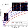Fig. 5

Specific star formation rate (sSFR, in Gyr^-1) as a function of stellar mass surface density (Σ_⋆, in M_⊙ pc^-2), for the hypothesis that the star formation drives galaxies towards the line of stability against star formation (Toomre parameter, Q = 1) as described in the text. The red and blue solid lines represents the sSFR where the energy input from massive stars generates enough turbulence to drive the global ISM towards Q ~ 1. The red solid lines represent where Q ~ 1 for a range of gas fractions (f_g = 0.3 to 0.7) and for a constant σ_gas/σ_stars = 1, while the blue lines represent where Q = 1 for a constant gas fraction (f_g = 0.5) and σ_gas/σ_stars = 1, but now for a range of energy input from massive stars into the turbulence of the ISM, ϵ = 100–160 km s^-1 kpc yr $^{1 / 2} M_{⊙}^{- 1 / 2}$ $\hbox{$^{1/2}~M_{\sun}^{-1/2}$}$ , where ϵ is the coupling between the star formation intensity and the velocity dispersion (Lehnert et al. 2009, 2013). The predicted sSFR values increase with increasing gas fraction but decrease with increasing ϵ. The hatched regions are the same as in Fig. 4.

3.3.3. Comparison with other sSFR evolution models

Although there have been other studies of the possible underlying processes which may dictate the sSFR − M_⋆ relation and its evolution over cosmic time, there is as yet no consensus on what these may be. Only a few studies have suggested that self regulation through interstellar gas pressure is the primary driver of the observed evolution (e.g. Birnboim & Balberg 2013). The study of Dutton et al. (2010) finds that the evolution of the sSFR is driven by the details of the gas accretion history, and by increasing both the gas surface densities of molecular gas and the ratio of the molecular to atomic gas mass (Blitz & Rosolowsky 2006). Surprisingly, they do not predict an evolution of the gas fraction, except at the highest redshifts. Other models suggest that the evolution at z ≲ 2−4 can be entirely explained by changes in the specific gas accretion rate (e.g. Dutton et al. 2010; Kang et al. 2010). Interestingly, it is over this redshift range that there is almost no evolution in the mean density of halos at constant halo mass within 20 kpc radius despite the large growth in the virial radius (Weinmann et al. 2013). At z ≳ 4, Khochfar & Silk (2011) suggest that the sSFR is driven by the star-formation efficiency being dependent on the mode of accretion – mergers or cosmological gas accretion. Their model predicts a preponderance of mergers at high redshift. Weinmann et al. (2011), in a comprehensive study, found a number of ways in which a plateau, or a slowly rising sSFR at z ≳ 2 may be explicable. The effects they suggested include a reduced star-formation efficiency/enhanced feedback, prohibiting the gas from forming stars, efficiently ejecting the gas which is subsequently accreted by more massive halos, or through an enhanced growth rate of massive galaxies.

The advantage of our simple scenario, in comparison, is that the gas accretion history has little impact on the evolution of the sSFR with cosmic time, only that sufficient gas needs to be accreted at high redshifts to allow the gas content to build up high mass surface density galaxies at high redshift, that the angular momentum of the accreted gas generally increases with decreasing redshift, and that the rate of gas accretion then declines with decreasing redshift. The evolution of the sSFR in our model is determined by the change in the angular momentum content of the accreted gas (Dubois et al. 2013; Danovich et al. 2015) and how the gas and stellar mass surface densities are limited by the energy and mass output of massive stars. With these two processes, the range of gas/stellar mass surface densities observed in galaxies as a function of redshift may be explained. The star formation intensities are related to the gas mass surface density through the well-known simple relation between the two with an exponent of the order of unity (Leroy et al. 2013). Higher gas mass surface densities lead to higher star-formation intensities, which in turn lead to higher stellar mass surface densities, both of which are limited by feedback from massive stars but whose overall evolution is driven by the angular momentum with which gas is accreted. This is naturally proportional to both the gas fraction, total gas content and total mass of galaxies. It requires little further fine tuning in that at high redshift (z ≳ 2) the gas supply is in excess of that needed to support star formation and that at low redshift (z ≲ 2) centrifugal support is important in limiting the ultimate surface density (or volume density) of gas in galaxies. Importantly, it is this natural limiting of the surface densities through the pressure that gives the SFR − M_⋆ relation its slope of one – consistent within the uncertainties with studies of the SFR − M_⋆ relation.

4. Summary

We find that the SFR − M_⋆ relationship and the evolution of specific star formation rates with cosmic time are consistent with a scenario where the relative growth rates of galaxies are set by the interplay of the stellar and gas mass surface densities and by self-regulated star formation. The stellar mass surface densities are related to the gas mass surface densities through the relationship between star-formation intensity and gas mass surface density, whose exponent is approximately unity (Leroy et al. 2013). It is the angular momentum of the accreted gas that will help set the ultimate limit on the intensity of the star formation by influencing the surface densities the gas is able to reach. Feedback and self-regulation from young stars help keep the star formation inefficient. The slope of the SFR − M_⋆ relationship, which is a ridge line in the SFR − M_⋆ plane, can successfully be reproduced in a scenario where the global SFR in galaxies is related to the overall pressure in the ISM which is itself due to the intense star formation (Hopkins et al. 2013). This also implies that, even when the gas supply through cosmic accretion is very large, the sSFR cannot increase without bound, but only slowly, with limits set by feedback from intense star formation within the context of the high stellar mass surface densities observed in the early universe (z ≳ 2 − 3).

The decrease in sSFR at z ≲ 2 implies that the gas mass surface density and gas supply are reduced below the levels necessary to maintain the high intensity, compact star formation as observed. The growth of the ensemble of galaxies is no longer self-regulated by star formation. Now, with the gas supply below this threshold, processes internal to the galaxy or the mode of accretion become important. In a simple cosmological model, the radius of a centrifugally supported gaseous disk is expected to evolve as (1 + z)^-1.5 and thus the mass surface density (at constant mass) as (1 + z)³/t_H0 – similar to the observed rate of decline of the sSFR with redshift at z ≲ 2 (Oliver et al. 2010; Elbaz et al. 2011). Thus we hypothesize that what limits the star formation efficiency and baryon content of galaxies to the level necessary to explain the observed evolution of the sSFR with cosmic time is a combination of the gas accretion rate (whether it is generally higher or lower than the sSFR which then established the transition redshift between the two regimes controlling the sSFR), the angular momentum of the accreted gas (which then determines both how compact the galaxy is at a constant stellar mass and the evolution of its gas fraction), and self-regulating star formation and feedback through regulating the pressure of the ISM. Obviously, more work is needed beyond these simple ideas to gauge if the scenario we have advocated is consistent with other constraints on galaxy evolution (e.g. cosmic star-formation history, size evolution of galaxies, etc.).

Acknowledgments

M.D.L. wishes to thank Yohan Dubois, Gary Mamon, Sébastian Peirani, and Marta Volonteri for interesting discussions, and Christophe Pichon and Mike Fall for the engaging talks at the IAP 75th anniversary conference which helped some of these ideas to congeal. We especially thank David Elbaz, Gary Mamon, and Joe Silk for their critical reading of and helpful comments on this manuscript. We thank our former co-author N. P. H. Nesvadba for her participation in the preparation of this manuscript.

References

Abramson, L. E., Kelson, D. D., Dressler, A., et al. 2014, ApJ, 785, L36 [NASA ADS] [CrossRef] [Google Scholar]
Agertz, O., Lake, G., Teyssier, R., et al. 2009, MNRAS, 392, 294 [NASA ADS] [CrossRef] [Google Scholar]
Aravena, M., Carilli, C., Daddi, E., et al. 2010, ApJ, 718, 177 [NASA ADS] [CrossRef] [Google Scholar]
Baldry, I. K., Glazebrook, K., & Driver, S. P. 2008, MNRAS, 388, 945 [NASA ADS] [Google Scholar]
Barden, M., Rix, H.-W., Somerville, R. S., et al. 2005, ApJ, 635, 959 [NASA ADS] [CrossRef] [Google Scholar]
Barker, M. K., Ferguson, A. M. N., Cole, A. A., et al. 2011, MNRAS, 410, 504 [NASA ADS] [CrossRef] [Google Scholar]
Behroozi, P. S., Wechsler, R. H., & Conroy, C. 2013, ApJ, 770, 57 [NASA ADS] [CrossRef] [Google Scholar]
Bernardi, M., Shankar, F., Hyde, J. B., et al. 2010, MNRAS, 404, 2087 [NASA ADS] [Google Scholar]
Bigiel, F., & Blitz, L. 2012, ApJ, 756, 183 [NASA ADS] [CrossRef] [Google Scholar]
Bigiel, F., Leroy, A., Walter, F., et al. 2010, AJ, 140, 1194 [NASA ADS] [CrossRef] [Google Scholar]
Bird, J. C., Kazantzidis, S., Weinberg, D. H., et al. 2013, ApJ, 773, 43 [NASA ADS] [CrossRef] [MathSciNet] [Google Scholar]
Birnboim, Y., & Balberg, S. 2013, ArXiv e-prints [arXiv:1311.1206] [Google Scholar]
Blitz, L., & Rosolowsky, E. 2006, ApJ, 650, 933 [NASA ADS] [CrossRef] [Google Scholar]
Bond, N. A., Ivezić, Ž., Sesar, B., et al. 2010, ApJ, 716, 1 [NASA ADS] [CrossRef] [Google Scholar]
Bottema, R. 1993, A&A, 275, 16 [NASA ADS] [Google Scholar]
Bouché, N., Cresci, G., Davies, R., et al. 2007, ApJ, 671, 303 [NASA ADS] [CrossRef] [Google Scholar]
Bouché, N., Dekel, A., Genzel, R., et al. 2010, ApJ, 718, 1001 [NASA ADS] [CrossRef] [Google Scholar]
Bouché, N., Hohensee, W., Vargas, R., et al. 2012, MNRAS, 426, 801 [NASA ADS] [CrossRef] [Google Scholar]
Bovy, J., Rix, H.-W., Hogg, D. W., et al. 2012, ApJ, 755, 115 [NASA ADS] [CrossRef] [Google Scholar]
Brook, C. B., Stinson, G. S., Gibson, B. K., et al. 2012, MNRAS, 426, 690 [NASA ADS] [CrossRef] [Google Scholar]
Carollo, C. M., Bschorr, T. J., Renzini, A., et al. 2013, ApJ, 773, 112 [NASA ADS] [CrossRef] [Google Scholar]
Ceverino, D., Dekel, A., Mandelker, N., et al. 2012, MNRAS, 420, 3490 [NASA ADS] [CrossRef] [Google Scholar]
Chiappini, C., Renda, A., & Matteucci, F. 2002, A&A, 395, 789 [NASA ADS] [CrossRef] [EDP Sciences] [Google Scholar]
Codis, S., Pichon, C., Devriendt, J., et al. 2012, MNRAS, 427, 3320 [NASA ADS] [CrossRef] [Google Scholar]
Coil, A. L., Weiner, B. J., Holz, D. E., et al. 2011, ApJ, 743, 46 [NASA ADS] [CrossRef] [Google Scholar]
Daddi, E., Dickinson, M., Morrison, G., et al. 2007, ApJ, 670, 156 [NASA ADS] [CrossRef] [Google Scholar]
Daddi, E., Dannerbauer, H., Krips, M., et al. 2009, ApJ, 695, L176 [NASA ADS] [CrossRef] [Google Scholar]
Daddi, E., Bournaud, F., Walter, F., et al. 2010, ApJ, 713, 686 [NASA ADS] [CrossRef] [Google Scholar]
Dannerbauer, H., Daddi, E., Riechers, D. A., et al. 2009, ApJ, 698, L178 [NASA ADS] [CrossRef] [Google Scholar]
Danovich, M., Dekel, A., Hahn, O., Ceverino, D., & Primack, J. 2015, MNRAS, 449, 2087 [NASA ADS] [CrossRef] [Google Scholar]
Davé, R., Oppenheimer, B. D., & Finlator, K. 2011, MNRAS, 415, 11 [NASA ADS] [CrossRef] [Google Scholar]
Davies, L. J. M., Bremer, M. N., Stanway, E. R., et al. 2012, MNRAS, 425, 153 [NASA ADS] [CrossRef] [Google Scholar]
Dekel, A., Sari, R., & Ceverino, D. 2009, ApJ, 703, 785 [Google Scholar]
Dekel, A., Zolotov, A., Tweed, D., et al. 2013, MNRAS, 435, 999 [NASA ADS] [CrossRef] [Google Scholar]
Dopita, M. A., & Ryder, S. D. 1994, ApJ, 430, 163 [NASA ADS] [CrossRef] [Google Scholar]
Dubois, Y., Pichon, C., Devriendt, J., et al. 2013, MNRAS, 428, 2885 [NASA ADS] [CrossRef] [Google Scholar]
Dunne, L., Ivison, R. J., Maddox, S., et al. 2009, MNRAS, 394, 3 [NASA ADS] [CrossRef] [Google Scholar]
Dutton, A. A., van den Bosch, F. C., & Dekel, A. 2010, MNRAS, 405, 1690 [NASA ADS] [Google Scholar]
Elbaz, D., Daddi, E., Le Borgne, D., et al. 2007, A&A, 468, 33 [NASA ADS] [CrossRef] [EDP Sciences] [Google Scholar]
Elbaz, D., Dickinson, M., Hwang, H. S., et al. 2011, A&A, 533, A119 [NASA ADS] [CrossRef] [EDP Sciences] [Google Scholar]
Elmegreen, B. G. 1989, ApJ, 338, 178 [NASA ADS] [CrossRef] [Google Scholar]
Elmegreen, B. G. 1993, ApJ, 411, 170 [NASA ADS] [CrossRef] [Google Scholar]
Elmegreen, D. M., & Elmegreen, B. G. 2006, ApJ, 651, 676 [NASA ADS] [CrossRef] [Google Scholar]
Elmegreen, B. G., Elmegreen, D. M., Fernandez, M. X., & Lemonias, J. J. 2009a, ApJ, 692, 12 [NASA ADS] [CrossRef] [Google Scholar]
Elmegreen, D. M., Elmegreen, B. G., Marcus, M. T., et al. 2009b, ApJ, 701, 306 [NASA ADS] [CrossRef] [Google Scholar]
Epinat, B., Contini, T., Le Fèvre, O., et al. 2009, A&A, 504, 789 [NASA ADS] [CrossRef] [EDP Sciences] [Google Scholar]
Epinat, B., Amram, P., Balkowski, C., & Marcelin, M. 2010, MNRAS, 401, 2113 [NASA ADS] [CrossRef] [Google Scholar]
Fathi, K., Allen, M., Boch, T., Hatziminaoglou, E., & Peletier, R. F. 2010, MNRAS, 406, 1595 [NASA ADS] [Google Scholar]
Feldmann, R. 2013, MNRAS, 433, 1910 [NASA ADS] [CrossRef] [Google Scholar]
Feldmann, R., Hernandez, J., & Gnedin, N. Y. 2012, ApJ, 761, 167 [NASA ADS] [CrossRef] [Google Scholar]
Ferguson, A. M. N., & Johnson, R. A. 2001, ApJ, 559, L13 [NASA ADS] [CrossRef] [Google Scholar]
Feulner, G., Gabasch, A., Salvato, M., et al. 2005, ApJ, 633, L9 [NASA ADS] [CrossRef] [Google Scholar]
Förster Schreiber, N. M., Genzel, R., Bouché, N., et al. 2009, ApJ, 706, 1364 [NASA ADS] [CrossRef] [Google Scholar]
Förster Schreiber, N. M., Shapley, A. E., Erb, D. K., et al. 2011, ApJ, 731, 65 [NASA ADS] [CrossRef] [Google Scholar]
Guo, Y., Giavalisco, M., Ferguson, H. C., Cassata, P., & Koekemoer, A. M. 2012, ApJ, 757, 120 [NASA ADS] [CrossRef] [Google Scholar]
Haywood, M. 2001, MNRAS, 325, 1365 [NASA ADS] [CrossRef] [Google Scholar]
Haywood, M., Di Matteo, P., Lehnert, M. D., Katz, D., & Gómez, A. 2013, A&A, 560, A109 [NASA ADS] [CrossRef] [EDP Sciences] [Google Scholar]
Heckman, T. M. 2003, Rev. Mex. Astron. Astrofis. Conf. Ser., 17, 47 [Google Scholar]
Heckman, T. M., Armus, L., & Miley, G. K. 1990, ApJS, 74, 833 [NASA ADS] [CrossRef] [Google Scholar]
Hernandez, X., Valls-Gabaud, D., & Gilmore, G. 2000, MNRAS, 316, 605 [NASA ADS] [CrossRef] [Google Scholar]
Hopkins, P. F., Kereš, D., & Murray, N. 2013, MNRAS, 432, 2639 [NASA ADS] [CrossRef] [Google Scholar]
Inoue, T., & Fukui, Y. 2013, ApJ, 774, L31 [NASA ADS] [CrossRef] [Google Scholar]
Johansson, J., Thomas, D., & Maraston, C. 2012, MNRAS, 421, 1908 [NASA ADS] [CrossRef] [Google Scholar]
Jurić, M., Ivezić, Ž., Brooks, A., et al. 2008, ApJ, 673, 864 [NASA ADS] [CrossRef] [MathSciNet] [Google Scholar]
Kang, X., Lin, W. P., Skibba, R., & Chen, D. N. 2010, ApJ, 713, 1301 [NASA ADS] [CrossRef] [Google Scholar]
Karim, A., Schinnerer, E., Martínez-Sansigre, A., et al. 2011, ApJ, 730, 61 [NASA ADS] [CrossRef] [Google Scholar]
Kassin, S. A., Weiner, B. J., Faber, S. M., et al. 2012, ApJ, 758, 106 [NASA ADS] [CrossRef] [Google Scholar]
Khochfar, S., & Silk, J. 2011, MNRAS, 410, L42 [NASA ADS] [Google Scholar]
Lagarde, N., Romano, D., Charbonnel, C., et al. 2012, A&A, 542, A62 [NASA ADS] [CrossRef] [EDP Sciences] [Google Scholar]
Lagos, C. D. P., Lacey, C. G., & Baugh, C. M. 2013, MNRAS, 436, 1787 [NASA ADS] [CrossRef] [Google Scholar]
Lara-López, M. A., Hopkins, A. M., López-Sánchez, A. R., et al. 2013, MNRAS, 434, 451 [NASA ADS] [CrossRef] [Google Scholar]
Law, D. R., Steidel, C. C., Erb, D. K., et al. 2009, ApJ, 697, 2057 [NASA ADS] [CrossRef] [Google Scholar]
Le Tiran, L., Lehnert, M. D., Di Matteo, P., Nesvadba, N. P. H., & van Driel, W. 2011a, A&A, 530, L6 [NASA ADS] [CrossRef] [EDP Sciences] [Google Scholar]
Le Tiran, L., Lehnert, M. D., van Driel, W., Nesvadba, N. P. H., & Di Matteo, P. 2011b, A&A, 534, L4 [NASA ADS] [CrossRef] [EDP Sciences] [Google Scholar]
Lehnert, M. D., & Heckman, T. M. 1996, ApJ, 462, 651 [NASA ADS] [CrossRef] [Google Scholar]
Lehnert, M. D., Nesvadba, N. P. H., Tiran, L. L., et al. 2009, ApJ, 699, 1660 [NASA ADS] [CrossRef] [Google Scholar]
Lehnert, M. D., Le Tiran, L., Nesvadba, N. P. H., et al. 2013, A&A, 555, A72 [NASA ADS] [CrossRef] [EDP Sciences] [Google Scholar]
Lehnert, M. D., Di Matteo, P., Haywood, M., & Snaith, O. N. 2014, ApJ, 789, L30 [NASA ADS] [CrossRef] [Google Scholar]
Leitherer, C., Schaerer, D., Goldader, J. D., et al. 1999, ApJS, 123, 3 [NASA ADS] [CrossRef] [Google Scholar]
Leitner, S. N. 2012, ApJ, 745, 149 [NASA ADS] [CrossRef] [Google Scholar]
Leitner, S. N., & Kravtsov, A. V. 2011, ApJ, 734, 48 [NASA ADS] [CrossRef] [Google Scholar]
Leroy, A. K., Walter, F., Brinks, E., et al. 2008, AJ, 136, 2782 [NASA ADS] [CrossRef] [Google Scholar]
Leroy, A. K., Walter, F., Sandstrom, K., et al. 2013, AJ, 146, 19 [NASA ADS] [CrossRef] [Google Scholar]
Lilly, S. J., Carollo, C. M., Pipino, A., Renzini, A., & Peng, Y. 2013, ApJ, 772, 119 [NASA ADS] [CrossRef] [Google Scholar]
Magdis, G. E., Elbaz, D., Daddi, E., et al. 2010, ApJ, 714, 1740 [NASA ADS] [CrossRef] [Google Scholar]
Martig, M., & Bournaud, F. 2010, ApJ, 714, L275 [NASA ADS] [CrossRef] [Google Scholar]
Martin, C. L., Shapley, A. E., Coil, A. L., et al. 2012, ApJ, 760, 127 [NASA ADS] [CrossRef] [Google Scholar]
Masset, F., & Tagger, M. 1997, A&A, 322, 442 [NASA ADS] [Google Scholar]
Mo, H. J., Mao, S., & White, S. D. M. 1998, MNRAS, 295, 319 [Google Scholar]
Moran, E. C., Lehnert, M. D., & Helfand, D. J. 1999, ApJ, 526, 649 [NASA ADS] [CrossRef] [Google Scholar]
Mosleh, M., Williams, R. J., Franx, M., & Kriek, M. 2011, ApJ, 727, 5 [NASA ADS] [CrossRef] [Google Scholar]
Mosleh, M., Williams, R. J., Franx, M., et al. 2012, ApJ, 756, L12 [NASA ADS] [CrossRef] [Google Scholar]
Neistein, E., & Dekel, A. 2008, MNRAS, 388, 1792 [NASA ADS] [CrossRef] [Google Scholar]
Neistein, E., Maoz, D., Rix, H.-W., & Tonry, J. L. 1999, AJ, 117, 2666 [NASA ADS] [CrossRef] [Google Scholar]
Newman, S. F., Genzel, R., Förster-Schreiber, N. M., et al. 2012a, ApJ, 761, 43 [NASA ADS] [CrossRef] [Google Scholar]
Newman, S. F., Shapiro Griffin, K., Genzel, R., et al. 2012b, ApJ, 752, 111 [NASA ADS] [CrossRef] [Google Scholar]
Noeske, K. G., Weiner, B. J., Faber, S. M., et al. 2007, ApJ, 660, L43 [Google Scholar]
Oesch, P. A., Bouwens, R. J., Carollo, C. M., et al. 2010, ApJ, 709, L21 [NASA ADS] [CrossRef] [Google Scholar]
Oliver, S., Frost, M., Farrah, D., et al. 2010, MNRAS, 405, 2279 [NASA ADS] [Google Scholar]
Papastergis, E., Cattaneo, A., Huang, S., Giovanelli, R., & Haynes, M. P. 2012, ApJ, 759, 138 [NASA ADS] [CrossRef] [Google Scholar]
Peirani, S., Jung, I., Silk, J., & Pichon, C. 2012, MNRAS, 427, 2625 [NASA ADS] [CrossRef] [Google Scholar]
Pichon, C., Pogosyan, D., Kimm, T., et al. 2011, MNRAS, 418, 2493 [NASA ADS] [CrossRef] [Google Scholar]
Prodanović, T., Steigman, G., & Fields, B. D. 2010, MNRAS, 406, 1108 [NASA ADS] [Google Scholar]
Qu, Y., Di Matteo, P., Lehnert, M. D., van Driel, W., & Jog, C. J. 2011, A&A, 535, A5 [NASA ADS] [CrossRef] [EDP Sciences] [Google Scholar]
Renaud, F., Kraljic, K., & Bournaud, F. 2012, ApJ, 760, L16 [NASA ADS] [CrossRef] [Google Scholar]
Rodighiero, G., Vaccari, M., Franceschini, A., et al. 2010, A&A, 515, A8 [NASA ADS] [CrossRef] [EDP Sciences] [Google Scholar]
Romano, D., Tosi, M., Chiappini, C., & Matteucci, F. 2006, MNRAS, 369, 295 [NASA ADS] [CrossRef] [Google Scholar]
Rubin, K. H. R., Weiner, B. J., Koo, D. C., et al. 2010, ApJ, 719, 1503 [NASA ADS] [CrossRef] [Google Scholar]
Rubin, K. H. R., Prochaska, J. X., Koo, D. C., et al. 2014, ApJ, 794, 156 [NASA ADS] [CrossRef] [Google Scholar]
Salmi, F., Daddi, E., Elbaz, D., et al. 2012, ApJ, 754, L14 [NASA ADS] [CrossRef] [Google Scholar]
Schruba, A., Leroy, A. K., Walter, F., et al. 2011, AJ, 142, 37 [NASA ADS] [CrossRef] [Google Scholar]
Shen, S., Mo, H. J., White, S. D. M., et al. 2003, MNRAS, 343, 978 [NASA ADS] [CrossRef] [Google Scholar]
Shi, Y., Helou, G., Yan, L., et al. 2011, ApJ, 733, 87 [NASA ADS] [CrossRef] [Google Scholar]
Silk, J. 1997, ApJ, 481, 703 [NASA ADS] [CrossRef] [Google Scholar]
Silk, J., & Mamon, G. A. 2012, RA&A, 12, 917 [Google Scholar]
Silk, J., & Norman, C. 2009, ApJ, 700, 262 [NASA ADS] [CrossRef] [Google Scholar]
Snaith, O. N., Haywood, M., Di Matteo, P., et al. 2014, ApJ, 781, L31 [CrossRef] [Google Scholar]
Stark, D. P., Ellis, R. S., Bunker, A., et al. 2009, ApJ, 697, 1493 [NASA ADS] [CrossRef] [Google Scholar]
Stark, D. P., Schenker, M. A., Ellis, R., et al. 2013, ApJ, 763, 129 [NASA ADS] [CrossRef] [Google Scholar]
Steidel, C. C., Erb, D. K., Shapley, A. E., et al. 2010, ApJ, 717, 289 [NASA ADS] [CrossRef] [Google Scholar]
Stewart, K. R., Kaufmann, T., Bullock, J. S., et al. 2011, ApJ, 738, 39 [NASA ADS] [CrossRef] [Google Scholar]
Strickland, D. K., & Heckman, T. M. 2009, ApJ, 697, 2030 [NASA ADS] [CrossRef] [Google Scholar]
Swinbank, A. M., Papadopoulos, P. P., Cox, P., et al. 2011, ApJ, 742, 11 [NASA ADS] [CrossRef] [Google Scholar]
Tacconi, L. J., Genzel, R., Neri, R., et al. 2010, Nature, 463, 781 [Google Scholar]
Tacconi, L. J., Neri, R., Genzel, R., et al. 2013, ApJ, 768, 74 [Google Scholar]
Tamburro, D., Rix, H.-W., Leroy, A. K., et al. 2009, AJ, 137, 4424 [NASA ADS] [CrossRef] [Google Scholar]
van Dokkum, P. G., Leja, J., Nelson, E. J., et al. 2013, ApJ, 771, L35 [NASA ADS] [CrossRef] [Google Scholar]
Verma, A., Lehnert, M. D., Förster Schreiber, N. M., Bremer, M. N., & Douglas, L. 2007, MNRAS, 377, 1024 [NASA ADS] [CrossRef] [Google Scholar]
Vlajić, M., Bland-Hawthorn, J., & Freeman, K. C. 2009, ApJ, 697, 361 [NASA ADS] [CrossRef] [Google Scholar]
Wang, B., & Silk, J. 1994, ApJ, 427, 759 [NASA ADS] [CrossRef] [Google Scholar]
Weiner, B. J., Coil, A. L., Prochaska, J. X., et al. 2009, ApJ, 692, 187 [NASA ADS] [CrossRef] [Google Scholar]
Weinmann, S. M., Neistein, E., & Dekel, A. 2011, MNRAS, 417, 2737 [NASA ADS] [CrossRef] [Google Scholar]
Weinmann, S. M., Franx, M., van Dokkum, P., & Bezanson, R. 2013, ApJ, 767, L21 [NASA ADS] [CrossRef] [Google Scholar]
Wilson, C. D., Warren, B. E., Irwin, J., et al. 2011, MNRAS, 410, 1409 [NASA ADS] [Google Scholar]
Wolfire, M. G., Hollenbach, D., McKee, C. F., Tielens, A. G. G. M., & Bakes, E. L. O. 1995, ApJ, 443, 152 [Google Scholar]
Wuyts, S., Förster Schreiber, N. M., van der Wel, A., et al. 2011, ApJ, 742, 96 [NASA ADS] [CrossRef] [Google Scholar]
Wyithe, J. S. B., Loeb, A., & Oesch, P. A. 2014, MNRAS, 439, 1326 [NASA ADS] [CrossRef] [Google Scholar]
Young, J. S., & Knezek, P. M. 1989, ApJ, 347, L55 [NASA ADS] [CrossRef] [Google Scholar]
Young, J. S., Xie, S., Tacconi, L., et al. 1995, ApJS, 98, 219 [NASA ADS] [CrossRef] [Google Scholar]
Yuma, S., Ohta, K., Yabe, K., Kajisawa, M., & Ichikawa, T. 2011, ApJ, 736, 92 [NASA ADS] [CrossRef] [Google Scholar]
Zhang, L., Rix, H.-W., van de Ven, G., et al. 2013, ApJ, 772, 108 [NASA ADS] [CrossRef] [Google Scholar]

Appendix A: On Eq. (1)

The derivation of Eq. (1), which is central to our analysis, is given in Silk & Norman (2009) but we will repeat some of their arguments here for completeness. The generalized Schmidt law of this form can be derived through a cloud-cloud collision model where the velocity dispersion between clouds is driven by the energy input from supernovae (Silk & Norman 2009). Since the dispersion in the clouds is a pressure, $P_{gas} = ρ_{gas} σ_{gas}^{2}$ $\hbox{$P_{\rm gas}=\rho_{\rm gas}\sigma_{\rm gas}^2$}$ , and in equilibrium it can be related to the hydrostatic pressure, $P_{gas} = \frac{π}{2} G Σ_{gas} Σ_{total}$ $\hbox{$P_{\rm gas}= \frac{\pi}{2} G\Sigma_{\rm gas}\Sigma_{\rm total}$}$ . Thus within the context of this model, the star formation intensity is related to the pressure in the ISM.

The normalization of the generalized Schmidt law (see Sect. 2.1) deserves some brief discussion. As shown in Silk & Norman (2009, their Eq. (4)): $Σ_{SFR} = f_{c} f_{cl} G {(π Σ_{total})}^{1 / 2} \frac{m_{SN} v_{c}}{E_{SN}} {(\frac{p_{g}}{p_{cl}})}^{1 / 2} Σ_{gas}^{3 / 2}$ $\appendix \setcounter{section}{1} \begin{equation} \Sigma_{\rm SFR} = f_{\rm c} f_{\rm cl} G \left(\pi \Sigma_{\rm total}\right)^{1/2} {{m_{\rm SN} v_{\rm c}}\over{E_{\rm SN}}} \left({{p_{\rm g}}\over{p_{\rm cl}}}\right)^{1/2} \Sigma_{\rm gas}^{3/2} \label{eqn:SFRder} \end{equation}$ (A.1)where $\frac{p_{g}}{p_{cl}}$ $\hbox{${p_{\rm g}}\over{p_{\rm cl}}$}$ is the ratio of the gas pressure to the internal cloud pressure, f_c and f_cl are the cloud filling factor and the fraction of the cold neutral and molecular gas in clouds respectively, and m_SN, v_c and E_SN are the mass of stars formed per SNe II (150 M_⊙ for a Chabrier IMF), the velocity at the onset of strong cooling in the remnant and the kinetic energy of SNe II, respectively.

To derive Eq. (1), we multiplied the right hand side of Eq. (A.1) by Σ_total/ Σ_total (=1), and rearranged the terms to yield, 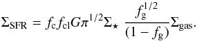$Σ_{SFR} = f_{c} f_{cl} G π^{1 / 2} Σ_{⋆} \frac{f_{g}^{1 / 2}}{(1 - f_{g})} Σ_{gas} .$ $\appendix \setcounter{section}{1} \begin{equation} \Sigma_{\rm SFR} = f_{\rm c} f_{\rm cl} G \pi^{1/2} {\Sigma}_{\star}\ \frac{f_{\rm g}^{1/2}}{(1-f _{\rm g})} \Sigma_{\rm gas}. \label{eqn:SFRder2} \end{equation}$ (A.2)The total SN energy input into the ISM is 10⁵¹ erg, for an assumed canonical supernova energy transfer efficiency into momentum of the ISM of 0.01, and v_c = 400 km s^-1 (Silk & Norman 2009). The relevant quantities for the distribution of the gas, f_c and f_cl, are not well constrained in galaxies, but reasonable numbers are f_c = 0.2 and f_cl = 0.1, and these clouds are mildly over pressurized relative to the ISM ( $\frac{p_{g}}{p_{cl}}$ $\hbox{${p_{\rm g}}\over{p_{\rm cl}}$}$ is approximately a few; where we have chosen 2).

To derive the final version of the relationship (Eq. (1)), we simply multiplied Eq. (A.2) by the disk area (i.e., SFR = 2πr $\begin{matrix} 2 \\ e \end{matrix}$ $\hbox{$_{\rm e}^2$}$ Σ_SFR and M_⋆ = 2π r $\begin{matrix} 2 \\ e \end{matrix}$ $\hbox{$_{\rm e}^2$}$ Σ_⋆). Thus we assumed that the area covered by star formation is that of the stellar disk, which of course is the fundamental assumption in a generalized Schmidt law.

All Figures

Fig. 1

Star formation rate (SFR, in M_⊙ yr^-1) as function of total stellar mass (M_⋆, in M_⊙) in two galaxy samples. The data points are estimates of the star formation rate and stellar mass for samples of galaxies at z ~ 1 (blue circles; Elbaz et al. 2007) and z ~ 2 (red circles; Daddi et al. 2007). The green and purple solid lines indicate the best fits to the data sets at z ~ 1 and z ~ 2 from the original papers. The two red lines indicate our simple star formation model with the best scaling parameters adopted (see text for details).

In the text

Fig. 2

Specific star formation rate (sSFR, in Gyr^-1) as a function of redshift. The various points represent measurements from the literature at M_⋆ ~ 10¹⁰M_⊙; see the references in the legend at the bottom right. We note that we have specifically shown the determinations from (Stark et al. 2013) with their uncertainties (red squares) because there is some controversy as to whether or not there is any evolution in the sSFR with increasing redshift beyond z = 2. Since the slope of the sSFR − M_⋆ relation is approximately zero, the rate at which the sSFR evolves is largely independent of M_⋆, except at the highest masses. The lines represent the best-fit relation from Elbaz et al. (2011) over the redshift range 0 to 2 (blue line) and a simple scenario, sSFR (z) = (1 + z)³/t_H0 (where t_H0 is the Hubble time at z = 0, red line), and the blue squares are the estimates for our hypothesis relating the turbulence to the star formation intensity (see text for details). The blue shaded region represents the scatter in the observed sSFR values (±0.3 dex). This rendition of the evolution of the sSFR is inspired by a similar plot in Weinmann et al. (2011).

In the text

Fig. 3

Star formation intensity (Σ_SFR, in M_⊙ yr^-1 kpc^-2) as a function of redshift. The evolution of the generalized Schmidt law (black line) compared to the evolution of abudance-matched star-forming galaxies (i.e., galaxies with co-moving number densities like that of MW mass galaxies in the local Universe) for several types of size evolution (r_e = 3.6(M_⋆/ 5.0 × 10¹⁰)^0.27 – solid red line; r_e = 3.6(1. + z)^-0.55 – upper red dashed line; r_e = 3.6 kpc – lower dashed red line; see van Dokkum et al. 2013, for details). We also show the evolution of the star formation intensity for high redshift galaxies with an sSFR = 2 Gyr^-1, a stellar mass of 5 × 10⁹M_⊙, and a size evolution, r_e = 2.5((1 + z)/3)^-1.2 kpc (blue line and shaded region representing a scatter of ±0.3 dex; see Oesch et al. 2010; Mosleh et al. 2012). The evolution of the stellar mass surface density, Σ_⋆ (M_⊙ kpc^-2; right hand ordinate) of MW-like galaxies (black dashed line) is a factor of about 3 but includes the growth of the bulge as well as the disk (van Dokkum et al. 2013). We also indicate (dotted line) the star formation intensity threshold for local starburst galaxies to drive winds and indicated the possible range of thresholds from local and distant galaxies (Lehnert & Heckman 1996; Heckman 2003; Le Tiran et al. 2011b; Newman et al. 2012a).

In the text

Fig. 4

Specific star formation rate (sSFR, in Gyr^-1) as a function of the stellar mass surface density (Σ_⋆, in M_⊙ pc^-2) as predicted by a simple relation where the hydrostatic pressure and the thrust of the mechanical energy generated by intense star formation are equal. To span a range of possible sSFR in such a scenario, we vary the input values of the gas fraction, f_g, or the velocity dispersion ratio of the gas and the stars, σ_gas/σ_stars. The red solid lines represent this equality for a range of gas fractions, f_g = 0.3 to 0.7, and for a constant σ_gas/σ_stars = 1, while the blue lines represent this equality for a constant gas fraction, f_g = 0.3, and a range of σ_gas/σ_stars = 0.25−1.25 in steps of 0.25. The hatched regions indicate approximately the observed range of stellar mass surface densities and sSFR at z ~ 2 (diagonally hatched region) and z ~ 5−7 (cross-hatched region; see text for details).

In the text

Fig. 5

Specific star formation rate (sSFR, in Gyr^-1) as a function of stellar mass surface density (Σ_⋆, in M_⊙ pc^-2), for the hypothesis that the star formation drives galaxies towards the line of stability against star formation (Toomre parameter, Q = 1) as described in the text. The red and blue solid lines represents the sSFR where the energy input from massive stars generates enough turbulence to drive the global ISM towards Q ~ 1. The red solid lines represent where Q ~ 1 for a range of gas fractions (f_g = 0.3 to 0.7) and for a constant σ_gas/σ_stars = 1, while the blue lines represent where Q = 1 for a constant gas fraction (f_g = 0.5) and σ_gas/σ_stars = 1, but now for a range of energy input from massive stars into the turbulence of the ISM, ϵ = 100–160 km s^-1 kpc yr $^{1 / 2} M_{⊙}^{- 1 / 2}$ $\hbox{$^{1/2}~M_{\sun}^{-1/2}$}$ , where ϵ is the coupling between the star formation intensity and the velocity dispersion (Lehnert et al. 2009, 2013). The predicted sSFR values increase with increasing gas fraction but decrease with increasing ϵ. The hatched regions are the same as in Fig. 4.

In the text

Current usage metrics show cumulative count of Article Views (full-text article views including HTML views, PDF and ePub downloads, according to the available data) and Abstracts Views on Vision4Press platform.

Data correspond to usage on the plateform after 2015. The current usage metrics is available 48-96 hours after online publication and is updated daily on week days.

Initial download of the metrics may take a while.

[1] Abramson, L. E., Kelson, D. D., Dressler, A., et al. 2014, ApJ, 785, L36 [NASA ADS] [CrossRef] [Google Scholar]

[2] Agertz, O., Lake, G., Teyssier, R., et al. 2009, MNRAS, 392, 294 [NASA ADS] [CrossRef] [Google Scholar]

[3] Aravena, M., Carilli, C., Daddi, E., et al. 2010, ApJ, 718, 177 [NASA ADS] [CrossRef] [Google Scholar]

[4] Baldry, I. K., Glazebrook, K., & Driver, S. P. 2008, MNRAS, 388, 945 [NASA ADS] [Google Scholar]

[5] Barden, M., Rix, H.-W., Somerville, R. S., et al. 2005, ApJ, 635, 959 [NASA ADS] [CrossRef] [Google Scholar]

[6] Barker, M. K., Ferguson, A. M. N., Cole, A. A., et al. 2011, MNRAS, 410, 504 [NASA ADS] [CrossRef] [Google Scholar]

[7] Behroozi, P. S., Wechsler, R. H., & Conroy, C. 2013, ApJ, 770, 57 [NASA ADS] [CrossRef] [Google Scholar]

[8] Bernardi, M., Shankar, F., Hyde, J. B., et al. 2010, MNRAS, 404, 2087 [NASA ADS] [Google Scholar]

[9] Bigiel, F., & Blitz, L. 2012, ApJ, 756, 183 [NASA ADS] [CrossRef] [Google Scholar]

[10] Bigiel, F., Leroy, A., Walter, F., et al. 2010, AJ, 140, 1194 [NASA ADS] [CrossRef] [Google Scholar]

[11] Bird, J. C., Kazantzidis, S., Weinberg, D. H., et al. 2013, ApJ, 773, 43 [NASA ADS] [CrossRef] [MathSciNet] [Google Scholar]

[12] Birnboim, Y., & Balberg, S. 2013, ArXiv e-prints [arXiv:1311.1206] [Google Scholar]

[13] Blitz, L., & Rosolowsky, E. 2006, ApJ, 650, 933 [NASA ADS] [CrossRef] [Google Scholar]

[14] Bond, N. A., Ivezić, Ž., Sesar, B., et al. 2010, ApJ, 716, 1 [NASA ADS] [CrossRef] [Google Scholar]

[15] Bottema, R. 1993, A&A, 275, 16 [NASA ADS] [Google Scholar]

[16] Bouché, N., Cresci, G., Davies, R., et al. 2007, ApJ, 671, 303 [NASA ADS] [CrossRef] [Google Scholar]

[17] Bouché, N., Dekel, A., Genzel, R., et al. 2010, ApJ, 718, 1001 [NASA ADS] [CrossRef] [Google Scholar]

[18] Bouché, N., Hohensee, W., Vargas, R., et al. 2012, MNRAS, 426, 801 [NASA ADS] [CrossRef] [Google Scholar]

[19] Bovy, J., Rix, H.-W., Hogg, D. W., et al. 2012, ApJ, 755, 115 [NASA ADS] [CrossRef] [Google Scholar]

[20] Brook, C. B., Stinson, G. S., Gibson, B. K., et al. 2012, MNRAS, 426, 690 [NASA ADS] [CrossRef] [Google Scholar]

[21] Carollo, C. M., Bschorr, T. J., Renzini, A., et al. 2013, ApJ, 773, 112 [NASA ADS] [CrossRef] [Google Scholar]

[22] Ceverino, D., Dekel, A., Mandelker, N., et al. 2012, MNRAS, 420, 3490 [NASA ADS] [CrossRef] [Google Scholar]

[23] Chiappini, C., Renda, A., & Matteucci, F. 2002, A&A, 395, 789 [NASA ADS] [CrossRef] [EDP Sciences] [Google Scholar]

[24] Codis, S., Pichon, C., Devriendt, J., et al. 2012, MNRAS, 427, 3320 [NASA ADS] [CrossRef] [Google Scholar]

[25] Coil, A. L., Weiner, B. J., Holz, D. E., et al. 2011, ApJ, 743, 46 [NASA ADS] [CrossRef] [Google Scholar]

[26] Daddi, E., Dickinson, M., Morrison, G., et al. 2007, ApJ, 670, 156 [NASA ADS] [CrossRef] [Google Scholar]

[27] Daddi, E., Dannerbauer, H., Krips, M., et al. 2009, ApJ, 695, L176 [NASA ADS] [CrossRef] [Google Scholar]

[28] Daddi, E., Bournaud, F., Walter, F., et al. 2010, ApJ, 713, 686 [NASA ADS] [CrossRef] [Google Scholar]

[29] Dannerbauer, H., Daddi, E., Riechers, D. A., et al. 2009, ApJ, 698, L178 [NASA ADS] [CrossRef] [Google Scholar]

[30] Danovich, M., Dekel, A., Hahn, O., Ceverino, D., & Primack, J. 2015, MNRAS, 449, 2087 [NASA ADS] [CrossRef] [Google Scholar]

[31] Davé, R., Oppenheimer, B. D., & Finlator, K. 2011, MNRAS, 415, 11 [NASA ADS] [CrossRef] [Google Scholar]

[32] Davies, L. J. M., Bremer, M. N., Stanway, E. R., et al. 2012, MNRAS, 425, 153 [NASA ADS] [CrossRef] [Google Scholar]

[33] Dekel, A., Sari, R., & Ceverino, D. 2009, ApJ, 703, 785 [Google Scholar]

[34] Dekel, A., Zolotov, A., Tweed, D., et al. 2013, MNRAS, 435, 999 [NASA ADS] [CrossRef] [Google Scholar]

[35] Dopita, M. A., & Ryder, S. D. 1994, ApJ, 430, 163 [NASA ADS] [CrossRef] [Google Scholar]

[36] Dubois, Y., Pichon, C., Devriendt, J., et al. 2013, MNRAS, 428, 2885 [NASA ADS] [CrossRef] [Google Scholar]

[37] Dunne, L., Ivison, R. J., Maddox, S., et al. 2009, MNRAS, 394, 3 [NASA ADS] [CrossRef] [Google Scholar]

[38] Dutton, A. A., van den Bosch, F. C., & Dekel, A. 2010, MNRAS, 405, 1690 [NASA ADS] [Google Scholar]

[39] Elbaz, D., Daddi, E., Le Borgne, D., et al. 2007, A&A, 468, 33 [NASA ADS] [CrossRef] [EDP Sciences] [Google Scholar]

[40] Elbaz, D., Dickinson, M., Hwang, H. S., et al. 2011, A&A, 533, A119 [NASA ADS] [CrossRef] [EDP Sciences] [Google Scholar]

[41] Elmegreen, B. G. 1989, ApJ, 338, 178 [NASA ADS] [CrossRef] [Google Scholar]

[42] Elmegreen, B. G. 1993, ApJ, 411, 170 [NASA ADS] [CrossRef] [Google Scholar]

[43] Elmegreen, D. M., & Elmegreen, B. G. 2006, ApJ, 651, 676 [NASA ADS] [CrossRef] [Google Scholar]

[44] Elmegreen, B. G., Elmegreen, D. M., Fernandez, M. X., & Lemonias, J. J. 2009a, ApJ, 692, 12 [NASA ADS] [CrossRef] [Google Scholar]

[45] Elmegreen, D. M., Elmegreen, B. G., Marcus, M. T., et al. 2009b, ApJ, 701, 306 [NASA ADS] [CrossRef] [Google Scholar]

[46] Epinat, B., Contini, T., Le Fèvre, O., et al. 2009, A&A, 504, 789 [NASA ADS] [CrossRef] [EDP Sciences] [Google Scholar]

[47] Epinat, B., Amram, P., Balkowski, C., & Marcelin, M. 2010, MNRAS, 401, 2113 [NASA ADS] [CrossRef] [Google Scholar]

[48] Fathi, K., Allen, M., Boch, T., Hatziminaoglou, E., & Peletier, R. F. 2010, MNRAS, 406, 1595 [NASA ADS] [Google Scholar]

[49] Feldmann, R. 2013, MNRAS, 433, 1910 [NASA ADS] [CrossRef] [Google Scholar]

[50] Feldmann, R., Hernandez, J., & Gnedin, N. Y. 2012, ApJ, 761, 167 [NASA ADS] [CrossRef] [Google Scholar]

[51] Ferguson, A. M. N., & Johnson, R. A. 2001, ApJ, 559, L13 [NASA ADS] [CrossRef] [Google Scholar]

[52] Feulner, G., Gabasch, A., Salvato, M., et al. 2005, ApJ, 633, L9 [NASA ADS] [CrossRef] [Google Scholar]

[53] Förster Schreiber, N. M., Genzel, R., Bouché, N., et al. 2009, ApJ, 706, 1364 [NASA ADS] [CrossRef] [Google Scholar]

[54] Förster Schreiber, N. M., Shapley, A. E., Erb, D. K., et al. 2011, ApJ, 731, 65 [NASA ADS] [CrossRef] [Google Scholar]

[55] Guo, Y., Giavalisco, M., Ferguson, H. C., Cassata, P., & Koekemoer, A. M. 2012, ApJ, 757, 120 [NASA ADS] [CrossRef] [Google Scholar]

[56] Haywood, M. 2001, MNRAS, 325, 1365 [NASA ADS] [CrossRef] [Google Scholar]

[57] Haywood, M., Di Matteo, P., Lehnert, M. D., Katz, D., & Gómez, A. 2013, A&A, 560, A109 [NASA ADS] [CrossRef] [EDP Sciences] [Google Scholar]

[58] Heckman, T. M. 2003, Rev. Mex. Astron. Astrofis. Conf. Ser., 17, 47 [Google Scholar]

[59] Heckman, T. M., Armus, L., & Miley, G. K. 1990, ApJS, 74, 833 [NASA ADS] [CrossRef] [Google Scholar]

[60] Hernandez, X., Valls-Gabaud, D., & Gilmore, G. 2000, MNRAS, 316, 605 [NASA ADS] [CrossRef] [Google Scholar]

[61] Hopkins, P. F., Kereš, D., & Murray, N. 2013, MNRAS, 432, 2639 [NASA ADS] [CrossRef] [Google Scholar]

[62] Inoue, T., & Fukui, Y. 2013, ApJ, 774, L31 [NASA ADS] [CrossRef] [Google Scholar]

[63] Johansson, J., Thomas, D., & Maraston, C. 2012, MNRAS, 421, 1908 [NASA ADS] [CrossRef] [Google Scholar]

[64] Jurić, M., Ivezić, Ž., Brooks, A., et al. 2008, ApJ, 673, 864 [NASA ADS] [CrossRef] [MathSciNet] [Google Scholar]

[65] Kang, X., Lin, W. P., Skibba, R., & Chen, D. N. 2010, ApJ, 713, 1301 [NASA ADS] [CrossRef] [Google Scholar]

[66] Karim, A., Schinnerer, E., Martínez-Sansigre, A., et al. 2011, ApJ, 730, 61 [NASA ADS] [CrossRef] [Google Scholar]

[67] Kassin, S. A., Weiner, B. J., Faber, S. M., et al. 2012, ApJ, 758, 106 [NASA ADS] [CrossRef] [Google Scholar]

[68] Khochfar, S., & Silk, J. 2011, MNRAS, 410, L42 [NASA ADS] [Google Scholar]

[69] Lagarde, N., Romano, D., Charbonnel, C., et al. 2012, A&A, 542, A62 [NASA ADS] [CrossRef] [EDP Sciences] [Google Scholar]

[70] Lagos, C. D. P., Lacey, C. G., & Baugh, C. M. 2013, MNRAS, 436, 1787 [NASA ADS] [CrossRef] [Google Scholar]

[71] Lara-López, M. A., Hopkins, A. M., López-Sánchez, A. R., et al. 2013, MNRAS, 434, 451 [NASA ADS] [CrossRef] [Google Scholar]

[72] Law, D. R., Steidel, C. C., Erb, D. K., et al. 2009, ApJ, 697, 2057 [NASA ADS] [CrossRef] [Google Scholar]

[73] Le Tiran, L., Lehnert, M. D., Di Matteo, P., Nesvadba, N. P. H., & van Driel, W. 2011a, A&A, 530, L6 [NASA ADS] [CrossRef] [EDP Sciences] [Google Scholar]

[74] Le Tiran, L., Lehnert, M. D., van Driel, W., Nesvadba, N. P. H., & Di Matteo, P. 2011b, A&A, 534, L4 [NASA ADS] [CrossRef] [EDP Sciences] [Google Scholar]

[75] Lehnert, M. D., & Heckman, T. M. 1996, ApJ, 462, 651 [NASA ADS] [CrossRef] [Google Scholar]

[76] Lehnert, M. D., Nesvadba, N. P. H., Tiran, L. L., et al. 2009, ApJ, 699, 1660 [NASA ADS] [CrossRef] [Google Scholar]

[77] Lehnert, M. D., Le Tiran, L., Nesvadba, N. P. H., et al. 2013, A&A, 555, A72 [NASA ADS] [CrossRef] [EDP Sciences] [Google Scholar]

[78] Lehnert, M. D., Di Matteo, P., Haywood, M., & Snaith, O. N. 2014, ApJ, 789, L30 [NASA ADS] [CrossRef] [Google Scholar]

[79] Leitherer, C., Schaerer, D., Goldader, J. D., et al. 1999, ApJS, 123, 3 [NASA ADS] [CrossRef] [Google Scholar]

[80] Leitner, S. N. 2012, ApJ, 745, 149 [NASA ADS] [CrossRef] [Google Scholar]

[81] Leitner, S. N., & Kravtsov, A. V. 2011, ApJ, 734, 48 [NASA ADS] [CrossRef] [Google Scholar]

[82] Leroy, A. K., Walter, F., Brinks, E., et al. 2008, AJ, 136, 2782 [NASA ADS] [CrossRef] [Google Scholar]

[83] Leroy, A. K., Walter, F., Sandstrom, K., et al. 2013, AJ, 146, 19 [NASA ADS] [CrossRef] [Google Scholar]

[84] Lilly, S. J., Carollo, C. M., Pipino, A., Renzini, A., & Peng, Y. 2013, ApJ, 772, 119 [NASA ADS] [CrossRef] [Google Scholar]

[85] Magdis, G. E., Elbaz, D., Daddi, E., et al. 2010, ApJ, 714, 1740 [NASA ADS] [CrossRef] [Google Scholar]

[86] Martig, M., & Bournaud, F. 2010, ApJ, 714, L275 [NASA ADS] [CrossRef] [Google Scholar]

[87] Martin, C. L., Shapley, A. E., Coil, A. L., et al. 2012, ApJ, 760, 127 [NASA ADS] [CrossRef] [Google Scholar]

[88] Masset, F., & Tagger, M. 1997, A&A, 322, 442 [NASA ADS] [Google Scholar]

[89] Mo, H. J., Mao, S., & White, S. D. M. 1998, MNRAS, 295, 319 [Google Scholar]

[90] Moran, E. C., Lehnert, M. D., & Helfand, D. J. 1999, ApJ, 526, 649 [NASA ADS] [CrossRef] [Google Scholar]

[91] Mosleh, M., Williams, R. J., Franx, M., & Kriek, M. 2011, ApJ, 727, 5 [NASA ADS] [CrossRef] [Google Scholar]

[92] Mosleh, M., Williams, R. J., Franx, M., et al. 2012, ApJ, 756, L12 [NASA ADS] [CrossRef] [Google Scholar]

[93] Neistein, E., & Dekel, A. 2008, MNRAS, 388, 1792 [NASA ADS] [CrossRef] [Google Scholar]

[94] Neistein, E., Maoz, D., Rix, H.-W., & Tonry, J. L. 1999, AJ, 117, 2666 [NASA ADS] [CrossRef] [Google Scholar]

[95] Newman, S. F., Genzel, R., Förster-Schreiber, N. M., et al. 2012a, ApJ, 761, 43 [NASA ADS] [CrossRef] [Google Scholar]

[96] Newman, S. F., Shapiro Griffin, K., Genzel, R., et al. 2012b, ApJ, 752, 111 [NASA ADS] [CrossRef] [Google Scholar]

[97] Noeske, K. G., Weiner, B. J., Faber, S. M., et al. 2007, ApJ, 660, L43 [Google Scholar]

[98] Oesch, P. A., Bouwens, R. J., Carollo, C. M., et al. 2010, ApJ, 709, L21 [NASA ADS] [CrossRef] [Google Scholar]

[99] Oliver, S., Frost, M., Farrah, D., et al. 2010, MNRAS, 405, 2279 [NASA ADS] [Google Scholar]

[100] Papastergis, E., Cattaneo, A., Huang, S., Giovanelli, R., & Haynes, M. P. 2012, ApJ, 759, 138 [NASA ADS] [CrossRef] [Google Scholar]

[101] Peirani, S., Jung, I., Silk, J., & Pichon, C. 2012, MNRAS, 427, 2625 [NASA ADS] [CrossRef] [Google Scholar]

[102] Pichon, C., Pogosyan, D., Kimm, T., et al. 2011, MNRAS, 418, 2493 [NASA ADS] [CrossRef] [Google Scholar]

[103] Prodanović, T., Steigman, G., & Fields, B. D. 2010, MNRAS, 406, 1108 [NASA ADS] [Google Scholar]

[104] Qu, Y., Di Matteo, P., Lehnert, M. D., van Driel, W., & Jog, C. J. 2011, A&A, 535, A5 [NASA ADS] [CrossRef] [EDP Sciences] [Google Scholar]

[105] Renaud, F., Kraljic, K., & Bournaud, F. 2012, ApJ, 760, L16 [NASA ADS] [CrossRef] [Google Scholar]

[106] Rodighiero, G., Vaccari, M., Franceschini, A., et al. 2010, A&A, 515, A8 [NASA ADS] [CrossRef] [EDP Sciences] [Google Scholar]

[107] Romano, D., Tosi, M., Chiappini, C., & Matteucci, F. 2006, MNRAS, 369, 295 [NASA ADS] [CrossRef] [Google Scholar]

[108] Rubin, K. H. R., Weiner, B. J., Koo, D. C., et al. 2010, ApJ, 719, 1503 [NASA ADS] [CrossRef] [Google Scholar]

[109] Rubin, K. H. R., Prochaska, J. X., Koo, D. C., et al. 2014, ApJ, 794, 156 [NASA ADS] [CrossRef] [Google Scholar]

[110] Salmi, F., Daddi, E., Elbaz, D., et al. 2012, ApJ, 754, L14 [NASA ADS] [CrossRef] [Google Scholar]

[111] Schruba, A., Leroy, A. K., Walter, F., et al. 2011, AJ, 142, 37 [NASA ADS] [CrossRef] [Google Scholar]

[112] Shen, S., Mo, H. J., White, S. D. M., et al. 2003, MNRAS, 343, 978 [NASA ADS] [CrossRef] [Google Scholar]

[113] Shi, Y., Helou, G., Yan, L., et al. 2011, ApJ, 733, 87 [NASA ADS] [CrossRef] [Google Scholar]

[114] Silk, J. 1997, ApJ, 481, 703 [NASA ADS] [CrossRef] [Google Scholar]

[115] Silk, J., & Mamon, G. A. 2012, RA&A, 12, 917 [Google Scholar]

[116] Silk, J., & Norman, C. 2009, ApJ, 700, 262 [NASA ADS] [CrossRef] [Google Scholar]

[117] Snaith, O. N., Haywood, M., Di Matteo, P., et al. 2014, ApJ, 781, L31 [CrossRef] [Google Scholar]

[118] Stark, D. P., Ellis, R. S., Bunker, A., et al. 2009, ApJ, 697, 1493 [NASA ADS] [CrossRef] [Google Scholar]

[119] Stark, D. P., Schenker, M. A., Ellis, R., et al. 2013, ApJ, 763, 129 [NASA ADS] [CrossRef] [Google Scholar]

[120] Steidel, C. C., Erb, D. K., Shapley, A. E., et al. 2010, ApJ, 717, 289 [NASA ADS] [CrossRef] [Google Scholar]

[121] Stewart, K. R., Kaufmann, T., Bullock, J. S., et al. 2011, ApJ, 738, 39 [NASA ADS] [CrossRef] [Google Scholar]

[122] Strickland, D. K., & Heckman, T. M. 2009, ApJ, 697, 2030 [NASA ADS] [CrossRef] [Google Scholar]

[123] Swinbank, A. M., Papadopoulos, P. P., Cox, P., et al. 2011, ApJ, 742, 11 [NASA ADS] [CrossRef] [Google Scholar]

[124] Tacconi, L. J., Genzel, R., Neri, R., et al. 2010, Nature, 463, 781 [Google Scholar]

[125] Tacconi, L. J., Neri, R., Genzel, R., et al. 2013, ApJ, 768, 74 [Google Scholar]

[126] Tamburro, D., Rix, H.-W., Leroy, A. K., et al. 2009, AJ, 137, 4424 [NASA ADS] [CrossRef] [Google Scholar]

[127] van Dokkum, P. G., Leja, J., Nelson, E. J., et al. 2013, ApJ, 771, L35 [NASA ADS] [CrossRef] [Google Scholar]

[128] Verma, A., Lehnert, M. D., Förster Schreiber, N. M., Bremer, M. N., & Douglas, L. 2007, MNRAS, 377, 1024 [NASA ADS] [CrossRef] [Google Scholar]

[129] Vlajić, M., Bland-Hawthorn, J., & Freeman, K. C. 2009, ApJ, 697, 361 [NASA ADS] [CrossRef] [Google Scholar]

[130] Wang, B., & Silk, J. 1994, ApJ, 427, 759 [NASA ADS] [CrossRef] [Google Scholar]

[131] Weiner, B. J., Coil, A. L., Prochaska, J. X., et al. 2009, ApJ, 692, 187 [NASA ADS] [CrossRef] [Google Scholar]

[132] Weinmann, S. M., Neistein, E., & Dekel, A. 2011, MNRAS, 417, 2737 [NASA ADS] [CrossRef] [Google Scholar]

[133] Weinmann, S. M., Franx, M., van Dokkum, P., & Bezanson, R. 2013, ApJ, 767, L21 [NASA ADS] [CrossRef] [Google Scholar]

[134] Wilson, C. D., Warren, B. E., Irwin, J., et al. 2011, MNRAS, 410, 1409 [NASA ADS] [Google Scholar]

[135] Wolfire, M. G., Hollenbach, D., McKee, C. F., Tielens, A. G. G. M., & Bakes, E. L. O. 1995, ApJ, 443, 152 [Google Scholar]

[136] Wuyts, S., Förster Schreiber, N. M., van der Wel, A., et al. 2011, ApJ, 742, 96 [NASA ADS] [CrossRef] [Google Scholar]

[137] Wyithe, J. S. B., Loeb, A., & Oesch, P. A. 2014, MNRAS, 439, 1326 [NASA ADS] [CrossRef] [Google Scholar]

[138] Young, J. S., & Knezek, P. M. 1989, ApJ, 347, L55 [NASA ADS] [CrossRef] [Google Scholar]

[139] Young, J. S., Xie, S., Tacconi, L., et al. 1995, ApJS, 98, 219 [NASA ADS] [CrossRef] [Google Scholar]

[140] Yuma, S., Ohta, K., Yabe, K., Kajisawa, M., & Ichikawa, T. 2011, ApJ, 736, 92 [NASA ADS] [CrossRef] [Google Scholar]

[141] Zhang, L., Rix, H.-W., van de Ven, G., et al. 2013, ApJ, 772, 108 [NASA ADS] [CrossRef] [Google Scholar]

On the cosmic evolution of the specific star formation rate

1. Introduction

2. The ridge line in the SFR – M⋆ plane

2.1. A simple model relating overall SFR to ISM pressure

2.2. Choices made for this model

2.2.1. Exponents in the generalized Schmidt law, m + n = 2

2.2.2. Exponents in the generalized Schmidt law, m + n ≲ 2

2.2.3. Equal velocity dispersions of gas and stars

2.2.4. A constant efficiency factor in the generalized Schmidt law

3. Cosmic evolution of the sSFR

3.1. The evolution of angular momentum

3.2. The declining sSFR at z ≲ 2

3.2.1. The importance of mass return

3.2.2. Why the break in the sSFR evolution at z ~ 2?

3.3. Mechanical and radiative self-regulated star formation

3.3.1. Wind and radiative thrust balancing hydrostatic pressure

3.3.2. Turbulent pressure and the line of stability (Q ~ 1)

3.3.3. Comparison with other sSFR evolution models

4. Summary

Acknowledgments

References

Appendix A: On Eq. (1)

All Figures

2. The ridge line in the SFR – M_⋆ plane