| Issue |
A&A
Volume 576, April 2015
|
|
|---|---|---|
| Article Number | A54 | |
| Number of page(s) | 6 | |
| Section | The Sun | |
| DOI | https://doi.org/10.1051/0004-6361/201425116 | |
| Published online | 27 March 2015 | |
Short-term variability of inner-source pickup ions at 1 AU
SOHO/CELIAS observations
Institut für Experimentelle und Angewandte Physik (IEAP), Christian
Albrechts-Universität zu Kiel,
Leibnizstrasse 11,
24118
Kiel,
Germany
e-mail:
berger@physik.uni-kiel.de
Received: 6 October 2014
Accepted: 30 January 2015
Context. In 1995 a second extended source of pickup ions in the inner heliosphere was discovered. Since then this so-called inner source has been characterised in many studies, and various scenarios for its nature have been proposed. But to this day, the detailed nature of the inner source is still unknown.
Aims. Although it seems most likely that an interaction of solar wind and dust plays a key role in the production of the inner source pickup ions, available observations have not provided conclusive evidence for any proposed scenario. By analysing the short-term variability of the inner source, we determine a new observational constraint to address the nature of the inner source.
Methods. We used the data set of the charge time-of-flight instrument that operated in 1996 on-board the solar and heliospheric observatory at the first Lagrangian point to analyse inner source O+ and C+. The unmatched combination of mass per charge resolution, which is sufficient to definitely resolve O+ and C+, and typical high count rates of about 150 counts per day allowed us to address the short-term variability of the inner source for the first time.
Results. The comparison of the variability of inner-source and solar-wind ions shows that the flux of inner source pickup oxygen and carbon is directly correlated with the flux of solar wind oxygen, and carbon, respectively.
Conclusions. Among the scenarios for the nature of the inner source alone, the scenario of solar-wind neutralisation agrees with this new observational constraint.
Key words: solar wind / interplanetary medium
© ESO, 2015
1. Introduction
Observations in the inner heliosphere have shown that there are two extended sources for the production of pickup ions (PUIs). The first source has been unambigiously identified as interstellar neutral atoms that can penetrate deep into the heliosphere unimpeded by electro-magnetic forces. In fact the existence and the nature of this interstellar source was predicted (Fahr 1974) prior to its first observation (Moebius et al. 1985). The advent of the idea of a second so-called inner source had been marked ten years after the first observation of interstellar pickup He+ by the discovery of one-fold ionised carbon that could not be attributed to the interstellar source (Geiss et al. 1995).
The inner source has been analysed in many subsequent studies and several characteristics have been inferred from the results. Direct observed characteristics are that it resembles the solar wind composition (Gloeckler et al. 2000), is randomly distributed (Geiss et al. 1996), produces a large continous flux (Geiss et al. 1996), and is stable over the solar cycle (Allegrini et al. 2005). There is also evidence of a correlation of solar-wind H+ and inner-source PUI flux (Allegrini et al. 2005).
Another characteristic, a peak production close to the Sun within 10 to 30 solar radii, has been deduced from the shape of observed velocity spectra (Schwadron et al. 2000). However, this last characteristic depends on assumptions about the nature of the inner source, for which various scenarios have been proposed (Gloeckler et al. 2000; Schwadron et al. 2000; Wimmer-Schweingruber & Bochsler 2003; Bzowski & Krolikowska 2005; Mann & Czechowski 2005). All settings assume that dust is important for generating the inner-source pickup ions, but so far none agrees with all observational constraints (Allegrini et al. 2005). Nevertheless, the observations are suggestive of a direct involvement of solar wind ions in the inner-source PUI production mechanism. Among them all, the two scenarios assuming an interaction of solar wind and dust are the most likely ones. The first proposed mechanism is called solar-wind recycling. Solar wind is implanted in and subsequently released by large μm dust grains close to the Sun (Gloeckler et al. 2000; Schwadron et al. 2000). In the second mechanism, called solar-wind neutralisation, solar wind is neutralised on penetration of small nm size dust grains (Wimmer-Schweingruber & Bochsler 2003). This scenario does not require a peak of production close to the Sun (Bochsler et al. 2006, 2007).
Despite the progress that has been made in the past two decades, existing dust and pickup ion measurements have not been sufficient to pinpoint the nature of the inner source conclusively (Allegrini et al. 2005). Inner source PUIs are hard to observe, because their flux is several orders of magnitude lower than the bulk solar wind flux. Previous studies using the Solar Wind Ion Composition Spectrometer (SWICS) on Ulysses measured approximately a single C+ ion per day. For example, the study of the stability over the solar cycle by Allegrini et al. (2005), comparing three periods of about 64 days each, was based on a total of ~200 C+ counts. Consequently, the short-term behaviour of the inner source has not been accessible and is unknown to this day.
For this reason, the Charge Time Of Flight instrument (CTOF) which operated in 1996 as part of the Charge, Element, and Isotope Analysis System (CELIAS; Hovestadt et al. 1995) on the SOlar Heliospheric Observatory (SOHO) is perfectly suited to studying inner-source PUIs (Berger et al. 2012). O+ and C+ are clearly resolved, and the count rates exceed previous studies by more than two orders of magnitude. Surprisingly, the data, with one exception of Venus tail ray O+ observations (Grünwaldt et al. 1997), has never been used to study inner source PUIs, although CTOFs active phase coincides with the discovery of the inner source. In this work and a companion paper (Taut et al. 2015) we investigate inner source PUIs using CTOF data. Here, we address the short-term variability of inner source O+ and C+ while the companion paper adresses the composition of the inner source.
2. Method
The difference in the two production mechanisms of solar-wind recycling and solar-wind neutralisation is likely to affect the in-situ short-term behaviour of the inner source. Thus, it provides an additional observational constraint for distinguishing between the two scenarios. Arising from the two-step nature of the production mechanism in the solar-wind recycling scenario, there should be a phase shift between solar-wind heavy-ion flux and inner-source PUI flux. An implanted ion remains in the grain for a certain time τ until it is relased by grain sputtering caused by the total solar-wind flux. This time can be estimated as τ(r) = λ/S(r) (Wimmer-Schweingruber & Bochsler 2003). Using a typical implantation depth λ ≥ 100 Å and a grain sputtering rate S(1 AU)= 1 Å yr-1, we get τ(0.05 AU) ≥ 0.25 yr for the expected position of the peak production at r = 0.05 AU. In the case of the solar-wind neutralisation scenario, the production is nearly instantaneous, so for neutralisation, we expect the variability of an inner source PUI species to correlate with the corresponding solar wind flux of its element; for example, the variability of O+ should be correlated with the variability of the total solar wind oxygen flux. For the recycling scenario, with τ(0.05 AU) ≥ 0.25 yr, even slow solar wind with vsw = 300 km s-1 has covered a distance of more than 15 AU, and the in-situ flux of inner source PUIs should be uncorrelated with the solar-wind flux of the same element. Instead we expect a correlation of the variability of all inner source PUI species with the solar-wind proton flux that is the main driver for grain sputtering. Investigating the correlation of inner-source and solar-wind ions allows us to identifiy the most likely candidate for the production scenario of the inner source.
3. Observations and analysis technique
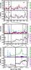 |
Fig. 1 Time series of CTOF count rates for inner-source C+ and O+, and solar-wind O6+ (upper sub-panels) and PM solar-wind speed and flux vsw and fsw (lower sub-panels) are shown for daily, hourly, and 5-min cadences (top, middle, bottom panel). |
To study the short-term variability of inner-source pickup ions we used observations from SOHO/CELIAS that were obtained in the period from days 150 to 220 in 1996. For this period data from CTOF and the Proton Monitor (PM), which are both part of CELIAS, are available, and fluxes of solar-wind protons and O6+ can be compared to pickup He+, O+, and C+. Solar wind (proton) velocity, vsw, and proton density, nsw, and thus proton flux, fsw, are routinely measured by the PM and provided via the SOHO archive in five-minute resolution. The remaining ions have been observed by CTOF. In the case of solar wind O6+, CTOF matrix rate data were analysed according to Hefti (1997) to determine five-minute count rates. For the pickup ions, we analysed CTOF pulse-height analysis data and extracted velocity spectra with a five-minute cadence according to Berger et al. (2012).
Figure 1 shows a time series of the data products in daily, hourly, and five-minute cadences. We set limits in w = vion/vsw to select inner-source PUIs. The lower limits wO+> 0.8 for O+ and wC+> 1.0 for C+ have been set to avoid the background caused by solar wind iron and pickup helium. Upper limits for O+ and C+ have been set to separate inner from interstellar source contributions. While C+ is attributed solely to the inner source, O+ has a significant contribution from interstellar PUIs at wO+> 1.4 (Berger et al. 2012). Thus the upper limits for C+ and O+ have been set to maximum wC+, which can be observed with CTOF, and wO+< 1.4, respectively. Although the count rates of O+ and C+ are more than three orders of magnitude lower than of solar wind O6+, they are much higher than in previous investigations, where a single count per day is typically observed. A strong variability can be seen even in the highest cadence of five minutes.
The period around day of year (DoY) 166, which is shown in the bottom left-hand panel shows significant spikes in the O+ count rates rising from less than one count per five minutes up to 45 counts per five minutes. These spikes are accompanied by small spikes in C+ but without any distinctive features in vsw, fsw, and O6+. A previous study (Grünwaldt et al. 1997) has identified these spikes as Venus tail rays. The bottom right-hand panel shows a second period around DoY 171 in closeup. A clear signature of a compression region in fsw and O6+ is observed. Interestingly, O+ and C+ also show an increase that roughly coincides with the solar-wind compression. The features in the two closeup periods are also visible in the middle panel in a one-hour cadence. In a one-day cadence displayed in the upper panel, the features that happen on time scales of five minutes up to a few hours are hardly visible. But the daily fluxes of solar wind ions, as well as pickup ions, also show strong variabilty. In the following we address the short-term variabilty of O+ and C+.
3.1. Variabilty
As stated above, a correlation of inner-source PUI and solar-wind proton flux would point towards the solar-wind recycling scenario, while a correlation of inner-source PUI, and the corresponding solar-wind heavy ion flux would favour the solar-wind neutralisation scenario.
We now use the CELIAS data to search for correlations between the fluxes of
H+,O6+,O+, and C+. For that we have to account for instrumental
influences. The detection efficiency may vary strongly depending on the ion species and
within one species on the ion velocity. In general, the detection efficiency increases
with ion velocity. In addition, the highest velocity that can be measured with CTOF
depends on the mass per charge of the observed ion species. While O6+ can be measured up to
vmax =
1580 km s-1, the maximum velocity for O+ is vmax = 645
km s-1. Thus, the
phase-space coverage in terms of w depends on the ion species and solar-wind speed. To
calculate the variability of the different species, we have chosen an approach that
implictly accounts for these effects. For a given solar wind speed, vsw(t) =
VSW, and ion species, the phase space
coverage in terms of w and, especially, the detection efficiency for each w is constant
and independent of time. Thus, we can calculate solar wind speed VSW and ion
species-dependent mean five-minute count rates and use them as expectation values. If
TVSW is the set of periods in which
vsw(t) =
VSW and cion(t) are five-minute
ion count rates, the expected count rate in five minutes is given by  (1)Then the relative
varibility in percent can be calculated by
(1)Then the relative
varibility in percent can be calculated by 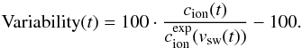 (2)Figure 2 illustrates how the variability of O+ is derived. The upper panels
demonstrate how vsw(t) translates into
(2)Figure 2 illustrates how the variability of O+ is derived. The upper panels
demonstrate how vsw(t) translates into
 ). To get good statistics,
the mean values
). To get good statistics,
the mean values  ) have been calculated
for the whole analysed period from days 150 to 220 and VSW intervals
with widths of 10 km s-1. Because five-minute count rates and expectation values
are too low to get reasonable variabilities using Eq. (2), a temporal binning is applied, and variabilities are derived. The
results for a daily binning are displayed in the lower panels. It can especially be seen
that the deviation between measured and expected counts is typically much greater than the
expected deviations if only counting statistic is assumed (error bars). Therefore, the
derived variabilty can be attributed to a definite temporal variation.
) have been calculated
for the whole analysed period from days 150 to 220 and VSW intervals
with widths of 10 km s-1. Because five-minute count rates and expectation values
are too low to get reasonable variabilities using Eq. (2), a temporal binning is applied, and variabilities are derived. The
results for a daily binning are displayed in the lower panels. It can especially be seen
that the deviation between measured and expected counts is typically much greater than the
expected deviations if only counting statistic is assumed (error bars). Therefore, the
derived variabilty can be attributed to a definite temporal variation.
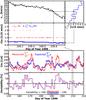 |
Fig. 2 Illustration how O+ daily variabilities are derived. Top main
panel: 5-min solar-wind speeds vsw(t)
(top, left) and expectation values
|
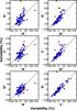 |
Fig. 3 Daily variabilities of various pairs of ions are plotted against each other. The colour indicates values that correspond to certain periods (see Sect. 3.2). |
3.2. Correlations
The calculated variabilities for H+, O6+, O+, and C+ can be compared to search for possible correlations. In the top four panels of Fig. 3 the resulting variabilities for one day temporal binning of C+ and O+ are plotted versus H+ and O6+. It can be seen that inner-source pickup O+ and C+ correlate rather with solar wind O6+ than with solar wind H+. The two bottom panels show the results for O6+ versus H+ and O+ versus C+.
To quantify the correlation for different pairs of ion species the sample correlation coefficient,  , can be calculated. As transient events can strongly influence the obtained variabilities, especially the derived expectation values
  ), we removed such periods from our analysis. First the period around DoY 166 in which venus tail ray O+ is observed (Grünwaldt et al. 1997) must be removed. The strong enhancement of O+ with respect to all other ions, can be seen in the bottom left panel of Fig. 1, and the corresponding variability is marked in green in Fig. 3. Furthermore, the periods DoY 150 to 151 and 183.5 to 184.5, showed an increased proton flux, which is indicated by purple in Fig. 3. Both periods can be attributed to inter-planetary coronal mass ejections (ICMEs; Cane & Richardson 2003). Finally the continous period from DoY 194.5 to 197.5 showed increased fluxes of O+ and C+, indicated by red in Fig. 3. For this period no signature of an ICME has been observed but at approximately DoY 191.5 the Large Angle and Spectrometric COronagraph experiment (LASCO) on SOHO observed a Coronal Mass Ejection (CME) SOHO LASCO CME CATALOG1 (2014) with a large angular extend of 86° and a speed of about 430 km s-1. Because LASCO observations only resolve the CME motion perpendicular to the line of sight, it can not be ruled out that parts of the CME have moved towards SOHO‘s position at the first lagrangian point. If so, its time of arrival would have been in the interval from DoY 194.5 to 197.5. In situ measured vsw around DoY 194.5 rises from ≈315 km s-1 to the derived CME speed of ≈430 km s-1 and stays at velocities above 370 km s-1 until approximately DoY 197.5. Thus, the increased fluxes of O+ and C+ might be related to this CME, although no ICME signatures have been observed in situ. With this we have calculated for two periods, T1 and T2. In T1 only the interval of Venus Tail Ray oberservations (green) has been neglected, wheras in T2 also the periods marked in purple and red have been excluded. Variabilities were calculated for various cadences from 0.1 to 3.0 days in 0.1 steps. The results for T2 are displayed in Fig. 4. In Table 1 the mean value and the standard deviation of for T1 and T2 are given.
Because H+ measurements come from the PM while the remaining ions are measured by CTOF we used CTOF measurements of interstellar pickup He+ in the range 1.5 <wHe+< 2.0 to check whether the good correlation among O6+ and O+, O6+ and C+, and O+ and C+ respectively, might be produced by instrumental effects that have not been considered correctly in our analysis. Therefor, CTOF pulse height analysis data have been analysed and He+ variabilities have been determined similarly as described for C+ and O+. Because  is significantly smaller than
  we can rule out that high values of
  ,
,  , and
, and  are due to instrumental biases.
Mean correlation coefficients (ion2 = row, ion1 = column), and their standard deviations for the two periods T1 and T2 are given.
4. Discussion
Although the correlation coefficient cannot provide definite proof of a causal relationship of the correlated quantities, our results can be interpreted in the context of the two discussed scenarios for the production of inner-source PUIs. In Sect. 2 it was pointed out that a correlation of O+ and solar-wind oxygen would be expected for the solar-wind neutralisation scenario, while a correlation of O+ and solar-wind H+ would be expected in the case of the solar-wind recycling scenario.
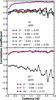 |
Fig. 4 Correlation coefficients for various pairs of ions obtained for period T2 plotted versus cadence. Additionally, the average correlation coefficient of all cadences with respective standard deviation are given. |
For both periods T1 and T2, the correlation coefficient between O+ and O6+, , is significantly larger than between O+ and solar-wind H+,  . This result indicates that the flux of inner-source pickup O+ is directly correlated with the flux of solar-wind O6+. We argue that this correlation can be interpreted as a direct correlation of inner-source and total solar-wind oxygen flux, for the following reasons. First, O6+ is the dominant charge state of oxygen in the solar wind and therefore already a good indicator of the total solar-wind oxygen flux. Second, the variability of the charge state distribution of oxygen depends on vsw (Zurbuchen et al. 1999). Using solar-wind speed-dependent expectation values,
  ), to determine the variability of O6+ assures that the variability of O6+ directly reflects the variability of solar-wind oxygen. Consequently, our results strongly imply that inner-source PUIs are produced by solar-wind neutralisation instead of solar-wind implantation.
Now we discuss whether the remaining correlation coefficients, , are also consistent with this scenario. From observations (von Steiger et al. 2000), it is known that the fraction of heavy ions in the solar wind is variable. Thus, the solar-wind elemental flux can be described as  (3)with solar-wind proton flux,
  and elemental fractionation, ηelm. In the neutralisation scenario, the production of neutrals is proportional to the solar-wind elemental flux and dust cross section. Inner-source pickup ions are born from these neutrals by ionisation, so that we get, for the elemental inner-source flux,
  (4)with elemental solar-wind flux,
  , dust cross section σdust, and total ionisation rate βelm. Total ionisation rates βelm are governed by photoionisation,
  , electron-impact ionisation,
  , and charge exhange with solar wind protons,
  ,
,  (5)The relative importance of the three consituents of βelm have been estimated for energetic neutral oxygen atoms by Bzowski et al. (2013). They find that charge exchange and photoionisation are equally important and that electron impact is negligible in the analysed period. Considering cross sections for charge exchange from Lindsay & Stebbings (2005) and low differential velocities vO–vsw, as expected from solar-wind neutralisation, charge exchange is much less important for inner-source neutral compared to energetic neutral oxygen. Consequently, we argue that βO is determined by
  . To our knowledge there are no comparable calculations for carbon, but in general charge exchange is expected to be even less important for carbon (Ruciński et al. 1996) owing to the quasi resonance of oxygen and protons. Comparing photionisation and electron impact ionisation cross sections for carbon and oxygen (NIST 2014), one finds that
  , and thus βC is also determined by
  . With
  for carbon and oxygen, we obtain from Eq. (4).
 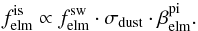 (6)Combining Eqs. (3) and (6), we get
 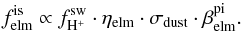 (7)Considering that
  is very similar to we argue due to Eq. (7) that the variability of the product,
  , is small compared to ηelm. Because measurements of the solar-wind carbon-to-oxygen ratio show only a small variability (von Steiger et al. 2000), i.e. ηC ≈ ηO, we expect that is very similar to , in accordance with our observations. In particular, our results are compatible with the idea that solar-wind carbon correlates with inner-source pickup C+. That the strongest correlation is found between C+ and O+ additionally supports this conclusion. Consider that ηC ≈ ηO and that σdust is the same for carbon and oxygen, it follows from Eq. (7) that C+/O+ would only vary like βC/βO. Thus, the strong correlation,
  , indicates only a minor variability of βC/βO.
The correlation coefficients for different cadences as shown in Fig. 4 clearly show that the correlations exist on all timescales, reaching from 2.5 h up to 3 days. A systematic decrease in sub-day cadences in all  and
and  could be explained by spatial diffusion of PUIs. Diffusion would inherently weaken the observed correlations. But we would like to point out that the observed decrease is most likely attributed to the low counting statistics of both ions, leading to a discretisation in the variability calculated according to Eq. (2). This interpretation is supported by the fact that this decrease is strongest in
  . Furthermore our results, i.e. the overall strong correlation coefficients, indicate that spatial diffusion is weak for inner-source PUIs.
Table 1 shows the correlation coefficients for two different time periods T1 and T2 as defined in Sect. 3.2. A comparison between T1 and T2 reveals a significant increase in and that is not visible for and  . The significant increase in and is attributed to the period from DoY 194.5 to 197.5, which is marked in red in Fig. 3 and which have been removed for T2. In this period, both O+ and C+ are equally enriched compared to O6+, are consistently very similar for T1 and T2. Consideration of Eq. (4) as either the dust cross section σdust, the ionisation rates , or both is significantly increased for this period. As mentioned in the previous section, this period might be influenced by a CME, although no signature of an ICME has been observed. On the other hand, measurements of the Solar Extreme ultraviolet Monitor, which is also part of CELIAS show only minor changes of ±5% in the UV flux for the analysed period. Thus, we do not expect a significant change in the ionisation rates. What can be seen, however, is a small spike that coincides with the expected CME injection time deduced from LASCO observations. Given that CMEs are expected to pick up nm-size dust grains Allegrini et al. (2005), it is possible that the dust cross section has been temporarily increased, if the outer boundaries of the CME have grazed SOHO. This dust pickup process has been discussed as the main argument against the neutralisation scenario Allegrini et al. (2005), because the resulting solar-cycle dependence of the inner source has not been observed. However, this finding is based on fewer than 200 counts of C+ and O+, respectively, while the increased fluxes observed by CTOF from DoY 194.5 to 197.5 are based on a total of 918 and 719 counts for C+ and O+, respectively. In addition, the study of the solar-cycle dependence was based on observations at ~70° heliographic latitude. Gopalswamy et al. (2003) found a north-south asymmetry of CMEs during that period of solar-maximum condition. In fact, in the nothern hemisphere where the Ulysses observations has been obtained, no CME above 60° has been observed. Thus, the conclusion that the inner source is stable over the solar cycle is not necessarily true on global scales.
5. Conclusions
Previous findings by Allegrini et al. (2005) have pointed towards a correlation of solar wind H+ flux with the count rates of inner-source O+ and C+. The C+ and O+ count rates obtained by Ulysses/SWICS at ~2 AU and roughly ± 70° heliographic latitude were increased for solar-wind H+ fluxes above 2 × 108 cm-2 s-1 compared to fluxes below this value. This has been interpreted as a hint towards a possible correlation of the solar-wind proton and inner-source PUI flux. In this study we have addressed this possible correlation using SOHO/CELIAS observations.
The unrivalled counting statistic of the CTOF instrument allowed us to show that the flux of inner-source O+ and C+ is highly variable. Daily fluxes show a strong variability roughly in the range ± 50% compared to the mean flux observed in the analysed period from DoY 150 to 220 in 1996. We calculated the variability for various cadences from ~2.5 h up to 3 days and found that O+ and C+ correlate with the flux of solar-wind O6+ with  ±0.02, and
  ±0.02, respectively. This correlation, which is significantly stronger than
  ±0.05 and
  , can be interpreted as a direct correlation of inner-source and solar-wind elemental flux. A decrease in the obtained correlation coefficients for sub-day cadences is most probably due to the low counting statistic of O+ and C+, but we cannot rule out the possibility that this decrease is partly real. A physical explanation for this decrease could be weak spatial diffusion of inner-source PUIs. However, even the highest cadence of ~2.5 h shows a strong correlation, and the overall strong correlation coefficients indicate that spatial dispersion of inner-source PUIs is globally weak.
Regarding the scenarios for the nature of the inner source for pickup ions, our results clearly point towards the solar-wind neutralisation scenario, because of its instantaneous production mechanism. Owing to the long delay between implantation in and re-emitting from dust grains, the solar-wind recycling scenario is not expected to show the observed correlation but rather the opposite result of a strong correlation with the solar-wind H+ flux. The found correlations among all analysed ions, H+, O6+, O+, and C+, agree with the expectations from solar-wind neutralisation. Especially the moderate correlation of O+ and H+, which has been indicated by previous findings, is not due to a direct causal relationship but rather a consequence of a moderate correlation of O6+ and H+. Although the main driver for the observed variability of inner-source oxygen is the variability of solar-wind oxygen with  , the even stronger correlation of inner-source carbon and oxygen with
  points towards a small variability of the dust cross section, the ionisation rates, or both.
In the analysed period from DoY 150 to 220, the continous interval from DoY 194.5 to 197.5 showed increased inner-source fluxes that might be related to a CME-related increase in the dust cross section. This possible CME-dust interaction, which has previously been the main argument against the solar-wind neutralisation scenario, requires further investigation. Especially the stability of the inner-source over the solar cycle, which has only been observed at high solar latitudes, should be investigated in the ecliptic.
In summary, our results clearly suggest that the solar wind is directly involved in the production of inner-source pickup ions, confirming and adding to previous studies that found a solar-wind-related composition of the inner source. Among the two proposed scenarios for the nature of the inner source that directly incorporate the solar wind, previous findings, and the findings presented in this study can be explained solely by the solar-wind neutralisation scenario.
Acknowledgments
This work was funded by DLR-Grant 50 OC 1103. Proton Monitor data has been provided by the SOHO archive. The LASCO CME catalogue is generated and maintained at the CDAW Data Center by NASA and The Catholic University of America in cooperation with the Naval Research Laboratory. SOHO is a project of international cooperation between ESA and NASA. Solar Extreme ultraviolet Monitor data has been taken from http://www.usc.edu/dept/space_science/instrument_pages/sem.htm.
References
- Allegrini, F., Schwadron, N. A., McComas, D. J., Gloeckler, G., & Geiss, J. 2005, J. Geophys. Res., 110, A05105 [Google Scholar]
- Berger, L., Drews, C., Taut, A., & Wimmer-Schweingruber, R. F. 2012, Proc. SW13 [Google Scholar]
- Bochsler, P., Möbius, E., & Wimmer-Schweingruber, R. F. 2006, Geophys. Res. Lett., 33, 6102 [NASA ADS] [CrossRef] [Google Scholar]
- Bochsler, P., Möbius, E., & Wimmer-Schweingruber, R. F. 2007, ESA SP, 641, 47 [NASA ADS] [Google Scholar]
- Bzowski, M., & Krolikowska, M. 2005, A&A, 435, 723 [NASA ADS] [CrossRef] [EDP Sciences] [Google Scholar]
- Bzowski, M., Sokół, J. M., Kubiak, M. A., & Kucharek, H. 2013, A&A, 557, A50 [NASA ADS] [CrossRef] [EDP Sciences] [Google Scholar]
- Cane, H. V., & Richardson, I. G. 2003, J. Geophys. Res., 108, 1156 [Google Scholar]
- Fahr, H. J. 1974, Space Sci. Res., 15, 483 [Google Scholar]
- Geiss, J., Gloeckler, G., Fisk, L. A., & von Steiger, R. 1995, J. Geophys. Res., 100, 23,373 [Google Scholar]
- Geiss, J., Gloeckler, G., & von Steiger, R. 1996, Space Sci. Rev., 78, 43 [NASA ADS] [CrossRef] [Google Scholar]
- Gloeckler, G., Fisk, L. A., Geiss, J., Schwadron, N. A., & Zurbuchen, T. H. 2000, J. Geophys. Res., 105, 7459 [NASA ADS] [CrossRef] [Google Scholar]
- Gopalswamy, N., Lara, A., Yashiro, S., & Howard, R. A. 2003, ApJ, 598, L63 [NASA ADS] [CrossRef] [Google Scholar]
- Grünwaldt, H., Neugebauer, M., Hilchenbach, M., et al. 1997, Geophys. Res. Lett., 24, 1163 [NASA ADS] [CrossRef] [Google Scholar]
- Hefti, S. 1997, Ph.D. Thesis, University of Bern [Google Scholar]
- Hovestadt, D., Hilechenbach, M., Bürgi, A., et al. 1995, Sol. Phys., 162, 441 [NASA ADS] [CrossRef] [Google Scholar]
- Lindsay, B. G., & Stebbings, R. F. 2005, J. Geophys. Res. Space Phys., 110, 12213 [NASA ADS] [CrossRef] [Google Scholar]
- Mann, I., & Czechowski, A. 2005, ApJ, 621, L73 [NASA ADS] [CrossRef] [Google Scholar]
- Moebius, E., Hovestadt, D., Klecker, B., Scholer, M., & Gloeckler, G. 1985, Nature, 318, 426 [NASA ADS] [CrossRef] [Google Scholar]
- National Institute of Standards and Technology 2014, http://www.nist.gov [Google Scholar]
- Ruciński, D., Cummings, A. C., Gloeckler, G., et al. 1996, Space Sci. Rev., 78, 73 [NASA ADS] [CrossRef] [Google Scholar]
- Schwadron, N. A., Geiss, J., Fisk, L. A., et al. 2000, J. Geophys. Res., 105, 7465 [NASA ADS] [CrossRef] [Google Scholar]
- Taut, A., Berger, L., Drews, C., & Wimmer-Scheingruber, R. F. 2015, A&A, 576, A55 [NASA ADS] [CrossRef] [EDP Sciences] [Google Scholar]
- von Steiger, R., Schwadron, N. A., Fisk, L. A., et al. 2000, J. Geophys. Res., 105, 27217 [NASA ADS] [CrossRef] [Google Scholar]
- Wimmer-Schweingruber, R. F., & Bochsler, P. 2003, Geophys. Res. Lett., 30, 1077 [NASA ADS] [CrossRef] [Google Scholar]
- Zurbuchen, T. H., Hefti, S., Fisk, L. A., Gloeckler, G., & von Steiger, R. 1999, Space Sci. Rev., 87, 353 [NASA ADS] [CrossRef] [Google Scholar]
All Tables
Mean correlation coefficients (ion2 = row, ion1 = column), and their standard deviations for the two periods T1 and T2 are given.
All Figures
|
Fig. 1 Time series of CTOF count rates for inner-source C+ and O+, and solar-wind O6+ (upper sub-panels) and PM solar-wind speed and flux vsw and fsw (lower sub-panels) are shown for daily, hourly, and 5-min cadences (top, middle, bottom panel). |
| In the text | |
|
Fig. 2 Illustration how O+ daily variabilities are derived. Top main
panel: 5-min solar-wind speeds vsw(t)
(top, left) and expectation values
|
| In the text | |
|
Fig. 3 Daily variabilities of various pairs of ions are plotted against each other. The colour indicates values that correspond to certain periods (see Sect. 3.2). |
| In the text | |
|
Fig. 4 Correlation coefficients for various pairs of ions obtained for period T2 plotted versus cadence. Additionally, the average correlation coefficient of all cadences with respective standard deviation are given. |
| In the text | |
Current usage metrics show cumulative count of Article Views (full-text article views including HTML views, PDF and ePub downloads, according to the available data) and Abstracts Views on Vision4Press platform.
Data correspond to usage on the plateform after 2015. The current usage metrics is available 48-96 hours after online publication and is updated daily on week days.
Initial download of the metrics may take a while.