| Issue |
A&A
Volume 576, April 2015
|
|
|---|---|---|
| Article Number | A53 | |
| Number of page(s) | 15 | |
| Section | Extragalactic astronomy | |
| DOI | https://doi.org/10.1051/0004-6361/201424913 | |
| Published online | 26 March 2015 | |
The ALHAMBRA survey: accurate merger fractions derived by PDF analysis of photometrically close pairs⋆,⋆⋆
1 Centro de Estudios de Física del Cosmos de Aragón, Plaza San Juan 1, 44001 Teruel, Spain
e-mail: This email address is being protected from spambots. You need JavaScript enabled to view it.
2 Instituto de Astrofísica de Andalucía (IAA-CSIC), Glorieta de la astronomía s/n, 18008 Granada, Spain
3 Institute for Computational Cosmology, Department of Physics, Durham University, South Road, Durham DH1 3LE, UK
4 GEPI, Observatoire de Paris, CNRS, Université Paris Diderot, 61 Avenue de l’Observatoire, 75014 Paris, France
5 Instituto de Física de Cantabria, Avenida de los Castros s/n, 39005 Santander, Spain
6 Observatori Astronòmic, Universitat de València, C/ Catedrático José Beltrán 2, 46980 Paterna, Spain
7 Observatório Nacional, COAA, Rua General José Cristino 77, 20921-400 Rio de Janeiro, Brazil
8 Instituto de Astrofísica de Canarias, vía Láctea s/n, La Laguna, 38200 Tenerife, Spain
9 Departamento de Astrofísica, Facultad de Física, Universidad de la Laguna, 38200 La Laguna, Spain
10 Department of Theoretical Physics, University of the Basque Country UPV/EHU, 48040 Bilbao, Spain
11 Departamento de Física Atómica, Molecular y Nuclear, Facultad de Física, Universidad de Sevilla, 41080 Sevilla, Spain
12 Institut de Ciències de l’Espai (IEEC-CSIC), Facultat de Ciéncies, Campus UAB, 08193 Bellaterra, Spain
13 Departamento de Astronomía, Pontificia Universidad Católica, Santiago, 782-0436 Macul, Chile
14 Departament d’Astronomia i Astrofísica, Universitat de València, 46100 Burjassot, Spain
Received: 3 September 2014
Accepted: 10 December 2014
Abstract
Aims. Our goal is to develop and test a novel methodology to compute accurate close-pair fractions with photometric redshifts.
Methods. We improved the currently used methodologies to estimate the merger fraction fm from photometric redshifts by (i) using the full probability distribution functions (PDFs) of the sources in redshift space; (ii) including the variation in the luminosity of the sources with z in both the sample selection and the luminosity ratio constrain; and (iii) splitting individual PDFs into red and blue spectral templates to reliably work with colour selections. We tested the performance of our new methodology with the PDFs provided by the ALHAMBRA photometric survey.
Results. The merger fractions and rates from the ALHAMBRA survey agree excellently well with those from spectroscopic work for both the general population and red and blue galaxies. With the merger rate of bright (MB ≤ −20−1.1z) galaxies evolving as (1 + z)n, the power-law index n is higher for blue galaxies (n = 2.7 ± 0.5) than for red galaxies (n = 1.3 ± 0.4), confirming previous results. Integrating the merger rate over cosmic time, we find that the average number of mergers per galaxy since z = 1 is Nmred = 0.57 ± 0.05 for red galaxies and Nmblue = 0.26 ± 0.02 for blue galaxies.
Conclusions. Our new methodology statistically exploits all the available information provided by photometric redshift codes and yields accurate measurements of the merger fraction by close pairs from using photometric redshifts alone. Current and future photometric surveys will benefit from this new methodology.
Key words: galaxies: evolution / galaxies: interactions / galaxies: statistics
Based on observations collected at the German-Spanish Astronomical Center, Calar Alto, jointly operated by the Max-Planck-Institut für Astronomie (MPIA) at Heidelberg and the Instituto de Astrofísica de Andalucía (CSIC).
The catalogues, probabilities, and figures of the ALHAMBRA close pairs detected in Sect. 5.1 are available at https://cloud.iaa.csic.es/alhambra/catalogues/ClosePairs
© ESO, 2015
1. Introduction
In their pioneering study, Toomre & Toomre (1972) were able to explain the tails and distortions of four peculiar galaxies as the intermediate stage of a merger event between two spiral galaxies. Since then, the role of mergers in galaxy evolution has been recognized and studied systematically, both observationally and theoretically. To constrain the role of mergers in galaxy evolution, two observational approaches are needed: understanding precisely how interactions modify the properties of galaxies and the fate of the merger remnants, and measuring the merger history of different populations over cosmic time to estimate the integrated effect of mergers.
Regarding the first approach, it is widely accepted today that the major merging (the merger of two galaxies with similar masses, M2/M1 ≥ 1/4) of two spiral galaxies is an efficient mechanism to create new bulge-dominated, red-sequence galaxies (Naab et al. 2006; Rothberg & Joseph 2006a,b; Hopkins et al. 2008; Rothberg & Fischer 2010; Bournaud et al. 2011), while major and minor mergers have been proposed as the main mechanism in the mass and size evolution of massive galaxies (e.g., Bezanson et al. 2009; López-Sanjuan et al. 2012). In addition, when the separation rp between galaxies in close pairs decreases, the star formation rate (SFR) is enhanced (Barton et al. 2000; Lambas et al. 2003; Robaina et al. 2009; Knapen & James 2009; Patton et al. 2011) and the metallicity decreases (Kewley et al. 2006; Ellison et al. 2008; Scudder et al. 2012).
Regarding the second approach, the merger history of a given population is estimated by measuring its merger fraction fm, that is, the fraction of galaxies in a sample that undergoes a merging process, both by morphological criteria (highly distorted galaxies are merger remnants, e.g., Conselice 2003; Conselice et al. 2008; Cassata et al. 2005; De Propris et al. 2007; Lotz et al. 2008, 2011; López-Sanjuan et al. 2009a,b; Jogee et al. 2009; Bridge et al. 2010), or by close-pair statistics (two galaxies close in the sky plane,  , and in redshift space, Δv ≤ 500 km s-1, that will lead to a merger, e.g., Le Fèvre et al. 2000; Patton et al. 2000, 2002; Patton & Atfield 2008; Lin et al. 2004, 2008; De Propris et al. 2005, 2010; de Ravel et al. 2009; de Ravel et al. 2011; López-Sanjuan et al. 2011, 2013; Tasca et al. 2014).
Several efforts have been conducted in the literature to study close companions in photometric surveys. Photometric surveys are limited by the Δv condition: The 500 km s-1 difference translates into a redshift difference of | z1 − z2| ≤ 0.0017(1 + z), with the best photometric redshifts (zp) from current broad+medium-band surveys reaching a precision ~0.01(1 + z) (e.g., Ilbert et al. 2009; Pérez-González et al. 2013; Molino et al. 2014). Next-generation large photometric redshift surveys will cover huge sky areas (≳5000 deg2) with broad-band filters, such as the Dark Energy Survey (DES, grizY; Flaugher 2012) and the Large Synoptic Survey Telescope (LSST, ugrizY; Ivezic et al. 2008), and with narrow-band filters, such as the Javalambre-Physics of the accelerated universe Astrophysical Survey (J-PAS, 56 optical filters of ~145 Å; Benítez et al. 2014), providing photometric redshifts for hundreds of million sources. Thus, a suitable and robust methodology to estimate the merger fraction from photometric close pairs is fundamental to exploit the current and the ambitious future photometric surveys.
The most extended approach to explore the redshift condition is estimating the number of random companions. It can be estimated by either searching for close companions in random positions in the sky, providing the number of expected companions found by chance in a given catalogue (e.g., Kartaltepe et al. 2007; Williams et al. 2011; Mármol-Queraltó et al. 2012; Xu et al. 2012; Díaz-García et al. 2013; Ruiz et al. 2014), or integrating the observed luminosity or mass function over the search area around the central galaxy (e.g., Le Fèvre et al. 2000; Rawat et al. 2008; Hsieh et al. 2008; Bluck et al. 2009; Bundy et al. 2009). Then, the observed number of companions is decontaminated by the random one to obtain the number of real companions.
A probabilistic approach was presented in López-Sanjuan et al. (2010, LS10 hereafter) to deal with the redshift condition. They assumed that the probability distribution function (PDF) of the photometric redshifts is well described by a Gaussian. Then, they estimated the overlap between the PDFs of close galaxies in the sky plane to derive the number of pairs per close system. In this approach, each system has a probability of being a real close pair.
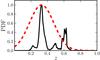 |
Fig. 1 Probability distribution function (PDF) of an ALHAMBRA source (black solid line) with I = 22.8 and its Gaussian approach (zp = 0.329 ± 0.147, red dashed line). Both distributions are normalised to their maximum probability. |
However, the previous methods have several shortcomings that should be addressed:
-
The PDFs of galaxies with a low signal-to-noise ra-tio are poorly approximated by a Gaussian func-tion. We illustrate this point in Fig. 1.The Gaussian approach of the PDF in this example iszp = 0.329 ± 0.147, notably worse than the actual PDF that presents two main narrow peaks at z ~ 0.33 and z ~ 0.61. Several studies have proven that the PDFs are the best approach to deal with photometric redshifts (e.g., Fernández-Soto et al. 2002; Cunha et al. 2009; Wittman 2009; Myers et al. 2009; Schmidt & Thorman 2013; Carrasco Kind & Brunner 2014).
-
The luminosity, stellar mass, or star formation rate of a source depend on its redshift. Even in the Gaussian approach, previous studies assumed the properties of galaxies to be constant with redshift, and they set them to the values of the best photometric redshift solution. This is a crude approximation that affects the sample selection as well as the luminosity and mass difference between galaxy pairs.
-
The colour selection is blurred by photometric errors. When blue galaxies spill over the red locus and vice versa, the differences between the two populations diminish for the galaxies with a low signal-to-noise ratio.
We here solve these shortcomings by generalising and extending the LS10 methodology. The new method (i) uses the full PDFs of the sources in redshift space; (ii) includes the variation in the luminosity of the sources with z in the sample selection and luminosity ratio constraint; and (iii) splits individual PDFs into red and blue spectral templates to reliable attend to the colour selections. We take advantage of the unique design, depth, and photometric redshift accuracy of the Advanced, Large, Homogeneous Area, Medium-Band Redshift Astronomical (ALHAMBRA1) photometric survey (Moles et al. 2008) to develop and test our new methodology.
ALHAMBRA survey fields.
The paper is organised as follows: in Sect. 2 we present the ALHAMBRA survey and its photometric redshifts. We develop the methodology to measure accurate merger fractions by PDF analysis of photometrically close pairs in Sect. 3. We test our new methodology by comparison with spectroscopic studies in Sects. 4 and 5, and in Sect. 6 we summarise our work and present our conclusions. Throughout this paper we use a standard cosmology with Ωm = 0.307, ΩΛ = 0.693, H0 = 100 h km s-1 Mpc-1, and h = 0.678 (Planck Collaboration XVI 2014). Magnitudes are given in the AB system (Oke & Gunn 1983).
2. ALHAMBRA survey
The ALHAMBRA survey provides a photometric data set over 20 contiguous, equal-width (~300 Å), non-overlapping, medium-band optical filters (3500–9700 Å) plus 3 standard broad-band near-infrared (NIR) filters (J, H, and Ks) over eight different regions of the northern sky (Moles et al. 2008). The survey has the aim of understanding the evolution of galaxies along cosmic time by sampling a large enough cosmological fraction of the Universe, for which reliable spectral energy distributions (SEDs) and precise photometric redshifts are needed. The simulations of Benítez et al. (2009), which relate the image depth and accuracy of the photometric redshifts to the number of filters, suggested that the filter set chosen for ALHAMBRA can achieve a photometric redshift precision that is three times better than a classical set of 4–5 optical broad-band filters. This expectation is confirmed by the results presented in Molino et al. (2014). The final survey parameters and scientific goals, as well as the technical properties of the filter set, were described by Moles et al. (2008). The survey has collected its data for the 20+3 optical-NIR filters with the 3.5 m telescope at the Calar Alto observatory, using the wide-field camera Large Area Imager for Calar Alto (LAICA) in the optical and the OMEGA–2000 camera in the NIR. The full characterisation, description, and performance of the ALHAMBRA optical photometric system were presented in Aparicio-Villegas et al. (2010). A summary of the optical reduction can be found in Cristóbal-Hornillos et al. (in prep.), the NIR reduction is reported in Cristóbal-Hornillos et al. (2009).
The ALHAMBRA survey has observed eight well-separated regions of the northern sky. The wide-field camera LAICA has four chips with a 15′ × 15′ field of view per chip (0.22 arcsec/pixel). The separation between chips is also 15′. Thus, each LAICA pointing provides four separated areas in the sky. Currently, six ALHAMBRA regions comprise two LAICA pointings. In these cases, the pointings define two separate strips in the sky. In our study, we assumed the four chips in each pointing to be independent sub-fields. The photometric calibration of the field ALHAMBRA-1 is currently ongoing, and the fields ALHAMBRA-4 and ALHAMBRA-5 comprise one pointing each (see Molino et al. 2014, for details). We summarise the properties of the seven ALHAMBRA fields used in Table 1. At the end, the data we used comprise 48 sub-fields of ~180 arcmin2 each, which can be assumed as independent for merger fraction studies as demonstrated by López-Sanjuan et al. (2014).
2.1. Bayesian photometric redshifts in ALHAMBRA
We relied on the ALHAMBRA photometric redshifts to compute the merger fraction. The photometric redshifts used throughout were fully presented and tested in Molino et al. (2014), and we summarise their principal characteristics below.
The photometric redshifts of ALHAMBRA were estimated with BPZ2.0, a new version of the Bayesian Photometric Redshift (BPZ; Benítez 2000) estimator. This is an SED-fitting method based on a Bayesian inference, where a maximum likelihood is weighted by a prior probability. The library of 11 SEDs that comprises four ellipticals (E), one lenticular (S0), two spirals (S), and four starbursts (SB), and the prior probabilities used by BPZ2.0 in ALHAMBRA are detailed in Benítez (in prep.). ALHAMBRA relied on the ColorPro software (Coe et al. 2006) to perform PSF-matched aperture-corrected photometry, which provided both total magnitudes and isophotal colours for the galaxies. In addition, an homogeneous photometric zero-point recalibration was made using either spectroscopic redshifts (when available) or accurate photometric redshifts from emission-line galaxies (Molino et al. 2014). Sources were detected in a synthetic F814W filter image, noted I in the following, defined to resemble the HST/F814W filter. The areas of the images affected by bright stars and those with lower exposure times (e.g., the edges of the images) were masked following Arnalte-Mur et al. (2014). The total area covered by the current ALHAMBRA data after masking is 2.38 deg2 (Table 1). Finally, a statistical star/galaxy separation is encoded in the variable Stellar_Flag of the ALHAMBRA catalogues, and we kept ALHAMBRA sources with Stellar˙Flag≤0.5 as galaxies.
The photometric redshift accuracy, as estimated by comparison with ~7200 spectroscopic redshifts (zs), is encoded in the normalised median absolute deviation (NMAD) of the photometric versus spectroscopic redshift distribution (Ilbert et al. 2006; Brammer et al. 2008), 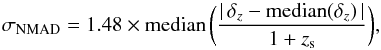 (1)where δz = zp − zs. The fraction of catastrophic outliers η is defined as the fraction of galaxies with | δz |/(1 + zs) > 0.2. In the case of ALHAMBRA, σNMAD = 0.011 for I ≤ 22.5 galaxies with a fraction of catastrophic outliers of η = 2.1%. We refer to Molino et al. (2014) for a more detailed discussion.
The odds quality parameter, noted  , is a proxy for the photometric redshift reliability of the sources and is also provided by BPZ2.0. The parameter is defined as the redshift probability enclosed on a ± K(1 + z) region around the main peak in the PDF of the source, where the constant K is specific for each photometric survey. Molino et al. (2014) found that K = 0.0125 is the optimal value for ALHAMBRA since this is the expected averaged accuracy for most galaxies in the survey. Thus,
 ![Mathematical equation: \hbox{$\mathcal{O} \in [0,1],$}](/articles/aa/full_html/2015/04/aa24913-14/aa24913-14-eq56.png) and it is related to the confidence of the photometric redshifts, making it possible to derive high-quality samples with better accuracy and a lower rate of catastrophic outliers. For example, an
and it is related to the confidence of the photometric redshifts, making it possible to derive high-quality samples with better accuracy and a lower rate of catastrophic outliers. For example, an  selection for I ≤ 22.5 galaxies yields σNMAD = 0.009 and η = 1%, while σNMAD = 0.006 and η = 0.8% if galaxies with
  are selected (see Molino et al. 2014, for further details). López-Sanjuan et al. (2014) set
  as the optimal selection for merger fraction studies in ALHAMBRA. We study the impact of this selection in Sect. 3.3.1.
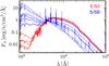 |
Fig. 2 Spectral energy distributions of the red (T = E/S0) and blue (T = S/SB) templates in BPZ2.0. The templates are normalised at λ = 4000 Å for clarity. (Colour version online.) |
2.2. Probability distribution functions in ALHAMBRA
This section is devoted to the description of the PDFs of the ALHAMBRA sources. The probability of a galaxy i to be located at redshift z and have a spectral type T is PDFi (z,T). This probability function is the posterior provided by BPZ2.0. The probability of the galaxy i to be located at redshift z is then (Fig. 1) 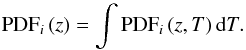 (2)Moreover, the total probability of the galaxy i of being located at z1 ≤ z ≤ z2 is
  (3)The distribution function PDF (z,T) is normalised to one by definition, meaning that there is one galaxy spread over the redshift and template spaces. Formally,
  (4)The definition of red and blue galaxies takes advantage of the profuse information encoded in the PDFs. Instead of selecting galaxies according to their observed colour or their best spectral template, we split each PDF into “red” templates (T = E/S0), noted PDFred, and “blue” templates (T = S/SB), noted PDFblue (Fig. 2). Formally,
  (5)In practice, the red templates have T ∈ [1,5.5] and the blue templates have T ∈ (5.5,11] in the ALHAMBRA catalogues. This is a major step forward in the methodology, which is able to reliably work with colour segregations without any pre-selection of the sources (Fig. 3).
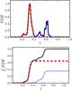 |
Fig. 3 Partial probability distribution functions (top panel) and the cumulative distribution functions (bottom panel) of the source presented in Fig. 1. The black solid lines mark the total PDF, the red dashed lines mark the red templates, PDFred = PDF (z,E/S0), and the blue dotted lines mark the blue templates, PDFblue = PDF (z,S/SB). This galaxy counts as 0.65 red and 0.35 blue in the analysis (bottom panel). |
The B-band absolute magnitude of a galaxy with observed magnitude I = 20 and spectral type T that is located at redshift z is noted as  , which is also provided by BPZ2.0. We are interested in MB as a function of z. We estimate MB (z) as
 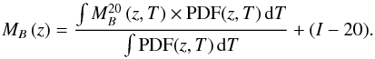 (6)The average B-band absolute magnitude of a galaxy is then
 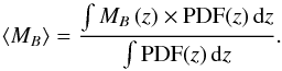 (7)Thanks to the probability functions defined in this section, we are able to statistically use the output of current photometric redshift codes without losing information. This is important to perform accurate and robust studies of the merger fraction and the environment with photometric redshifts.
2.3. Sample selection
Throughout this paper, we focus our analysis on the galaxies in the ALHAMBRA first data release2. This catalogue comprises ~500 k sources and is complete (5σ, 3″ aperture) for I ≤ 24.5 galaxies (Molino et al. 2014).
We performed our study in a given redshift range z ∈ [zmin,zmax) and in samples selected with B-band luminosity. To define the galaxy samples under study, we first estimated the B-band selection function,  , as
, as 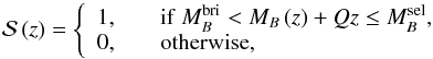 (8)where MB(z) is the B-band luminosity of the galaxy from Eq. (6), the term Qz accounts for the evolution of the luminosity function with redshift (e.g., Lin et al. 2008),
  is the selection magnitude of the sample, and
  imposes a maximum luminosity in the study. We assumed
  to avoid the different clustering properties of the brightest galaxies (Patton et al. 2000, 2002; Lin et al. 2008). Then, we kept as galaxies in the sample the sources with
 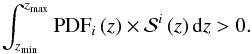 (9)The samples we studied comprise galaxies brighter than MB = −19 at the redshift ranges of interest. Given the depth of the ALHAMBRA data, these samples are volume-limited, and therefore no completeness correction is needed.
We note that Eq. (8) defines a B-band luminosity selection, but the selection function can be defined in the same way for mass-selected samples if the stellar mass M⋆ (z) of the sources is known.
3. Measuring the merger fraction in photometric samples by PDF analysis
In this section, we first recall the methodology to compute the merger fraction from spectroscopically close pairs (Sect. 3.1) and then extend the method to the photometric redshift regime (Sects. 3.2 and 3.4). The statistical weights devoted to correcting for the selection effects in the photometric case are defined in Sect. 3.3. Finally, the output of the code is detailed in Sect. 3.5.
3.1. Merger fraction in spectroscopic samples
The linear distance between two sources can be obtained from their projected separation, rp = θdA(z1), and their rest-frame relative velocity along the line of sight, Δv = c |z2 − z1|/(1 + z1), where z1 and z2 are the redshift of the central (the most luminous galaxy in the pair) and the satellite galaxy, respectively; θ is the angular separation, in arcsec, of the two galaxies on the sky plane; and dA(z) is the angular diameter distance, in kpc arcsec-1, at redshift z. Two galaxies are defined as a close pair if  and Δv ≤ Δvmax. To ensure clearly de-blended sources and to minimise colour contamination in ground-based surveys, the minimum search radius is usually
  kpc. With
  kpc and Δvmax ≤ 500 km s-1, 50% to 70% of the selected close pairs will finally merge (Patton et al. 2000; Patton & Atfield 2008; Bell et al. 2006; Jian et al. 2012).
To compute the merger fraction, one defines a primary and a secondary sample. The primary sample comprises the population of interest and one looks for those galaxies in the secondary sample that fulfil the close pair criterion for each galaxy of the primary sample. With the previous definitions, the merger fraction is  (10)where N1 is the number of sources in the primary sample and Np the number of close pairs. This definition applies to spectroscopic volume-limited samples, but we relied on photometric redshifts to compute fm. In the following, we expand the methodology presented by LS10 to use an arbitrary PDF in redshift space and to take into account the variation of galaxy properties with z.
3.2. PDF analysis of photometric close pairs
In this section, we detail the steps of computing the merger fraction in photometric redshift surveys. The primary and the secondary samples were defined according to the B-band selection function introduced in Sect. 2.3, noted  for the primary sample and
  for the secondary sample.
3.2.1. Initial list of projected companions
To define the initial list of projected close companions, we estimated the maximum angular separation possible in the first instance, noted θtop. This angular separation is defined as 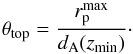 (11)Then, for each galaxy in the primary sample, we searched for galaxies in the secondary sample with θ ≤ θtop. We ended this first step with a list of systems composed of a principal source and its projected companions.
To illustrate the performance of our method and for the sake of clarity, we present a particular ALHAMBRA system as an example in the following. We defined the primary sample with absolute B-band magnitude  and the secondary sample with
  , and assumed an evolution in the selection of Q = 1.1. We used
  kpc as the smallest search radius,
  kpc as the largest search radius, zmin = 0.4 as the lowest redshift, and zmax = 1 as the highest redshift. These parameters are similar to those used in Sect. 5. The principal galaxy of the “system zero” is located at α1 = 188.7021 and δ1 = 61.9441. We found θtop = 13.32″ with the assumed parameters. We searched for companions in the secondary sample and found three projected companions (Fig. 4). We note that the companions a and b are also in the primary sample.
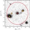 |
Fig. 4 Postage stamp of a particular ALHAMBRA system composed of a principal source (red cross) and its three projected companions in the sky plane (orange letters) in the I band. North is up and east to the left. The axes show the right ascension (α) and declination (δ) offset with respect to the position of the principal source (α1 = 188.7021, δ1 = 61.9441). The red circle marks the angular separation in the sky plane for |
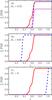 |
Fig. 5 Cumulative distribution function of the principal galaxy (red solid line), its projected companions (blue dashed lines), and the |
3.2.2. Redshift probability 
In the initial list defined above, a galaxy can have more than one projected companion. In that case, we took each possible pair separately, that is, if the companion galaxies a, b, and c are close to the principal galaxy X (Fig. 4), we studied the central-satellite pairs X–a, X–b, and X–c independently. This defines the initial list of projected close pairs. We note that if the galaxies X and a are both in the primary sample, the close pairs X–a and a–X could be present in the initial list. We cleaned the initial list from duplicates before starting the study in the redshift space, keeping the galaxy with lower ⟨ MB ⟩ as the central galaxy in the pair.
For each projected close pair in the initial list, we defined the redshift probability function as 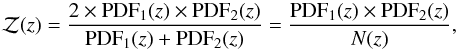 (12)where
 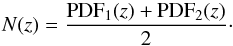 (13)We multiplied the PDFs of the central galaxy (PDF1) and its satellite (PDF2) to obtain the shape of the function , and we normalised by the number of potential pairs (two galaxies per pair) at each redshift, noted N(z). We note that ∫N(z) dz = 1 by construction. This normalisation is crucial in the methodology because it brings the close-pair systems to a common scale, with
  being the number of close pairs in the system at redshift z. Thus, the integral of the function provides the total number of pairs in the system,
  . We only kept projected close pairs with
  in the subsequent analysis.
We note that the velocity condition Δv ≤ 500 km s-1 used in spectroscopic studies (Sect. 4) is not included in the definition of the function . To account for the velocity condition, we should convolve the PDFs of the galaxies with a top-hat function. Formally,  (14)where W is a top-hat function of width 2Δvmax at redshift z. Then, we used the PDFΔv functions instead of the original PDFs in Eq. (12). The accuracy of the ALHAMBRA photometric redshifts is ~3000 km s-1, higher that the typical Δvmax condition. This implies that the ALHAMBRA PDFs are already smooth at the scale of the velocity condition, and a limited impact on the results is expected. We find that the convolution modifies the measured merger fractions by less than 1%, confirming our initial guess, but increases the computational time by a factor of 100. The convolution with a top-hat function can therefore be omitted in ALHAMBRA, but would be important for future medium-band photometric surveys, such as J-PAS, which will reach a precision of ~1000 km s-1.
The cumulative PDFs and the derived functions for the three projected close pairs in the “system zero” are shown in Fig. 5. The PDF of the central galaxy is the same in all the panels, with the best photometric redshift zp,1 = 0.604. The first companion, panel a, has a photometric redshift zp,2 = 0.630 and the overlap of the PDFs is evident, with  . The second companion, panel b, has zp,2 = 0.350 and the PDFs overlap marginally, with
  . Despite the low probability of this close pair, we kept it in the subsequent analysis because
  . The third companion, panel c, has zp,2 = 0.988 and the PDFs do not overlap, with
  . Thus, we discard this close pair in the following.
3.2.3. Angular mask ℳθ
 |
Fig. 6 Angular separation θ as a function of redshift. The solid lines mark the measured angular separation of the close pairs, θ = 7.36″ in panel a) and θ = 10.46″ in panel b). The letter in each panel refers to the companion galaxy in Fig. 4. The grey area marks the angular separations between θmin (z) and θmax (z) (red dashed lines). The vertical dashed lines mark the redshift range under study, 0.4 ≤ z< 1. The redshifts at which the angular mask ℳθ is equal to one are marked with the thick green line. |
The function defined in the previous section only accounts for the overlap of the central and the satellite galaxy probabilities in redshift space. However, the definition of a close pair also includes conditions on the projected distance rp and on the luminosity of the sources. Thus, the next step was to define redshift masks, noted ℳ (z), to account for the other conditions of interest. These masks complement the function and are equal to one at redshifts where a particular condition is fulfilled and equal to zero otherwise.
The first mask that we computed is the angular mask ℳθ. The function dA changes with redshift, which means that a close pair in the sky plane at zmin (Sect. 3.2.1) might not be a close pair at higher redshifts. Thus, we estimated the functions 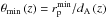 and
and 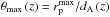 , and imposed the condition θmin (z) ≤ θ ≤ θmax (z). Formally,
 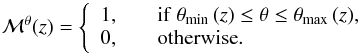 (15)The measured angular separation of the close pairs in the “system zero” are shown in Fig. 6. The first pair, panel a, has θ = 7.36″ and fulfils the angular condition at z> 0.106. The second pair, panel b, has θ = 10.46″ and fulfils the angular condition in two redshift ranges, 0.071 <z< 0.663 and z> 4.099 (outside the plotted redshift range). We focused here on z< 1, but the method has been developed to study close pairs in the full redshift space.
3.2.4. Pair selection mask ℳpair
In this section we define the pair selection mask, noted ℳpair(z). The pair selection mask simultaneously imposes three conditions: the selection of the primary sample, the selection of the companion sample, and the luminosity ratio between the galaxies in the pair. The last condition is needed to define major and minor companions. Formally, the general form of the pair selection mask is 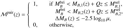 (16)where ΔMB (z) = |MB,2(z) − MB,1(z) | and μ = LB,2/LB,1 is the B-band luminosity ratio. Typically, μ ≥ 1/4 (ΔMB ≤ 1.5) defines major mergers, and μ< 1/4 defines minor mergers (e.g., López-Sanjuan et al. 2011). We recall that we assumed (Sect. 2.3). We note that Eq. (16) focuses on a B-band luminosity selection, but the pair selection mask can be defined in the same way for mass-selected pairs if the stellar mass M⋆(z) of the sources is known.
The MB (z) function of the principal galaxy and its companions in the “system zero” are shown in Fig. 7, the derived luminosity ratios in Fig. 8. We assumed μ = 1/4 to select major companions. The first companion, panel a in both figures, is fainter than the central galaxy at each redshift with ΔMB ~ 0.6. This value is higher than the luminosity difference derived from the best-fit solution, ΔMB = 0.47. We note that the principal galaxy fulfils the primary selection at z> 0.52. The second companion, panel b in both figures, is brighter than the principal galaxy at each redshift with ΔMB ≥ 1.2, far from the best-fit solution ratio, ΔMB = 0.22. The principal galaxy has a lower ⟨ MB ⟩ than the companion and was assumed to be the central galaxy of the pair (Sect. 3.2.2). However, the study of MB (z) reveals that the companion is indeed the central galaxy, and the principal galaxy of the “system zero” its satellite. In consequence, the companion has to fulfil the primary selection and the principal galaxy the secondary selection in Eq. (16). This case illustrates the possible complexity of the systems under study and the importance of analysing the physical variables in the redshift space.
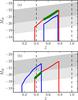 |
Fig. 7 B-band absolute magnitude MB as a function of redshift. The red and blue solid lines mark the absolute magnitude of the principal and the companion galaxy, respectively, at redshifts with PDF (z) > 0. The letter in each panel refers to the companion galaxy in Fig. 4. The dark grey area marks the selection of the primary sample, and the two grey areas mark the selection of the secondary sample (i.e., the primary sample is included in the secondary one). The vertical dashed lines mark the redshift range under study, 0.4 ≤ z< 1. The redshifts at which the pair selection mask ℳpair is equal to one are marked with the thick green line. (Colour version online.) |
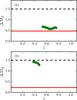 |
Fig. 8 Absolute magnitude difference between the galaxies in the pair, ΔMB (z) = |MB,2(z) − MB,1(z) |, as a function of redshift (thick green line). The letter in each panel refers to the companion galaxy in Fig. 4. The dashed lines mark the major merger limit, ΔMB = 1.5. The red solid lines mark the ΔMB computed with the absolute magnitudes estimated at the best photometric redshifts. |
3.2.5. Pair probability function
Finally, each close-pair system has an associated pair probability function defined as  (17)where is the redshift probability function (Sect. 3.2.2), ℳθ is the angular mask (Sect. 3.2.3), and ℳpair is the pair selection mask (Sect. 3.2.3) of the system. The PPF is a new probability function3 that encodes the relevant information about the close pairs in the survey. The PPFs are used to define the number of pairs (Sect. 3.4), but are also crucial for subsequent studies of properties of galaxies with a close companion, such as the star formation rate. We will explore the potential of the PPFs in a future work.
3.3. Correction for selection effects
The PPFs defined in the previous section are mainly affected by two selection effects in ALHAMBRA: the selection in the odds parameter (Sect. 3.3.1) and the incompleteness in the search volume near the image boundaries (Sect. 3.3.2). In the next sections, we define the statistical weights devoted to correcting for these selection effects.
3.3.1. odds sampling rate
Following spectroscopic studies, we should correct the raw PPFs for the selection effects in our sample. As shown by Molino et al. (2014), a selection in the parameter ensures high-quality photometric redshifts and a low rate of catastrophic outliers. López-Sanjuan et al. (2014) set as the optimal selection for merger fraction studies in ALHAMBRA. If the galaxies with  are included in the samples, the projection effects become strong and the merger fraction is overestimated.
We defined the odds sampling rate (OSR) as the ratio of galaxies with with respect to the total number of galaxies (i.e., those with  ). The OSR mainly depends on the I-band magnitude because the quality of the photometric redshifts decreases according to the signal-to-noise ratio. We used the redshift information encoded in the PDFs to estimate the OSR in our range of interest. Formally, the odds sampling rate of the ALHAMBRA sub-field j is estimated as
 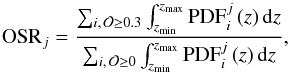 (18)where i indexes every galaxy in the sub-field j.
The current ALHAMBRA release comprises 48 sub-fields. To estimate the global OSR in ALHAMBRA, we computed  (19)where
  is the inverse of the number density in the sub-field j. This density weight avoids the global OSR to be dominated by the densest ALHAMBRA sub-fields.
We computed the OSRALH in bins of 0.5 magnitudes in the I band at 0.4 ≤ z< 1 and interpolated the results to obtain OSRALH (I). We checked that our interpolated function describes the OSRALH properly estimating it in bins of 0.1 magnitudes (Fig. 9). Finally, we defined the odds weight of the galaxy i as 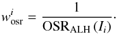 (20)The odds weight only depends on the I-band magnitude of the galaxy, and we checked that it slightly depends on redshift in our range of interest.
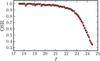 |
Fig. 9 Odds sampling rate (OSR) in ALHAMBRA as a function of the I-band magnitude. Dots are the OSR estimated at 0.4 ≤ z< 1 in bins of 0.1 magnitudes. The solid line is the functional parametrisation of the OSR used in the paper. |
3.3.2. Border effects in the sky plane
When we search for a primary source companion, we define a volume in the sky plane-redshift space. If the primary source is near the boundaries of the survey, a fraction of the search volume lies outside of the effective volume of the survey. We defined the area weight of a close pair system as 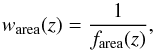 (21)where farea is the fraction of the search area that is covered by the ALHAMBRA survey. The search area is a ring centred at (α1,δ1) and defined by
  and
and  . The search area, and therefore the area weight, depends on redshift because of the variation of the angular diameter distance dA with z.
3.3.3. Pair weight wpair
For each observed close pair we defined the pair weight as  (22)where wosr,1 = wosr (I1) is the odds weight of the central galaxy, wosr,2 = wosr (I2) is the odds weight of the satellite galaxy, and warea is the area weight of the pair. The pair weight is always equal to or larger than unity and is applied to volume-limited samples.
3.4. Merger fraction in photometric samples by PDF analysis
The merger fraction in the redshift range zr = [zmin,zmax) is 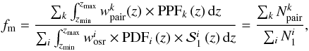 (23)where k indexes the close pair systems, i indexes the galaxies in the primary sample, PPF is the pair probability function (Sect. 3.2.5), wpair is the pair weight (Sect. 3.3.3), wosr is the odds weight of the primary galaxies (Sect. 3.3.1), and
  is the selection function of the primary galaxies (Sect. 2.3). Equation (23) is the photometric analogue of Eq. (10), with
  being the number of close pairs and
  the number of primary galaxies. To estimate the observational error of fm, noted σf, we used the jackknife technique (Efron 1982). We computed partial standard deviations for each system k, δk, taking the difference between the measured fm and the same quantity after removing the kth pair from the sample,
  , such that
  . For a redshift range with Np systems, the variance is given by
 ![Mathematical equation: \hbox{$\sigma_{f}^2 = [(N_{\rm p}-1) \sum_k \delta_k^2]/N_{\rm p}$}](/articles/aa/full_html/2015/04/aa24913-14/aa24913-14-eq228.png) .
.
ALHAMBRA close-pair catalogue.
3.5. Output of the code
In addition to the merger fraction, the developed code also provides valuable outputs for future studies. The code creates three files:
-
The close pair catalogue. It summarises the main properties of thepairs, as shown in Table 2. The reported values areeither integrated over zmin and zmax or the values for the best photometricredshift. However, we encourage the use of the PDFs and the PPFsas outlined throughout the paper.
-
The close pair probabilities. The relevant merger probabilities of the systems listed in the close-pair catalogue are stored in a hdf5 file. We report the PPF and the wpair of each close pair. The computation and the storage of the PPFs were made with PyTables4 (Alted et al. 2002).
-
A complete graphical output with the summary of each close pair with Npair ≥ 0.01. This summary includes the stamp of the merger system in the synthetic I band, the relevant information from the close-pair catalogue, the PDFs of the principal and companion galaxies, the function
, and the angular and the pair selection masks. We present an example of the graphical output of the code in Fig. 10.
Merger fraction in ALHAMBRA as a function of B band luminosity.
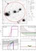 |
Fig. 10 Example of the graphical output of the code. Top panel: postage stamp of the close pair in the I band. The red cross marks the principal galaxy, the blue cross the companion galaxy. The red circle marks |
4. Merger fraction in ALHAMBRA
4.1. Reliable measurement of the merger fraction in ALHAMBRA
As demonstrated by López-Sanjuan et al. (2014), the 48 ALHAMBRA sub-fields can be assumed to be independent for merger fraction studies. In addition, they set the optimal parameters to obtain reliable merger fractions. The ALHAMBRA merger fractions we report here were computed as follows:
-
1.
The primary and secondary samples comprise galaxies with
.This ensures high-quality photometric redshifts and non-biasedsamples, as shown by López-Sanjuanet al. (2014). -
2.
The methodology presented in Sect. 3 was applied in each ALHAMBRA sub-field to obtain the merger fraction fm. This provided 48 estimations of fm across the sky.
-
3.
We applied the maximum likelihood estimator (MLE) presented in López-Sanjuan et al. (2014) to measure the average merger fraction in ALHAMBRA and its uncertainty. The MLE uses the measured merger fractions and their errors to compute the median of the merger fraction distribution. It also provides a reliable measurement of the intrinsic dispersion of the distribution, which is the cosmic variance. The cosmic variance for close-pair studies was studied in detail by López-Sanjuan et al. (2014). We stress that the reported ALHAMBRA merger fractions are unaffected by cosmic variance.
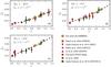 |
Fig. 11 Merger fraction fm as a function of redshift and selection in B band luminosity, panel a) for MB ≤ − 20 galaxies, panel b) for MB ≤ − 19.5 galaxies, and panel c) for MB ≤ − 19 galaxies. The orange stars are from the ALHAMBRA photometric survey (this work), the green squares from spectro-photometric pairs in GOODS-S (LS10), and the red symbols are from spectroscopic surveys: Hexagons from the SSRS2 (Patton et al. 2000), inverted triangles form the MGC (LS10), diamonds from the CNOC2 (Patton et al. 2002), dots from the VVDS-Deep (this work), triangles from the DEEP2 (Lin et al. 2004), and pentagons from Lin et al. (2008). The dashed lines are the best fit of Eq. (25) to the data. The power-law index from the best fit is labelled in the panels. |
4.2. Merger fraction in MB selected samples
We test the reliability of our new methodology by comparing the merger fractions in the ALHAMBRA photometric survey with those from previous spectroscopic work. Robust measurements in the B band from spectroscopic samples are available from the local Universe to z ~ 1, providing a valuable benchmark for our purposes. We used the homogenised compilation from LS10 to test the performance of the ALHAMBRA merger fractions. This compilation comprises the merger fractions from Patton et al. (2000) in the Second Southern Sky Redshift (SSRS2; da Costa et al. 1998) survey, LS10 in the Millennium Galaxy Catalogue (MGC; Liske et al. 2003; see also De Propris et al. 2005, 2007) and Great Observatories Origin Deep Survey South (GOODS-S; Giavalisco et al. 2004), Patton et al. (2002) in the Canadian Network for Observational Cosmology (CNOC2; Yee et al. 2000) survey, Lin et al. (2004) in the DEEP2 redshift survey (Newman et al. 2013), and Lin et al. (2008) in several of the above spectroscopic redshift surveys.
Following LS10, we defined three samples selected in B-band luminosity. These samples are defined with  , and −19, and no evolution in the selection, Q = 0. We used these three samples as primary and secondary samples (i.e.,
  ), and did not apply any luminosity condition between the galaxies in the pairs (μ = 0). We searched for close pairs with 6 h-1 kpc ≤ rp ≤ 21 h-1 kpc to mimic the definition used by LS10. We performed the study at 0.4 ≤ z< 1 to ensure large enough volumes at the lower redshifts and volume-limited samples at the higher ones. We summarise the ALHAMBRA merger fractions in Table 3 and show them in Fig. 11. We find that the merger fraction increases with redshift and that it is larger for fainter samples.
LS10 reported the number of companions Nc, which is twice the number of close pairs (two galaxies per pair). We show 0.5Nc therefore in Fig. 11. In addition, we computed the merger fraction in the deep part of the VIMOS VLT Deep Survey (VVDS; Le Fèvre et al. 2005, 2013) following Sect. 3.1 and the completeness corrections outlined in de Ravel et al. (2009) and López-Sanjuan et al. (2011). The ALHAMBRA merger fractions agree excellently well with the spectroscopic values. These results demonstrate that we can measure reliable and accurate merger fractions using photometric information alone.
4.3. Redshift evolution of the merger fraction in MB selected samples
We parametrised the redshift evolution of the merger fraction with a power-law (e.g., Le Fèvre et al. 2000), 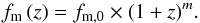 (24)Hereafter, the fittings were performed with emcee (Foreman-Mackey et al. 2013), a Python implementation of the affine-invariant ensemble sampler for Markov chain Monte Carlo (MCMC) proposed by Goodman & Weare (2010). emcee provides a collection of solutions in the parameter space, with the density of solutions being proportional to the posterior probability of the parameters. We obtained the best-fit values and their uncertainties as the median and the dispersion of the projected solutions. In addition, the correlation between the parameters, noted ρxy, is easily accessible.
We summarise the best fits to the data from Fig. 11 in Table 4. The power-law index m increases with the luminosity selection, with the merger fraction at z = 0 decreasing. In addition, the parameters show a clear anti-correlation, with ρxy ~ − 0.96 (Table 4). To illustrate this correlation, we show the probability contours of the fitted parameters in Fig. 12. The probability contours of the populations are different at more than 3σ, even if the inferred m values are compatible at the 2σ level. Thus, the observed trends are robust to the anti-correlation between fm,0 and m.
We estimated the dependence of fm,0 and m on the B-band luminosity selection by fitting the function ![Mathematical equation: \begin{equation} f_{\rm m}\,(z,M_B) = [f_{0} + \alpha(M_B + 20)]\times(1+z)^{m_0 + \beta(M_B + 20)}\label{ffzmb} \end{equation}](/articles/aa/full_html/2015/04/aa24913-14/aa24913-14-eq273.png) (25)to all the available data. We obtain f0 = 0.43 ± 0.05 %, α = 0.63 ± 0.09 %, m0 = 2.37 ± 0.17, and β = −0.62 ± 0.20. This global fitting is compatible with the individual parameters in Table 4 and implies that fm,0 = 2.84 − m% (Fig. 12). The observed trends were previously reported by Lin et al. (2004) and LS10, and they pointed out the importance of the selection when different merger fraction studies are compared.
(25)to all the available data. We obtain f0 = 0.43 ± 0.05 %, α = 0.63 ± 0.09 %, m0 = 2.37 ± 0.17, and β = −0.62 ± 0.20. This global fitting is compatible with the individual parameters in Table 4 and implies that fm,0 = 2.84 − m% (Fig. 12). The observed trends were previously reported by Lin et al. (2004) and LS10, and they pointed out the importance of the selection when different merger fraction studies are compared.
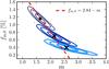 |
Fig. 12 Probability contours in the fm,0 vs. m plane as a function of the B-band luminosity selection (Table 4). The contours enclose 68.2%, 95.4% and 99.7% of the probability. The crosses mark the most probable values of the parameters, with the larger cross for the more luminous galaxies. The dashed line is from the Eq. (25) fit to the data, fm,0 = 2.84 − m. (Colour version online.) |
Redshift evolution of the merger fraction as a function of B-band luminosity.
5. Major merger rate in ALHAMBRA
The final goal of merger studies is estimating the merger rate Rm, defined as the number of mergers per galaxy and Gyr-1. The merger rate is computed from the merger fraction by close pairs as  (26)where the factor
  takes into account the lost companions at
  (Bell et al. 2006), and Cm is the fraction of the observed close pairs that finally merge after a merger time scale Tm. The merger time scale and the merger probability Cm should be estimated from simulations (e.g., Kitzbichler & White 2008; Lotz et al. 2010a,b; Lin et al. 2010; Jian et al. 2012; Moreno et al. 2013). On the one hand, Tm mainly depends on the search radius , the stellar mass of the central galaxy, and the mass ratio between the galaxies in the pair with a mild dependence on redshift and environment (Kitzbichler & White 2008; Jian et al. 2012). On the other hand, Cm mainly depends on and environment with a mild dependence on redshift and the mass ratio between the galaxies in the pair (Jian et al. 2012). Despite the efforts in the literature to estimate both Tm and Cm, different cosmological and galaxy formation models provide different values within a factor of two to three (e.g., Hopkins et al. 2010).
Major merger rate of MB ≤ − 20 − 1.1z galaxies in ALHAMBRA.
We used the merger time scales from Kitzbichler & White (2008) to translate our merger fractions and the merger fractions from the literature to a common scale. The Tm from Kitzbichler & White (2008) already includes the merger probability, so we assume Cm = 1 in the following.
5.1. Major merger rate of bright galaxies
In this section, we estimate the major merger rate RMM of bright galaxies in the ALHAMBRA survey and compare it with data from the literature. We defined primary galaxies with , taking Q = 1.1 as the evolution of the luminosity function with z (e.g., Ilbert et al. 2006). This selects galaxies brighter than  up to z = 1. We searched major companions with ΔMB ≤ 1.5 magnitudes (μ ≥ 1/4). The companion sample therefore comprises galaxies with and Q = 1.1.
We estimated the major merger rate from the merger fraction of 10 h-1 kpc ≤ rp ≤ 50 h-1 kpc close pairs, and following López-Sanjuan et al. (2011), we used Tm = 2.3 ± 0.3 Gyr. We summarise the ALHAMBRA merger rates in Table 5 and in Fig. 13. The major merger rate increases with redshift, in agreement with previous work (e.g., de Ravel et al. 2009). We tested the robustness of the ALHAMBRA results by comparing them with those from the VVDS-Deep and MGC spectroscopic surveys (López-Sanjuan et al. 2011). The ALHAMBRA data agree with the major merger rates from the VVDS-Deep at 0.3 <z< 1. We parametrised the major merger rate as  (27)The best fit to the ALHAMBRA, VVDS-Deep, and MGC data is presented in Table 6. We find RMM,0 = 0.029 ± 0.006 Gyr-1 and n = 1.7 ± 0.4. These values from the combined data set are consistent with those obtained from the ALHAMBRA data alone, with RMM,0 = 0.032 ± 0.013 Gyr-1 and n = 1.6 ± 0.7. These results further support our new methodology and the quality of the ALHAMBRA survey data.
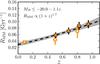 |
Fig. 13 Major merger rate RMM as a function of redshift for MB ≤ − 20 − 1.1z galaxies. The stars are from the ALHAMBRA photometric survey, the circles from the VVDS-Deep spectroscopic survey, and the inverted triangle from the MGC spectroscopic survey. The dashed line is the best fit of a power-law to the data. The power-law index of the best fit is labelled in the panel. The grey area marks the 68% confidence interval of the fit. |
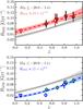 |
Fig. 14 Major merger rate RMM as a function of redshift and colour for MB ≤ −20−1.1z galaxies. The stars are from the ALHAMBRA photometric survey, the circles from the VVDS-Deep spectroscopic survey, and the inverted triangles from the MGC spectroscopic survey. The dashed line in both panels is the best fit of a power-law to the data. The power-law index of the best fit is labelled in the panels. The coloured area marks the 68% confidence interval of the fit. The dotted lines and the grey areas mark the best fit to the global population shown in Fig. 13. Top panel: red population, selected as galaxies with E/S0 templates in ALHAMBRA, galaxies with NUV − r ≥ 4.25 in the VVDS-Deep, and galaxies with u − r ≥ 2.1 in the MGC. Bottom panel: blue population, selected as galaxies with S/SB templates in ALHAMBRA, galaxies with NUV − r < 4.25 in the VVDS-Deep, and galaxies with u − r < 2.1 in the MGC. |
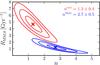 |
Fig. 15 Probability contours in the RMM,0 vs. n plane for red and blue galaxies. The contours enclose 68.2%, 95.4% and 99.7% of the probability. The crosses mark the most probable values of the parameters. The best power-law indices n are labelled in the panel. (Colour version online.) |
5.2. Major merger rate of red and blue galaxies
In this section we study the major merger rate of red (E/S0 templates) and blue (S/SB templates) galaxies. The primary and the secondary samples are defined as in the previous section. We estimated the major merger rate of red galaxies using the PDFred and of blue galaxies using the PDFblue. As noted in Sect. 2.2, we did not perform any colour selection of the sources, and all the galaxies in the primary sample were included in the analysis. This is a novel approach that is only possible thanks to the rich information encoded in the PDFs provided by BPZ2.0. We used the full PDFs of the companions, that is, we searched for all the possible companions of red and blue primary galaxies. Following López-Sanjuan et al. (2011), we used  Gyr for red galaxies and
  Gyr for blue galaxies (i.e., the blue galaxies are less massive than the red galaxies of similar B-band luminosity).
Major merger rate evolution of MB ≤ − 20 − 1.1z galaxies.
We summarise our results in Table 5 and Fig. 14. The major merger rate of red galaxies is higher than the major merger rate of blue galaxies at any redshift. As in the previous section, we compared the ALHAMBRA results with those from the VVDS-Deep and the MGC. López-Sanjuan et al. (2011) defined red galaxies in the VVDS-Deep with NUV − r ≥ 4.25 and blue galaxies with NUV − r< 4.25. In addition, we computed the red and blue merger rates in the MGC. We defined red galaxies with u − r ≥ 2.1 and blue galaxies with u − r< 2.1 (e.g., Strateva et al. 2001) thanks to the Sloan Digital Sky Survey (SDSS; Aihara et al. 2011) photometry. We find  Gyr-1 and
  Gyr-1 at z = 0.09. The ALHAMBRA major merger rates agree with the spectroscopic values.
We fit a power-law to the data and found that (Table 6)
-
the evolution of the red merger rate is
 (28)
(28) -
the evolution of the blue merger rate is
 (29)
(29) -
the blue merger rate evolves faster than the red merger rate, in agreement with previous results (e.g., Lin et al. 2008; de Ravel et al. 2009; Chou et al. 2011; López-Sanjuan et al. 2012; Lackner et al. 2014).
We note that the parameters in the fittings are anti-correlated (Table 5) and show the probability contours of the fitted parameters in the Fig. 15. This figure demonstrates that the fittings to the red and blue populations are different at more than 3σ, even if the indices n are compatible at the 2σ level. This anti-correlation also has an impact on the integrated merger history of red and blue galaxies, which is much better constrained than the individual parameters from the fitting. Integrating the merger rate over cosmic time, we find that the average number of mergers per galaxy since z = 1 is  for red galaxies and
  for blue galaxies. Thus, red galaxies have undergone about twice as many major mergers as blue galaxies since z = 1.
These results demonstrate that our new methodology naturally takes care of colour segregations and that accurate merger rates of red and blue galaxies can be estimated with photometric data alone.
6. Summary and conclusions
We have developed a new methodology to compute accurate merger fractions from a PDF analysis of photometrically close pairs. Our method solves the main shortcomings of previous merger fraction studies in photometric samples by (i) using the full PDF of the sources in redshift space; (ii) including the variation in the luminosity of individual sources with z in both the selection of the samples and in the luminosity ratio constrain; and (iii) splitting individual PDFs into red and blue spectral templates to reliably work with rest-frame colour selections.
We find that our methodology provides merger fractions and rates that nicely agree with those from spectroscopic work, both for the general population and for red and blue galaxies. With the merger rate of bright (MB ≤ − 20 − 1.1z) galaxies evolving as (1 + z)n, the power-law index n is higher for blue galaxies (n = 2.7 ± 0.5) than for red galaxies (n = 1.3 ± 0.4), confirming previous results. Integrating the merger rate over cosmic time, we find that the average number of mergers per galaxy since z = 1 is for red galaxies and for blue galaxies. Thus, red galaxies have undergone about twice as many major mergers as blue galaxies since z = 1.
We conclude that our new methodology provides accurate merger fractions from photometric data alone and reliably works with the available information in redshift and template spaces. We have tested the performance of our new methodology with the PDFs provided by the ALHAMBRA survey, but it can be applied to any current and future photometric survey, such as DES, J-PAS, or LSST.
In future work we will study the dependence of the merger fraction on the stellar mass or the morphology (see Pović et al. 2013 for details about the morphological classification in ALHAMBRA). In addition, the study of galaxy properties in paired galaxies will be performed thanks to the PPFs defined in the present work. Finally, the comparison of the observed trends with the expectations from cosmological models should be explored to better understand the role of mergers in galaxy evolution.
Formally, the PPF is not a probability density function because its normalisation is different from one. However, the integral of the PPF is a probability. Therefore we keep the attribute probability in the following.
Acknowledgments
We dedicate this paper to the memory of our six IAC colleagues and friends who met with a fatal accident in Piedra de los Cochinos, Tenerife, in February 2007, with special thanks to Maurizio Panniello, whose teachings of python were so important for this paper. We acknowledge the comments and suggestions of the anonymous referee. This work has been mainly funded by the FITE (Fondos de Inversiones de Teruel) and the projects AYA2012-30789, AYA2006-14056, and CSD2007-00060. We also acknowledge financial support from the Spanish Government grants AYA2010-15169, AYA2010-22111-C03-01, AYA2010-22111-C03-02, and AYA2013-48623-C2-2, from the Aragón Government through the Research Group E103, from the Junta de Andalucía through TIC-114 and the Excellence Project P08-TIC-03531, and from the Generalitat Valenciana through the projects Prometeo/2009/064 and PrometeoII/2014/060. A.J.C. is Ramón y Cajal fellow of the Spanish government. M.P. acknowledges the financial support from JAE-Doc program of the Spanish National Research Council (CSIC), co-funded by the European Social Fund. This research made use of Astropy, a community-developed core Python package for Astronomy (Astropy Collaboration et al. 2013), and Matplotlib, a 2D graphics package used for Python for publication-quality image generation across user interfaces and operating systems (Hunter 2007).
References
- Aihara, H., Allen de Prieto, C., An, D., et al. 2011, ApJS, 193, 29 [NASA ADS] [CrossRef] [Google Scholar]
- Alted, F., Vilata, I., Prater, S., et al. 2002, PyTables: Hierarchical Datasets in Python [Google Scholar]
- Aparicio-Villegas, T., Alfaro, E. J., Cabrera-Caño, J., et al. 2010, AJ, 139, 1242 [NASA ADS] [CrossRef] [Google Scholar]
- Arnalte-Mur, P., Martínez, V. J., Norberg, P., et al. 2014, MNRAS, 441, 1783 [NASA ADS] [CrossRef] [Google Scholar]
- Astropy Collaboration, Robitaille, T. P., Tollerud, E. J., et al. 2013, A&A, 558, A33 [NASA ADS] [CrossRef] [EDP Sciences] [Google Scholar]
- Barton, E. J., Geller, M. J., & Kenyon, S. J. 2000, ApJ, 530, 660 [NASA ADS] [CrossRef] [Google Scholar]
- Bell, E. F., Phleps, S., Somerville, R. S., et al. 2006, ApJ, 652, 270 [NASA ADS] [CrossRef] [Google Scholar]
- Benítez, N. 2000, ApJ, 536, 571 [NASA ADS] [CrossRef] [Google Scholar]
- Benítez, N., Moles, M., Aguerri, J. A. L., et al. 2009, ApJ, 692, L5 [NASA ADS] [CrossRef] [Google Scholar]
- Benítez, N., Dupke, R., Moles, M., et al. 2014 [arXiv:1403.5237] [Google Scholar]
- Bezanson, R., van Dokkum, P. G., Tal, T., et al. 2009, ApJ, 697, 1290 [NASA ADS] [CrossRef] [Google Scholar]
- Bluck, A. F. L., Conselice, C. J., Bouwens, R. J., et al. 2009, MNRAS, 394, L51 [NASA ADS] [CrossRef] [Google Scholar]
- Bournaud, F., Chapon, D., Teyssier, R., et al. 2011, ApJ, 730, 4 [NASA ADS] [CrossRef] [Google Scholar]
- Brammer, G. B., van Dokkum, P. G., & Coppi, P. 2008, ApJ, 686, 1503 [NASA ADS] [CrossRef] [Google Scholar]
- Bridge, C. R., Carlberg, R. G., & Sullivan, M. 2010, ApJ, 709, 1067 [NASA ADS] [CrossRef] [Google Scholar]
- Bundy, K., Fukugita, M., Ellis, R. S., et al. 2009, ApJ, 697, 1369 [NASA ADS] [CrossRef] [Google Scholar]
- Carrasco Kind, M., & Brunner, R. J. 2014, MNRAS, 442, 3380 [NASA ADS] [CrossRef] [Google Scholar]
- Cassata, P., Cimatti, A., Franceschini, A., et al. 2005, MNRAS, 357, 903 [Google Scholar]
- Chou, R. C. Y., Bridge, C. R., & Abraham, R. G. 2011, AJ, 141, 87 [NASA ADS] [CrossRef] [Google Scholar]
- Coe, D., Benítez, N., Sánchez, S. F., et al. 2006, AJ, 132, 926 [NASA ADS] [CrossRef] [Google Scholar]
- Conselice, C. J. 2003, ApJS, 147, 1 [NASA ADS] [CrossRef] [Google Scholar]
- Conselice, C. J., Rajgor, S., & Myers, R. 2008, MNRAS, 386, 909 [NASA ADS] [CrossRef] [Google Scholar]
- Cristóbal-Hornillos, D., Aguerri, J. A. L., Moles, M., et al. 2009, ApJ, 696, 1554 [NASA ADS] [CrossRef] [Google Scholar]
- Cunha, C. E., Lima, M., Oyaizu, H., Frieman, J., & Lin, H. 2009, MNRAS, 396, 2379 [NASA ADS] [CrossRef] [Google Scholar]
- da Costa, L. N., Willmer, C. N. A., Pellegrini, P. S., et al. 1998, AJ, 116, 1 [Google Scholar]
- Davis, M., Guhathakurta, P., Konidaris, N. P., et al. 2007, ApJ, 660, L1 [NASA ADS] [CrossRef] [Google Scholar]
- De Propris, R., Liske, J., Driver, S. P., Allen, P. D., & Cross, N. J. G. 2005, AJ, 130, 1516 [NASA ADS] [CrossRef] [Google Scholar]
- De Propris, R., Conselice, C. J., Liske, J., et al. 2007, ApJ, 666, 212 [NASA ADS] [CrossRef] [Google Scholar]
- De Propris, R., Driver, S. P., Colless, M., et al. 2010, AJ, 139, 794 [NASA ADS] [CrossRef] [Google Scholar]
- de Ravel, L., Le Fèvre, O., Tresse, L., et al. 2009, A&A, 498, 379 [NASA ADS] [CrossRef] [EDP Sciences] [Google Scholar]
- de Ravel, L., Kampczyk, P., Le Fèvre, O., et al. 2011, unpublished [arXiv:1104.5470] [Google Scholar]
- Díaz-García, L. A., Mármol-Queraltó, E., Trujillo, I., et al. 2013, MNRAS, 433, 60 [NASA ADS] [CrossRef] [Google Scholar]
- Efron, B. 1982, The Jackknife, the Bootstrap and Other Resampling Plans (Philadelphia: Society for Industrial and Applied Mathematics) [Google Scholar]
- Ellison, S. L., Patton, D. R., Simard, L., & McConnachie, A. W. 2008, AJ, 135, 1877 [NASA ADS] [CrossRef] [Google Scholar]
- Fernández-Soto, A., Lanzetta, K. M., Chen, H.-W., Levine, B., & Yahata, N. 2002, MNRAS, 330, 889 [NASA ADS] [CrossRef] [Google Scholar]
- Flaugher, B. 2012, in APS April Meet. Abstr., D7007 [Google Scholar]
- Foreman-Mackey, D., Hogg, D. W., Lang, D., & Goodman, J. 2013, PASP, 125, 306 [CrossRef] [Google Scholar]
- Giavalisco, M., Ferguson, H. C., Koekemoer, A. M., et al. 2004, ApJ, 600, L93 [NASA ADS] [CrossRef] [Google Scholar]
- Goodman, J., & Weare, J. 2010, Comm. App. Math. Comp. Sci., 5, 65 [Google Scholar]
- Hopkins, P. F., Hernquist, L., Cox, T. J., Dutta, S. N., & Rothberg, B. 2008, ApJ, 679, 156 [NASA ADS] [CrossRef] [Google Scholar]
- Hopkins, P. F., Croton, D., Bundy, K., et al. 2010, ApJ, 724, 915 [NASA ADS] [CrossRef] [Google Scholar]
- Hsieh, B. C., Yee, H. K. C., Lin, H., Gladders, M. D., & Gilbank, D. G. 2008, ApJ, 683, 33 [NASA ADS] [CrossRef] [Google Scholar]
- Hunter, J. D. 2007, Comput. Sci. Eng., 9, 90 [Google Scholar]
- Ilbert, O., Lauger, S., Tresse, L., et al. 2006, A&A, 453, 809 [NASA ADS] [CrossRef] [EDP Sciences] [Google Scholar]
- Ilbert, O., Capak, P., Salvato, M., et al. 2009, ApJ, 690, 1236 [NASA ADS] [CrossRef] [Google Scholar]
- Ivezic, Z., Tyson, J. A., Acosta, E., et al. 2008, [arXiv:0805.2366] [Google Scholar]
- Jian, H.-Y., Lin, L., & Chiueh, T. 2012, ApJ, 754, 26 [NASA ADS] [CrossRef] [Google Scholar]
- Jogee, S., Miller, S. H., Penner, K., et al. 2009, ApJ, 697, 1971 [NASA ADS] [CrossRef] [Google Scholar]
- Kartaltepe, J. S., Sanders, D. B., Scoville, N. Z., et al. 2007, ApJS, 172, 320 [NASA ADS] [CrossRef] [Google Scholar]
- Kewley, L. J., Geller, M. J., & Barton, E. J. 2006, AJ, 131, 2004 [NASA ADS] [CrossRef] [Google Scholar]
- Kitzbichler, M. G., & White, S. D. M. 2008, MNRAS, 391, 1489 [NASA ADS] [CrossRef] [Google Scholar]
- Knapen, J. H., & James, P. A. 2009, ApJ, 698, 1437 [NASA ADS] [CrossRef] [Google Scholar]
- Lackner, C. N., Silverman, J. D., Salvato, M., et al. 2014, AJ, 148, 137 [NASA ADS] [CrossRef] [Google Scholar]
- Lambas, D. G., Tissera, P. B., Alonso, M. S., & Coldwell, G. 2003, MNRAS, 346, 1189 [NASA ADS] [CrossRef] [Google Scholar]
- Le Fèvre, O., Abraham, R., Lilly, S. J., et al. 2000, MNRAS, 311, 565 [NASA ADS] [CrossRef] [Google Scholar]
- Le Fèvre, O., Vettolani, G., Garilli, B., et al. 2005, A&A, 439, 845 [NASA ADS] [CrossRef] [EDP Sciences] [Google Scholar]
- Le Fèvre, O., Cassata, P., Cucciati, O., et al. 2013, A&A, 559, A14 [NASA ADS] [CrossRef] [EDP Sciences] [Google Scholar]
- Lin, L., Koo, D. C., Willmer, C. N. A., et al. 2004, ApJ, 617, L9 [NASA ADS] [CrossRef] [Google Scholar]
- Lin, L., Patton, D. R., Koo, D. C., et al. 2008, ApJ, 681, 232 [NASA ADS] [CrossRef] [Google Scholar]
- Lin, L., Cooper, M. C., Jian, H., et al. 2010, ApJ, 718, 1158 [NASA ADS] [CrossRef] [Google Scholar]
- Liske, J., Lemon, D. J., Driver, S. P., Cross, N. J. G., & Couch, W. J. 2003, MNRAS, 344, 307 [NASA ADS] [CrossRef] [Google Scholar]
- López-Sanjuan, C., Balcells, M., García-Dabó, C. E., et al. 2009a, ApJ, 694, 643 [Google Scholar]
- López-Sanjuan, C., Balcells, M., Pérez-González, P. G., et al. 2009b, A&A, 501, 505 [Google Scholar]
- López-Sanjuan, C., Balcells, M., Pérez-González, P. G., et al. 2010, A&A, 518, A20 [NASA ADS] [CrossRef] [EDP Sciences] [Google Scholar]
- López-Sanjuan, C., Le Fèvre, O., de Ravel, L., et al. 2011, A&A, 530, A20 [NASA ADS] [CrossRef] [EDP Sciences] [Google Scholar]
- López-Sanjuan, C., Le Fèvre, O., Ilbert, O., et al. 2012, A&A, 548, A7 [NASA ADS] [CrossRef] [EDP Sciences] [Google Scholar]
- López-Sanjuan, C., Le Fèvre, O., Tasca, L. A. M., et al. 2013, A&A, 553, A78 [NASA ADS] [CrossRef] [EDP Sciences] [Google Scholar]
- López-Sanjuan, C., Cenarro, A. J., Hernández-Monteagudo, C., et al. 2014, A&A, 564, A127 [NASA ADS] [CrossRef] [EDP Sciences] [Google Scholar]
- Lotz, J. M., Davis, M., Faber, S. M., et al. 2008, ApJ, 672, 177 [NASA ADS] [CrossRef] [Google Scholar]
- Lotz, J. M., Jonsson, P., Cox, T. J., & Primack, J. R. 2010a, MNRAS, 404, 590 [NASA ADS] [CrossRef] [Google Scholar]
- Lotz, J. M., Jonsson, P., Cox, T. J., & Primack, J. R. 2010b, MNRAS, 404, 575 [NASA ADS] [CrossRef] [Google Scholar]
- Lotz, J. M., Jonsson, P., Cox, T. J., et al. 2011, ApJ, 742, 103 [NASA ADS] [CrossRef] [Google Scholar]
- Mármol-Queraltó, E., Trujillo, I., Pérez-González, P. G., Varela, J., & Barro, G. 2012, MNRAS, 422, 2187 [NASA ADS] [CrossRef] [Google Scholar]
- Moles, M., Benítez, N., Aguerri, J. A. L., et al. 2008, AJ, 136, 1325 [Google Scholar]
- Molino, A., Benítez, N., Moles, M., et al. 2014, MNRAS, 441, 2891 [NASA ADS] [CrossRef] [Google Scholar]
- Moreno, J., Bluck, A. F. L., Ellison, S. L., et al. 2013, MNRAS, 436, 1765 [NASA ADS] [CrossRef] [Google Scholar]
- Myers, A. D., White, M., & Ball, N. M. 2009, MNRAS, 399, 2279 [NASA ADS] [CrossRef] [Google Scholar]
- Naab, T., Jesseit, R., & Burkert, A. 2006, MNRAS, 372, 839 [NASA ADS] [CrossRef] [Google Scholar]
- Newman, J. A., Cooper, M. C., Davis, M., et al. 2013, ApJS, 208, 5 [Google Scholar]
- Oke, J. B., & Gunn, J. E. 1983, ApJ, 266, 713 [NASA ADS] [CrossRef] [Google Scholar]
- Patton, D. R., & Atfield, J. E. 2008, ApJ, 685, 235 [NASA ADS] [CrossRef] [Google Scholar]
- Patton, D. R., Carlberg, R. G., Marzke, R. O., et al. 2000, ApJ, 536, 153 [NASA ADS] [CrossRef] [Google Scholar]
- Patton, D. R., Pritchet, C. J., Carlberg, R. G., et al. 2002, ApJ, 565, 208 [NASA ADS] [CrossRef] [Google Scholar]
- Patton, D. R., Ellison, S. L., Simard, L., McConnachie, A. W., & Mendel, J. T. 2011, MNRAS, 412, 591 [NASA ADS] [CrossRef] [Google Scholar]
- Pérez-González, P. G., Cava, A., Barro, G., et al. 2013, ApJ, 762, 46 [NASA ADS] [CrossRef] [Google Scholar]
- Planck Collaboration XVI. 2014, A&A, 571, A16 [NASA ADS] [CrossRef] [EDP Sciences] [Google Scholar]
- Pović, M., Huertas-Company, M., Aguerri, J. A. L., et al. 2013, MNRAS, 435, 3444 [NASA ADS] [CrossRef] [Google Scholar]
- Rawat, A., Hammer, F., Kembhavi, A. K., & Flores, H. 2008, ApJ, 681, 1089 [NASA ADS] [CrossRef] [Google Scholar]
- Robaina, A. R., Bell, E. F., Skelton, R. E., et al. 2009, ApJ, 704, 324 [NASA ADS] [CrossRef] [Google Scholar]
- Rothberg, B., & Fischer, J. 2010, ApJ, 712, 318 [NASA ADS] [CrossRef] [Google Scholar]
- Rothberg, B., & Joseph, R. D. 2006a, AJ, 131, 185 [NASA ADS] [CrossRef] [Google Scholar]
- Rothberg, B., & Joseph, R. D. 2006b, AJ, 132, 976 [NASA ADS] [CrossRef] [Google Scholar]
- Rowan-Robinson, M., Lari, C., Perez-Fournon, I., et al. 2004, MNRAS, 351, 1290 [NASA ADS] [CrossRef] [Google Scholar]
- Ruiz, P., Trujillo, I., & Mármol-Queraltó, E. 2014, MNRAS, 442, 347 [NASA ADS] [CrossRef] [Google Scholar]
- Schmidt, S. J., & Thorman, P. 2013, MNRAS, 431, 2766 [NASA ADS] [CrossRef] [Google Scholar]
- Scoville, N., Aussel, H., Brusa, M., et al. 2007, ApJS, 172, 1 [NASA ADS] [CrossRef] [Google Scholar]
- Scudder, J. M., Ellison, S. L., Torrey, P., Patton, D. R., & Mendel, J. T. 2012, MNRAS, 426, 549 [NASA ADS] [CrossRef] [Google Scholar]
- Strateva, I., Ivezić, Ž., Knapp, G. R., et al. 2001, AJ, 122, 1861 [Google Scholar]
- Tasca, L. A. M., Le Fèvre, O., López-Sanjuan, C., et al. 2014, A&A, 565, A10 [NASA ADS] [CrossRef] [EDP Sciences] [Google Scholar]
- Toomre, A., & Toomre, J. 1972, ApJ, 178, 623 [NASA ADS] [CrossRef] [Google Scholar]
- Williams, R. J., Quadri, R. F., & Franx, M. 2011, ApJ, 738, L25 [NASA ADS] [CrossRef] [Google Scholar]
- Wittman, D. 2009, ApJ, 700, L174 [NASA ADS] [CrossRef] [Google Scholar]
- Xu, C. K., Zhao, Y., Scoville, N., et al. 2012, ApJ, 747, 85 [NASA ADS] [CrossRef] [Google Scholar]
- Yee, H. K. C., Morris, S. L., Lin, H., et al. 2000, ApJS, 129, 475 [NASA ADS] [CrossRef] [Google Scholar]
All Tables
All Figures
|
Fig. 1 Probability distribution function (PDF) of an ALHAMBRA source (black solid line) with I = 22.8 and its Gaussian approach (zp = 0.329 ± 0.147, red dashed line). Both distributions are normalised to their maximum probability. |
| In the text | |
|
Fig. 2 Spectral energy distributions of the red (T = E/S0) and blue (T = S/SB) templates in BPZ2.0. The templates are normalised at λ = 4000 Å for clarity. (Colour version online.) |
| In the text | |
|
Fig. 3 Partial probability distribution functions (top panel) and the cumulative distribution functions (bottom panel) of the source presented in Fig. 1. The black solid lines mark the total PDF, the red dashed lines mark the red templates, PDFred = PDF (z,E/S0), and the blue dotted lines mark the blue templates, PDFblue = PDF (z,S/SB). This galaxy counts as 0.65 red and 0.35 blue in the analysis (bottom panel). |
| In the text | |
|
Fig. 4 Postage stamp of a particular ALHAMBRA system composed of a principal source (red cross) and its three projected companions in the sky plane (orange letters) in the I band. North is up and east to the left. The axes show the right ascension (α) and declination (δ) offset with respect to the position of the principal source (α1 = 188.7021, δ1 = 61.9441). The red circle marks the angular separation in the sky plane for |
| In the text | |
|
Fig. 5 Cumulative distribution function of the principal galaxy (red solid line), its projected companions (blue dashed lines), and the |
| In the text | |
|
Fig. 6 Angular separation θ as a function of redshift. The solid lines mark the measured angular separation of the close pairs, θ = 7.36″ in panel a) and θ = 10.46″ in panel b). The letter in each panel refers to the companion galaxy in Fig. 4. The grey area marks the angular separations between θmin (z) and θmax (z) (red dashed lines). The vertical dashed lines mark the redshift range under study, 0.4 ≤ z< 1. The redshifts at which the angular mask ℳθ is equal to one are marked with the thick green line. |
| In the text | |
|
Fig. 7 B-band absolute magnitude MB as a function of redshift. The red and blue solid lines mark the absolute magnitude of the principal and the companion galaxy, respectively, at redshifts with PDF (z) > 0. The letter in each panel refers to the companion galaxy in Fig. 4. The dark grey area marks the selection of the primary sample, and the two grey areas mark the selection of the secondary sample (i.e., the primary sample is included in the secondary one). The vertical dashed lines mark the redshift range under study, 0.4 ≤ z< 1. The redshifts at which the pair selection mask ℳpair is equal to one are marked with the thick green line. (Colour version online.) |
| In the text | |
|
Fig. 8 Absolute magnitude difference between the galaxies in the pair, ΔMB (z) = |MB,2(z) − MB,1(z) |, as a function of redshift (thick green line). The letter in each panel refers to the companion galaxy in Fig. 4. The dashed lines mark the major merger limit, ΔMB = 1.5. The red solid lines mark the ΔMB computed with the absolute magnitudes estimated at the best photometric redshifts. |
| In the text | |
|
Fig. 9 Odds sampling rate (OSR) in ALHAMBRA as a function of the I-band magnitude. Dots are the OSR estimated at 0.4 ≤ z< 1 in bins of 0.1 magnitudes. The solid line is the functional parametrisation of the OSR used in the paper. |
| In the text | |
|
Fig. 10 Example of the graphical output of the code. Top panel: postage stamp of the close pair in the I band. The red cross marks the principal galaxy, the blue cross the companion galaxy. The red circle marks |
| In the text | |
|
Fig. 11 Merger fraction fm as a function of redshift and selection in B band luminosity, panel a) for MB ≤ − 20 galaxies, panel b) for MB ≤ − 19.5 galaxies, and panel c) for MB ≤ − 19 galaxies. The orange stars are from the ALHAMBRA photometric survey (this work), the green squares from spectro-photometric pairs in GOODS-S (LS10), and the red symbols are from spectroscopic surveys: Hexagons from the SSRS2 (Patton et al. 2000), inverted triangles form the MGC (LS10), diamonds from the CNOC2 (Patton et al. 2002), dots from the VVDS-Deep (this work), triangles from the DEEP2 (Lin et al. 2004), and pentagons from Lin et al. (2008). The dashed lines are the best fit of Eq. (25) to the data. The power-law index from the best fit is labelled in the panels. |
| In the text | |
|
Fig. 12 Probability contours in the fm,0 vs. m plane as a function of the B-band luminosity selection (Table 4). The contours enclose 68.2%, 95.4% and 99.7% of the probability. The crosses mark the most probable values of the parameters, with the larger cross for the more luminous galaxies. The dashed line is from the Eq. (25) fit to the data, fm,0 = 2.84 − m. (Colour version online.) |
| In the text | |
|
Fig. 13 Major merger rate RMM as a function of redshift for MB ≤ − 20 − 1.1z galaxies. The stars are from the ALHAMBRA photometric survey, the circles from the VVDS-Deep spectroscopic survey, and the inverted triangle from the MGC spectroscopic survey. The dashed line is the best fit of a power-law to the data. The power-law index of the best fit is labelled in the panel. The grey area marks the 68% confidence interval of the fit. |
| In the text | |
|
Fig. 14 Major merger rate RMM as a function of redshift and colour for MB ≤ −20−1.1z galaxies. The stars are from the ALHAMBRA photometric survey, the circles from the VVDS-Deep spectroscopic survey, and the inverted triangles from the MGC spectroscopic survey. The dashed line in both panels is the best fit of a power-law to the data. The power-law index of the best fit is labelled in the panels. The coloured area marks the 68% confidence interval of the fit. The dotted lines and the grey areas mark the best fit to the global population shown in Fig. 13. Top panel: red population, selected as galaxies with E/S0 templates in ALHAMBRA, galaxies with NUV − r ≥ 4.25 in the VVDS-Deep, and galaxies with u − r ≥ 2.1 in the MGC. Bottom panel: blue population, selected as galaxies with S/SB templates in ALHAMBRA, galaxies with NUV − r < 4.25 in the VVDS-Deep, and galaxies with u − r < 2.1 in the MGC. |
| In the text | |
|
Fig. 15 Probability contours in the RMM,0 vs. n plane for red and blue galaxies. The contours enclose 68.2%, 95.4% and 99.7% of the probability. The crosses mark the most probable values of the parameters. The best power-law indices n are labelled in the panel. (Colour version online.) |
| In the text | |
Current usage metrics show cumulative count of Article Views (full-text article views including HTML views, PDF and ePub downloads, according to the available data) and Abstracts Views on Vision4Press platform.
Data correspond to usage on the plateform after 2015. The current usage metrics is available 48-96 hours after online publication and is updated daily on week days.
Initial download of the metrics may take a while.