| Issue |
A&A
Volume 575, March 2015
|
|
|---|---|---|
| Article Number | A102 | |
| Number of page(s) | 14 | |
| Section | Numerical methods and codes | |
| DOI | https://doi.org/10.1051/0004-6361/201425182 | |
| Published online | 04 March 2015 | |
Assessment of the MUSTA approach for numerical relativistic hydrodynamics
1 Laboratory for Scientific Computing, Department of Physics, Cavendish Laboratory, J J Thomson Avenue, Cambridge, CB3 0HE, UK
e-mail: pmb39@cam.ac.uk; nn10005@cam.ac.uk
2 Department of Mathematical Sciences, Rensselaer Polytechnic Institute, NY 12180 Troy, USA
e-mail: henshw@rpi.edu
Received: 20 October 2014
Accepted: 25 December 2014
Aims. We evaluate some approximations for solving the equations of special relativistic hydrodynamics within complex geometries. In particular, we assess the following schemes: the Generalized FORCE (GFORCE) and MUlti STAge (MUSTA) approaches which are used as the basis for a second-order-accurate Slope-LImited-Centred (SLIC) method. These do not require detailed knowledge of the characteristic structure of the system, but have the potential to be nearly as accurate as more expensive schemes which do require this knowledge.
Methods. In order to treat complex geometries, we use multiple overlapping grids which allow the capturing of complex geometries while retaining the efficiencies associated with structured grids.
Results. The schemes are evaluated using a suite of one dimensional problems some of which have known exact solutions, and it is shown that the schemes can be used at CFL numbers close to the theoretical stability limit. We compare the effects of the MUSTA approach when applied to two different schemes. The scheme is further validated on a number of problems involving complex geometries with overlapping grids.
Key words: methods: numerical / hydrodynamics / relativistic processes / shock waves
© ESO, 2015
1. Introduction
The numerical solution of the relativistic hydrodynamical equations is of importance to the simulation of astrophysical phenomena such as gamma-ray bursts, supernova core-collapse, and relativistic wind accretion. Although approximations can be obtained by the use of a Newtonian fluid alone, relativistic effects must be taken into account in order to make accurate predictions that can be tested against observations.
These problems often require calculations to be performed in three dimensions on non-Cartesian grids (for reasons to be explained later) and are thus computationally expensive. An ideal numerical scheme for evolving such problems would therefore have comparatively low computational cost, and be easily incorporated into existing codes capable of using three-dimensional, non-Cartesian grids.
There are various approaches to evolving the relativistic hydrodynamical equations. The most popular are finite-volume based schemes, but other methods such as smoothed particle hydrodynamics (Rosswog 2010), spectral methods (van Putten 1993) and the relativistic beam scheme (Sanders & Prendergast 1974) have been employed in the past. A full review of the field can be found in Martí & Müller (2003). High-order and high-accuracy methods are often based on either an exact or an approximate Riemann solver, coupled with a high-order reconstruction procedure. However, the full solution of the relativistic hydrodynamical Riemann problem requires knowledge of the wave structure and the characteristics, and these are algebraically complicated, expensive to calculate, and their form depends on the equation of state. Therefore it could be advantageous to have a numerical scheme that does not require knowledge of the characteristic structure.
It has been demonstrated by Eulderink & Mellema (1995) that Riemann solver based methods are capable of providing accurate evolutions of special relativistic problems. However, we show here that the computational expense associated with a Riemann solver based method may not, in fact, be necessary, as a similar accuracy can be achieved using a method that requires less information about the characteristic structure. We further show that we can choose the time-step based on a CFL number of around 0.95, as opposed to values such as 0.5 as used by Del Zanna & Bucciantini (2002).
There do exist numerical schemes which do not require a Riemann solver or any other information about the equations, save for the conserved variables and fluxes given in the conservation law form, and the speed of the fastest moving wave, in order to maintain stability. These schemes are typically centred in that they do not take into account the direction of travel of the waves. In contrast, methods based on approximate or exact Riemann solutions tend to upwind the appropriate characteristic variables.
Our objective is to use numerical methods which are both accurate and robust and can be used for practical large-scale calculations. Following the arguments above, an ideal method would have the advantages of centred schemes in terms of computational expense, and ease of implementation, and would also approach the accuracy and robustness of a traditional Riemann solver based method. Such a method should then be suitable for the solution of more complex systems of equations, such as those of special relativistic hydrodynamics (SRHD) or general relativistic hydrodynamics (GRHD), and could be readily incorporated into existing multi-dimensional frameworks.
To this end, the MUlti-STAged (MUSTA) approach proposed by Toro & Titarev (2006) has been considered as a methodology which meets the above objectives. This takes a basic centred scheme and attempts to improve the solution by repeatedly solving the local Riemann problem in a predictor-corrector fashion. The same paper proposed the Generalized FORCE (GFORCE) scheme, which relies on estimates of the local wave-speeds, and which can provide better results than the MUSTA approach when applied to the FORCE scheme. In particular, when implemented for SRHD flows, the GFORCE scheme appears to combine the accuracy of upwind schemes with the simplicity of centred methods. The MUSTA approach also displays these properties, but we give an explicit demonstration here as to why care should be taken when using the MUSTA approach.
The idea behind the MUSTA approach is to solve the local Riemann problem numerically rather than analytically, by means of a first order centred method which is simple and computationally inexpensive as compared to approximate or exact analytic solutions, but which makes full use of local wave-propagation speed information. The MUSTA approach seeks to improve upon this by evolving the local Riemann problem multiple times in a predictor-corrector approach, with the expectation that this will lead to a more accurate approximation to the flux, depending on the number of corrector steps used. The number of steps taken by the MUSTA approach can be varied, and the effect of using different numbers of steps upon the accuracy and robustness are explored in this paper.
We use the special relativistic system as a stepping-stone towards the solution of the full GRHD system, to be presented in another communication. We use the SRHD system to evaluate these numerical methods since exact solutions are known for this system, and there are existing results showing its solution with various other numerical schemes. Therefore, our numerical solutions can be compared to both exact solutions and to existing numerical schemes.
The intention is that the code being developed here for SRHD will be extended to the evolution of a fluid on an arbitrary space-time metric, specifically, in the vicinity of one or more black holes. The presence of a singularity in the metric leads to a severe reduction in the maximum stable time-step permitted for the explicit methods being considered. One approach to avoid this time-step restriction is to excise the singularity from the domain, ensuring that the excision boundary is within the apparent horizon of the black hole, so that causality will not allow any boundary effects to propagate into the region outside the horizon. Further, we must specify outer boundary conditions at some large distance from the black hole since it is hard to determine suitable boundary conditions in regions where the space-time is not approximately flat. One way to address both these issues is to use curvilinear overlapping grids. These grids will allow the excision boundary to be smooth, thus reducing the likelihood of generating spurious numerical effects there. The approach also allows a spherical grid to be used at large distances from the black hole, which generally requires fewer grid points to reach a suitably large distance for the outer boundary than would a Cartesian grid. We have therefore based our code on Overture as described by Brown et al. (1997), which is a framework for developing numerical PDE solvers on curvilinear overlapping grids capable of efficiently treating complex, possibly moving, geometries.
In this paper we demonstrate the use of the MUSTA approach as developed by Toro & Titarev (2006) to solve the SRHD equations. Although the methodology is simpler, than traditional Riemann Problem based ones, we assess whether it is capable of producing results which are at least as accurate as previously used schemes. Further, we show that it can be implemented within a curvilinear overlapping grid framework, and give some sample results.
The rest of this paper is organised as follows: in Sect. 2, a discrete form of the SRHD equations in conservation law form is formulated. We outline the finite-volume approach in Sect. 3 and the FORCE and Slope-LImited-Centred (SLIC) schemes in Sect. 3.1. The MUSTA and GFORCE approaches are then described in Sects. 3.2 and 3.3, and some notation is defined. This includes some analysis on the MUSTA approach to explore its limitations when applied to the FORCE scheme, and we suggest that it may be more robust for GFORCE. In Sect. 4 we describe the Overture software and its applicability to astrophysical fluid dynamics. In Sect. 5 we discuss how to adapt the SLIC scheme to evolution on curvilinear grids.
In Sect. 6 we validate the multi-staged FORCE and GFORCE schemes in 1D against exact solutions and comparisons to a well known approximate Riemann solver. We include a demonstration of an evolution on a non-uniform 1D grid. In Sect. 7.1 we demonstrate the evolution of a 1D problem across an overlapping curvilinear grid system.
We then proceed to some truly two-dimensional problems, and in Sect. 7.2 evaluate our code against the four-quadrant problem proposed by Del Zanna & Bucciantini (2002). Finally, in Sects. 7.3–7.5, we demonstrate the application of our code to some examples where overlapping curvilinear grids are required for their accurate solution.
We then present our conclusions in Sect. 8 and evaluate the potential of this method for the solution of more complex systems of equations.
2. Equations of SRHD
Throughout this paper, we use units where the speed of light, c = 1. Greek indices run over space and time: μ,ν,... = 0,1,2,3, and Roman indices run over space only: i,j,... = 1,2,3. We use Minkowski space with metric ημν = diag( − 1, + 1, + 1, + 1).
The evolution of a relativistic fluid in flat space is governed by the conservation law 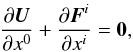 (1)where
 ![\begin{eqnarray} &&{\vec U} = \left(D,\,S_{\!\!j},\,\tau\right),\nonumber\\[4mm] &&\text{and}\; {\vec F}^i = \left(Dv^i,\,S_{\!\!j}v^i + p\delta^i_j,\,\tau v^i +pv^i\right). \end{eqnarray}](/articles/aa/full_html/2015/03/aa25182-14/aa25182-14-eq6.png) (2)In the case of an ideal gas, the conserved fluid variables U are defined in terms of the primitive fluid variables as
(2)In the case of an ideal gas, the conserved fluid variables U are defined in terms of the primitive fluid variables as 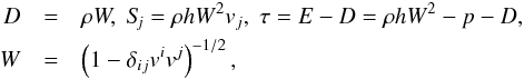 (3)where ρ is the fluid density, p is the pressure, vi is the velocity vector, and W is the Lorentz factor. The specific enthalpy h = h(ρ,p) characterises the heat content of a fluid per unit volume, and it defines the equation of state for the fluid when written as a function of the pressure and density. The conserved variables are the relativistic density D, the three-momentum Si, and the relativistic energy E, although we evolve τ, being the difference of the total relativistic energy and the relativistic density, in place of E to allow for more accurate evolutions as otherwise variations in p can be swamped by the relatively large relativistic density D, following Martí & Müller (2003).
Given an equation of state defined through the specific enthalpy h, the energy momentum tensor for a perfect fluid is given by 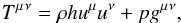 (4)where the four-velocity uμ is defined in terms of the three-velocity vi via
  (5)Here, W = (1 − vivi)− 1/2, calculated for Minkowski space-time. The specific enthalpy of an ideal fluid is
 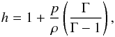 (6)where Γ (assumed to be constant) is the adiabatic index of the fluid (often written as γ, but this symbol is reserved for the determinant of the three-metric). The speed of sound in the fluid, cs, is then given by
  (7)In the case of non-relativistic ideal-gas, the recovery of the primitive variables from the conserved variables is an algebraic operation. However, for relativistic fluids the presence of the Lorentz factor complicates the issue, since the three-momentum components are no longer independent of each other, so we use a Newton-Raphson method to recover the primitive variables. Other techniques are available, including the solution of a quartic, but tend to be computationally involved and expensive. The Newton-Raphson approach we use follows the one given in Appendix A of Eulderink & Mellema (1995). We chose this over the approach of Martí & Müller (2003) as in our experience the latter appeared susceptible to numerical round-off errors when evaluating W, and appeared to lead to problems if the conserved variables had accumulated errors that took them outside the physically valid range. Eulderink & Mellema’s method, on the other hand, requires no calculation of W and, although it may be susceptible to issues of numerical precision, or lead to very small densities and pressure, we believe that we have rectified these in a robust fashion, as follows:
Given the conserved variables given above, we solve the following for ξ in order to recover the primitive variables:
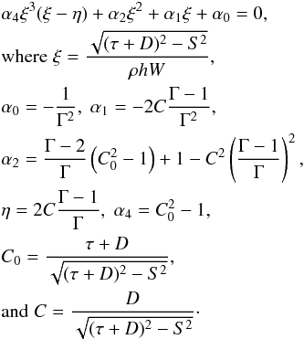
We note that, in order to retain numerical accuracy, the expression for calculating u0 = W in Eq. (A.12) of Eulderink & Mellema (1995) should be rewritten as 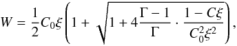 (9)taking C0ξ outside the brackets, since for large W the bracketed expression is of order unity and C0ξ is large. We then use the following to recover the remaining primitive variables:
  (10)where we have chosen ρmin = 10-8. Given that ρ may have been altered from its correct value of D/W, we recalculate the appropriate value of p from h, enforce p ≥ pmin if necessary, and then recalculate h before calculating vi as
  (11)According to Eulderink & Mellema (1995), “with some effort it may be shown that the derivative of [the quartic (8)] is always at least 2/Γ in its physical root, thus guaranteeing quadratic convergence for the Newton[-Raphson] method”. This gives us confidence that the approach is robust, and will remain so even when applied to more extreme flows, in cases where numerical errors are more likely, such as the evolution of a fluid on a strongly curved space-time metric.
3. HRSC schemes and MUSTA
Finite volume schemes (FV) are often used for the solution of equations in conservation-law form. The solution is approximated using averages over grid cells, and is advanced in time by the addition and subtraction of fluxes of the conserved quantities across the grid cell edges: 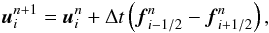 (12)where we have a grid-spacing Δx, a time-step Δt,
  is an approximation to the solution expressed in conserved variables in grid-cell i at time-step n, and
  is an approximation to the flux of conserved quantities between cells i − 1 and i at time-step n.
Since the finite volume approach is based on the integral form of the conservation law, it is suited to problems where discontinuities are expected. The sine qua non of finite-volume schemes is therefore the accurate approximation of the fluxes of the conserved quantities through the cell edges. The way in which the solution is updated using Eq. (12)ensures conservation, but care must be taken to ensure that no spurious oscillations arise in the vicinity of shocks.
A subset of finite volume schemes is the set of high-resolution shock-capturing (HRSC) schemes. These are capable of capturing shocks with very little smearing, even at low resolution, and are of at least second-order accuracy in smooth regions of the flow.
3.1. FORCE and SLIC schemes
One of the most basic FV schemes is the First ORder CEntred (FORCE) scheme. It can be applied to any set of PDEs in conservation form (omitting source terms) with little effort. The flux approximation is calculated as follows: ![\begin{eqnarray} &&{\vec f}_{i+\frac{1}{2}}^\mathrm{FORCE} \left({\vec u}_i^n, {\vec u}_{i+1}^n\right) = \frac{1}{2} {\vec f}_{i+\frac{1}{2}}^\mathrm{LW} + \frac{1}{2} {\vec f}_{i+\frac{1}{2}}^\mathrm{LF}\nonumber\\ &&\hspace*{5.3mm}=\frac{1}{2}{\vec f}_{i+\frac{1}{2}}^\mathrm{LW} + \frac{1}{4}\left[\left({\vec f}_i^n+{\vec f}_{i+1}^n\right)\right] +\frac{1}{4}\frac{\Delta x}{\Delta t}\left({\vec u}_i^n-{\vec u}_{i+1}^n\right),\nonumber\\ &&\text{where } {\vec f}_i^n={\vec f}({\vec u}_i^n),\;{\vec f}_{i+\frac{1}{2}}^\mathrm{LW} = {\vec f}\left({\vec u}_{i+\frac{1}{2}}^{n+\frac{1}{2}}\right),\nonumber\\ &&\text{and}\;{\vec u}_{i+\frac{1}{2}}^{n+\frac{1}{2}}=\frac{1}{2}\left({\vec u}_i^n+{\vec u}_{i+1}^n\right)+\frac{1}{2}\frac{\Delta t}{\Delta x}\left({\vec f}_i^n-{\vec f}_{i+1}^n\right). \end{eqnarray}](/articles/aa/full_html/2015/03/aa25182-14/aa25182-14-eq47.png) (13)
(13)
This is first-order accurate, and is a centred scheme, meaning that it does not have a (solution dependent) bias to information from either the left or the right. As will become relevant later, FORCE is the simple average of two other numerical schemes: the Lax-Wendroff scheme, being the term  , and the Lax-Friedrichs scheme, being the term
  . The Lax-Wendroff scheme is second-order but oscillatory, and the Lax-Friedrichs scheme is first-order, but very diffusive. It turns out that the FORCE scheme is the least diffusive non-oscillatory three-point first-order linear scheme that is not dependent on local solution information. The FORCE scheme is based on the piecewise constant reconstruction of the solution, i.e. the left and right states are taken directly from the solution vectors and
  .
.
One improvement over the constant piecewise reconstruction, known as the SLIC scheme (Slope-LImited Centred), is to use cells i − 1 and i + 2 to make a piecewise linear reconstruction of the solution at time n + 1/2 to provide initial states for the Riemann problem. However, we must take care that, in reconstructing the solution, we do not introduce any new extrema into the solution. We first reconstruct the slope of the solution, Δi, using data from either side of the current cell, taking the average of the forward and backward differences:  (14)and then determine a limited slope
  by multiplying each component by a factor dependent on the local solution behaviour:
 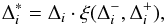 (15)where
 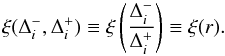 (16)The preceding two equations are applied to each individual component of Δi,
  , and
, and  to form the limited slope . The SLIC flux is then calculated as
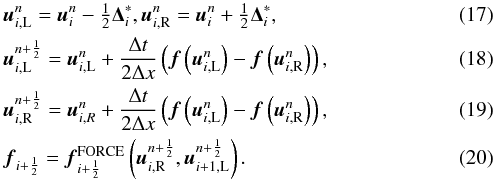 where we use
  and
and  as the left and right states for the FORCE flux.
There are many choices for the slope-limiter ξ, even given the constraint that the overall numerical scheme should be Total Variation Diminishing (TVD) as defined by Toro (1999). If we restrict the limiter to be a function of the ratio of the forward and backward differences: 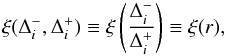 (21)then the constraints on ξ(r) can be shown to be (Toro 1999, p. 505, setting ω = 0): where
 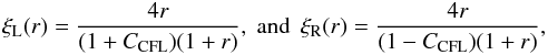 (22)with CCFL being the local Courant number.
We see that the ratio r is a measure of the change in slope around cell i. It is negative if i lies at an extremum of the solution, as one of  and
and  will be positive and the other negative, and this is the reason that we require ξ(r) = 0 for r< 0 as any non-constant reconstruction would result in an overshoot or undershoot of the extremum.
The slope-limiter that we will use in this paper is the van-Leer limiter given by: 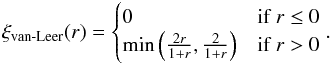 (23)This limiter is a good compromise between compressive (super-bee) and diffusive (min-mod) limiters, and we have found it suitable for our purposes, not leading to excessive smearing of shocks, nor any spurious oscillations.
3.2. MUlti-STAging approach (MUSTA)
When considering the accuracy of a numerical scheme, one must take into account both the order of accuracy (for example second-order in both space and time) and the “error-constant”. In other words, if the solution error is locally of the form  (24)then the accuracy depends both on p and q and also the constant ci. Thus the accuracy of the scheme can be improved by decreasing the error constant without decreasing the order of accuracy.
In order to improve on the accuracy of SLIC, we could consider Riemann solvers (as an alternative to FORCE to calculate the first-order solution) which use information about the wave types making up the solution to calculate the flux. These tend to be computationally intensive, often requiring iterative or matrix methods to determine the flux at the cell face. In order to increase the order of accuracy, we could use a higher-order reconstruction than the linear one that SLIC uses. Again, this would require more computational expense. However, Toro (2003) has suggested a simple way of improving the accuracy of any numerical scheme, which can produce improved accuracy for less computational effort than would be required if the accuracy were to be attained by increasing resolution. This is called MUSTA, which stands for MUlti-STAging and can be understood as follows.
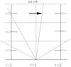 |
Fig. 1 How to multi-stage a simple numerical scheme (e.g. FORCE). The Riemann problem is solved for several time steps using the simple scheme on the two-cell domain, with transmissive boundary conditions as shown by the empty arrows. The solid lines show the wave structure of the solution. As the number of stages increases, the waves move away from the centre, so that the flux at the centre tends to the correct limit, which is represented by the filled arrow at the top. This figure corresponds to calculating the FORCE3 scheme, if FORCE is used as the underlying simple scheme. |
The FORCE flux provides a simple way of estimating the flux at a cell face. We can define an approximate Riemann solver by using the FORCE (or any other) flux to evaluate the initial flux and then seeking to correct it using multiple evaluations of the flux on the resulting solution, and using the resulting flux on the face to define an improved numerical flux for the original scheme. The MUSTA approach uses this idea to numerically evolve the Riemann problem on a two cell grid, using some appropriate scheme, for a few time-steps, or stages, and to take the central flux at the last stage as the estimate for the final flux. This is represented in Fig. 1. When using the FORCE scheme as the basis for MUSTA, the MUSTA algorithm can be written as the iterative scheme  where
where  and
and  give the initial conditions based on the original Riemann problem. This scheme uses the transmissive boundary conditions where the solution has zero derivative at the boundary.
The best improvements in accuracy for least computational expense are likely to be found when multi-staging is applied to as simple and appropriate scheme as possible. Therefore, in order to improve the accuracy of SLIC, we do not multi-stage SLIC itself, but rather multi-stage the FORCE scheme on which SLIC is based. We write the multi-staged FORCE scheme as FORCEk, where k is the number of stages, so that FORCE1 ≡ FORCE. This notation is as in Toro (2003) but differs from that in Toro & Titarev (2006).
Although the preceding explanation seems plausible enough, we can examine the theoretical effect of MUSTA for the linear advection equation. As mentioned in Sect. 3.1, the FORCE scheme can be expressed as  (28)with
  .
.
The local CFL number cL is derived from the local wave speed  and global time step Δt as
  (29)For linear advection, many numerical schemes with a stencil width of three can be written in the form (28)for some ω, which may depend on the solution. Therefore we can plot the dependence of ω on cL for various schemes, as in Fig. 2. The Godunov scheme corresponds to the choice
  , the FORCE scheme to
  , Lax-Wendroff to ω = 1, and Lax-Friedrichs to ω = 0. The Godunov scheme, based on the exact Riemann solution, falls on the curved line shown. This splits the diagram into two parts. Above the curve lie schemes that are oscillatory, and below it lie schemes that are non-oscillatory, but are more diffusive than the Godunov scheme. The first-order Godunov scheme is the least diffusive non-oscillatory linear first-order method for the linear advection equation. The FORCE scheme can therefore be seen to be the least diffusive non-oscillatory first-order method that does not depend on the local wave speed information given by cL.
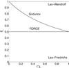 |
Fig. 2 Demonstration of how different first-order schemes for solving the linear-advection equation can be represented in the form 28 where ω depends on cL the local CFL condition. |
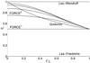 |
Fig. 3 Same as Fig. 2, with additional multi-staged versions of FORCE k where k = 1...5 and k increases up the page (labels for k = 3,4,5 are omitted for reasons of clarity). |
Although the MUSTA approach does not depend explicitly on cL, it does depend on it implicitly, through its dependence on the local data for the predictor step (25). This dependence can be calculated in a straightforward, but algebraically intensive manner, which we have done using Maple, and we plot the results for FORCE n, n = 1,..., 5 in Fig. 3. It is immediately clear that MUSTA may not be a suitable evolution scheme at high CFL numbers, even for linear advection, as all of the schemes now protrude into the oscillatory region. Using very high numbers of stages shows that FORCEk tends to the Lax-Wendroff scheme as k → ∞ (except for cL = 1 where for all k, so that the convergence is not uniform).
3.3. Generalised FORCE flux
The impetus for the development of MUSTA was the fact that even for the simplest of all conservation laws, the linear advection equation, the FORCE method was more diffusive than the Godunov scheme using the exact Riemann solver for CFL less than unity, and the approach was to improve the accuracy of a scheme, without requiring local wave speed information. However, we have seen that the MUSTA approach is not ideal as it can lead to oscillatory methods, even for linear advection.
Toro & Titarev (2006) presented a solution to this in the same paper as their MUSTA approach. In that paper, they calculate the generalised FORCE flux (GFORCE) as a weighted average of the Lax-Friedrichs and Lax-Wendroff fluxes, now dependent on local wave speed information: 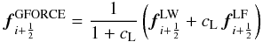 (30)where cL is the local CFL number, derived from the local wave speed and global time step Δt as
  (31)With these definitions, GFORCE replicates the Godunov upwind scheme for the linear-advection case. This suggests that the GFORCE flux could well provide improved accuracy for more complex systems of equations.
We note that the SR wave speeds in one dimension are given by 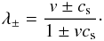 (32)As the GFORCE scheme already coincides with the Godunov scheme for the linear advection equation, applying the MUSTA approach makes no difference in this case, simply maintaining the Godunov scheme. However, this is not the case for more complicated systems of equations, which have multiple wave-speeds, and we shall see that multi-staging GFORCE provides some increase in accuracy.
3.4. HLL flux
The GFORCE flux, being equivalent to the flux from the first-order Godunov solver in this case, is the most accurate non-oscillatory first-order scheme for the linear advection equation. However, more complex systems of equations have more complex solutions to their Riemann problems. It is possible, in many cases, to derive a linearised or exact Riemann solver for a system of equations. However, this will usually involve either calculating a matrix inverse or using an iterative method to find the flux. This tends to be computationally expensive, and is therefore often avoided unless the pay-off of computational time versus accuracy is worthwhile.
However, a simple Riemann solver, applicable to any system of equations, was suggested by Harten et al. (1983), and is known as the HLL Riemann solver. The rationale behind this approach is that if all the waves in the solution are moving in one direction only, then the flux is taken wholly from one side or the other, and an appropriately weighted average is taken otherwise: 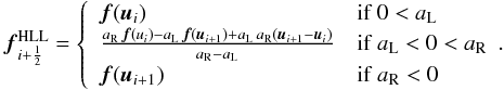 This is only dependent on approximations to the left and right local wave speeds aL and aR. These can be calculated from the fluid variables as suggested by Schneider et al. (1993)
 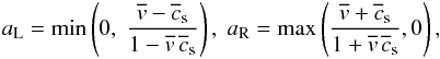 (33)where
  and
and  are the arithmetic means of the initial velocities and sound speeds in cells i and i + 1.
In the case of a curvilinear grid, we note that we have to transform the variables into the computational grid’s local coordinate system in order to find the wave speed parallel to the grid coordinate direction. We elaborate on this in Sect. 5.
3.5. Recommendations for the MUSTA approach
In summary, therefore, the multi-staging approach at first sight appears to produce a straightforward and cheap way of improving the accuracy of a simple flux approximation scheme. However, some investigation shows that applying it to the FORCE scheme alone may not be a viable approach as FORCE for k> 1 are oscillatory schemes for linear advection. An improvement on this appears to be to apply it to the GFORCE scheme, where GFORCE is not oscillatory for linear advection. Likewise, the HLL schemes are not oscillatory.
However, as the analysis has not been extended to more complex systems of equations, our recommendations are as follows: use of FORCE may be advantageous in that it captures peaks and discontinuities with less diffusion as k increases, but this method should be used with care since for k> 1 the scheme no longer satisfies the TVD property for the linear advection equation as illustrated in Fig. 3. Without further analysis the GFORCE and HLL schemes should also be used with caution although they are likely more robust than the FORCE scheme. The use of GFORCEk or HLLk does not, as yet, have any evidence of causing the loss of the TVD property although, given the analysis for FORCE, we suggest caution as to whether this result can be applied to more complex systems of equations.
We attach a caveat emptor here, therefore, to any use of multi-staging, but suggest that it may be useful if used with care, and with only a few extra stages, perhaps around three or so. We present some numerical results and comparisons in Sect. 6. In particular, the examples shown in Fig. 7 show the effect of increasing the multi-staging parameter.
In terms of a comparison to using an exact or approximate Riemann solver, the relative accuracy will depend on the system being solved. We have not made any direct comparisons with a Riemann-solver-based method, but in general centred schemes tend to smear contact discontinuities substantially more than Riemann solvers designed to capture these exactly. However, other regions of the flow should be captured with similar accuracy if sufficient MUSTA stages are used.
The MUSTA approach permits improved accuracy on top of that provided by FORCE by the simple addition of an extra containing loop within a single flux calculation. No further algebraic derivations are required as for a Riemann solver, and neither are any higher-order reconstructions, such as those required by CENO (Del Zanna & Bucciantini 2002). As demonstrated by Eulderink & Mellema (1995), constructing a Riemann solver takes substantial work.
Therefore, the advantage of our aproach is that it only requires the system fluxes and maximum wave-speeds to be specified, and affords an easy way of improving accuracy with minimal time penalty, without having to derive, implement, and test a full Riemann solver.
In terms of computational cost, we have not made a comparison with a relativistic Riemann solver. However, a comparison between FORCE and an exact Riemann solver for an ideal Eulerian gas in one dimension suggested that FORCE took about a third of the time, FORCE
 about two-thirds of the time, and FORCE
 about the same time. We would expect that for SRHD, the Riemann solver would take comparatively substantially longer than this, and so the performance gain would be far greater.
4. Overture
Overture1 is an infrastructure that supports the development of PDE solvers for overlapping curvilinear grids, as described by Brown et al. (1997). Overture includes support for grid generation, for individual component grids, and for generating the overlapping grid, and associated connectivity information required for interpolation. Users of Overture may utilise existing PDE solvers or implement their own approximations.
Our main reason for using Overture is that we wish to capture a spherical geometry, with a smooth inner excision boundary, so that we can include general relativistic effects and ultimately simulate fluid flow into a black hole. Relevant results for the GRHD equations will be presented in a future paper.
There are two main issues with regard to dealing with overlapping grids. The first is that of constructing the full grid structure. This is one of the tasks that Overture has been designed to perform even for very complicated grids. Given a set of logically rectangular grids, along with mappings to the physical grid coordinates, as well as boundary conditions, Overture can remove parts of grids that are obscured by other grids and calculate which cells on which grids should be used to interpolate data onto grid cells that are now near to cut-out portions of the grid.
In order to interpolate solution variables between grids, we have used polynomial interpolation. Overture uses Lagrange polynomials for interpolation, and takes into account the grid geometries involved. One potential drawback of using Lagrange polynomials is that, except for the linear case, it is not guaranteed that the interpolated values will be contained in the same range as the values from which they are interpolated. This could lead to overshoots developing near interpolation boundaries. However, although monotonicity preserving interpolation schemes can be derived, it was not found that the extra expense was worthwhile.
We used a fifth-order accurate interpolation, based on a five-point stencil, which required two lines of interpolation points at the edge of each grid. We required two lines of interpolation points as the slope-limiting methods we use require two ghost cells at the grid boundaries.
5. Curvilinear grids
When solving a PDE on overlapping grids, each with its own curvilinear coordinate system, it is usual to transform the governing equations to the new grid coordinate systems but retain the Cartesian components of the dependent variables. This simplifies interpolation between different component grids.
The curvilinear grid is defined by a smooth transformation, xi = φ(ri), from Cartesian coordinates xi to the unit square parameter space coordinates ri. This means that we transform the governing equations as follows 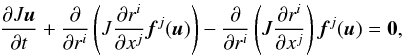 (34)where J is the Jacobian of the transformation:
 ![\begin{eqnarray} J = \left|\left[\frac{\partial x^i}{\partial r^j}\right] \right|\cdot \label{eqn:Jacobian} \end{eqnarray}](/articles/aa/full_html/2015/03/aa25182-14/aa25182-14-eq124.png) (35)The third term in Eq. (34)is added so that at the discrete level we maintain the geometric conservation law (this is also known as free-stream preservation). When the flux is not spatially dependent, the second term in Eq. (34)is zero analytically, but may not be zero when evaluated numerically. The third term is added to ensure that, when the flux is constant spatially, the flow remains constant. The term is composed of an evaluation of f on a cell-centred value of u, multiplied by a geometric term. This geometric term must be calculated in a manner consistent with the second term, so that, for a constant state u, the geometric terms will cancel exactly (at least up to round-off error).
(35)The third term in Eq. (34)is added so that at the discrete level we maintain the geometric conservation law (this is also known as free-stream preservation). When the flux is not spatially dependent, the second term in Eq. (34)is zero analytically, but may not be zero when evaluated numerically. The third term is added to ensure that, when the flux is constant spatially, the flow remains constant. The term is composed of an evaluation of f on a cell-centred value of u, multiplied by a geometric term. This geometric term must be calculated in a manner consistent with the second term, so that, for a constant state u, the geometric terms will cancel exactly (at least up to round-off error).
The process of evaluating the third term is fairly straightforward in practice. For any given HRSC scheme, we can do this by starting with a fluid with constant density, velocity, and pressure, and compute the fluxes analytically, ensuring that the flow is preserved, regardless of the geometry or other parameters, such as slope-limiter. In the case of SLIC, the result is that the flux for each cell face is composed of the product of a flux, derived from the given constant state, and a geometry term of the form  . Since the final flux for a given coordinate direction ri is then simply a difference of these, the term that cancels these is
 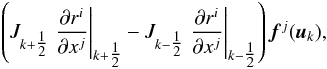 (36)where the values of the Jacobian and coordinate derivatives have to be calculated in exactly the same way as in the rest of the HRSC scheme being used.
5.1. Curvilinear SLIC scheme
The SLIC scheme requires the reconstruction of states at cell-faces. We have changed the SLIC algorithm slightly to take account of the spatial of the Jacobian on curvilinear grids.
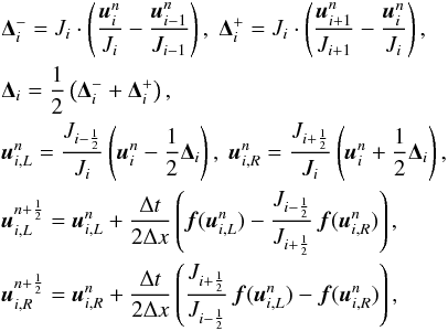 (37)where Ji is the Jacobian of cell i, and
  . The derivatives ∂ri/∂xj, however, are averaged differently since, in one dimension, we know that J-1 = ∂r/∂x, and so we want to ensure that
 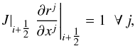 (38)where there is no sum over j.
One way to ensure that this is always true is to average the derivatives of the inverse mapping using the harmonic mean 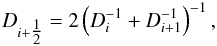 (39)where the matrix Di is defined as
 ![\begin{eqnarray} D_i = \left.\left[\frac{\partial r^l}{\partial x^m}\right]\right|_{x=x_i}\cdot \end{eqnarray}](/articles/aa/full_html/2015/03/aa25182-14/aa25182-14-eq138.png) (40)Even in the case of multi-dimensions, we never need to calculate the fluxes across more than one cell-face at a time, so the above averaging is only ever done in one computational grid direction.
(40)Even in the case of multi-dimensions, we never need to calculate the fluxes across more than one cell-face at a time, so the above averaging is only ever done in one computational grid direction.
5.2. HLL flux
In order to calculate the HLL flux in curvilinear coordinates, we first transform the Cartesian components of the solution variables into the local grid coordinate basis. The wave speeds are then calculated for the required coordinate direction from the transformed variables. In the same way as SLIC, we calculate the fluxes in the local grid coordinate direction, multiplied by the local Jacobian. In order to achieve second order convergence, we adjust the HLL flux to read: 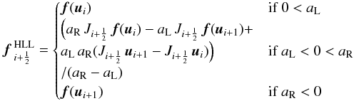 (41)where the fluxes are calculated parallel to the local grid coordinate i. We note that the local CFL number defined in Eq. (31)required for the calculation of GFORCE is also derived from the wave speeds calculated along the local grid coordinate directions.
5.3. Determination of the time-step
On Cartesian grids, the maximum time-step that retains stability for the SLIC scheme is given by  (42)where CCFL ≤ 1 is the CFL number, Δx is the grid spacing, and Smax is the maximum wave-speed, obtained from (32). On curvilinear grids, we determine the global time-step as the minimum of local time-steps determined on a cell-by-cell basis, where Δx is chosen appropriately from the local cell size. The alternative, taking the minimum cell size and the maximum wave speed over the whole grid, can lead to time steps that are more restrictive than necessary. Further, when we wish to calculate the wave-speeds, we in fact transform the numerical solution into the local grid basis so that the correct wave speeds along the coordinate directions can be found, as these may not be aligned with Cartesian directions, which could lead to an underestimate of the local wavespeed.
However, a draw-back of using curvilinear grids is that the cells are not of similar size everywhere. Even with the above method of calculating the time-step, this still leads to an effectively lower CFL number for evolution on larger grid cells, as the time-step has been restricted by the stability condition on smaller grid cells. Therefore waves may become somewhat smeared on a coarser area of the grid only because of finer resolution elsewhere.
We can reduce the effect of this problem by using as accurate a scheme as possible, namely GFORCE or HLL, which provide accurate solutions even at lower CFL numbers.
6. One-dimensional test problems
In order to test the stability and accuracy of the GFORCE scheme and the MUSTA approach, we have applied them to some standard one-dimensional test-cases which have been used previously in the literature. The tests we consider are carried out using a one-dimensional uniform resolution code using the same numerical schemes as the Overture code, but without the overhead imposed by Overture.
An exact solution to the Riemann problem for the one-dimensional special relativistic hydrodynamical equations exists, and so we can compare our numerical results to this. In order to generate the exact solutions, we have used the code riemann.f from Martí & Müller (2003).
The test-cases we use are taken from Del Zanna & Bucciantini (2002), so that a comparison can be made with their numerical results, which were obtained using a Convex ENO reconstruction and the HLL Riemann solver. The three test-cases below all use an ideal fluid with adiabatic index Γ = 5/3 and are performed on a domain of x ∈ [0,1].
6.1. Mildly relativistic shock
The initial conditions for this test are ![\begin{eqnarray} (\rho,\;v,\;p) = \left\{\begin{array}{ll} (10,\;0,\;13.3)&\text{ if } x < \frac{1}{2} \\[1mm] (1,\;0,\;0) &\text{ if } x > \frac{1}{2}\cdot \end{array}\right. \label{eqn:MildShock} \end{eqnarray}](/articles/aa/full_html/2015/03/aa25182-14/aa25182-14-eq145.png) (43)It is fairly easy to obtain good results for this test, as it contains no extreme velocities or densities. The solution is evolved to a time t = 0.4. It has been noticed by other researchers (e.g. Del Zanna & Bucciantini 2002) that, for certain schemes, the initial zero pressure has to be set to some small non-zero value. We use a minimum pressure of pmin = 10-8, assuming reference pressures of order 1.
(43)It is fairly easy to obtain good results for this test, as it contains no extreme velocities or densities. The solution is evolved to a time t = 0.4. It has been noticed by other researchers (e.g. Del Zanna & Bucciantini 2002) that, for certain schemes, the initial zero pressure has to be set to some small non-zero value. We use a minimum pressure of pmin = 10-8, assuming reference pressures of order 1.
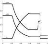 |
Fig. 4 Results for a mildly relativistic shock wave, (ρ,u,p)L = (10, 0, 13.3) and (ρ,u,p)R = (1, 0, 0), using 400 cells, a CFL number of 0.99, and the van Leer limiter, with the SLIC scheme based on the GFORCE3 flux, simulated to time t = 0.4. The exact solution is given by the solid line and is composed of a rarefaction, a contact discontinuity, and a shock. |
An example result is shown in Fig. 4 using the SLIC scheme with the van Leer slope limiter, based upon the GFORCE 3 scheme, and using a CFL number of 0.99. The right-most discontinuity, corresponding to a shock wave, is captured with only four points. In this, and in the capturing of other discontinuities, we see that our results are as good as those of Del Zanna & Bucciantini (2002). However, the capturing of the density is seen to be somewhat better in Lucas-Serrano et al. (2004). We also note that the kink we find in the velocity at x ≈ 0.6 (near where the solution has a discontinuity in the slope) is present to a slightly lesser extent in Lucas-Serrano et al. (2004), and not at all in Del Zanna & Bucciantini (2002).
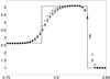 |
Fig. 5 Results for the density of a mildly relativistic shock wave, (ρ,u,p)L = (10, 0, 13.3) and (ρ,u,p)R = (1, 0, 0), using 400 cells, a CFL number of 0.99, and the van Leer limiter, with the SLIC scheme based on the fluxes: FORCE (circles), GFORCE (squares), GFORCE3 (crosses), and HLL (+ signs). The exact solution is given by the straight line. We restrict the region plotted so that the differences between the methods can be seen. |
Figure 5 shows the result near the leading shock using four different numerical schemes for the same problem. All the methods use the SLIC scheme, based on four different fluxes: FORCE, GFORCE, GFORCE3, and HLL. It can be seen that there is very little difference indeed between the methods. This is due to the mild nature of the problem. However, we can make the differences between the methods more apparent by evaluating the ℒ1 error of the density for each of several methods, using a range of CFL numbers. The results are shown in Table 1. The error norm is taken over the whole domain and so includes the discontinuities. We see that increasing the number of stages used for a scheme reduces the error. In all cases, the GFORCE scheme is better than the FORCE scheme, although the FORCE2 scheme is always better than the GFORCE2 scheme, except for the case of CCFL = 0.4, where the numerical evolution blows up. We note this data as evidence for the caveat emptor in Sect. 3.5. The reason for the improvement of FORCE k over GFORCE is that the FORCE k scheme is usually above the GFORCE scheme as shown in Fig. 3, as a result of its lessening diffusion at the expense of potentially introducing oscillations into the solution. The GFORCE scheme is of similar accuracy to the HLL scheme, although it is slightly worse at CFL 0.4. There is a slight improvement in accuracy when increasing the number of stages used for the GFORCE scheme. We also note that the error decreases for higher CFL numbers, both as a result of the reduced number of time-steps required to reach the final time and the fact that schemes are often more accurate for CFL numbers close to 1.
However, in general, the FORCE and GFORCE schemes are more accurate than the HLL scheme, at least for k ≥ 2. This is roughly in line with what we would expect from the analysis of the various schemes on the linear advection equation in Sect. 3.
Error norms of the density using ∥ ·∥ 1 for various base schemes for the SLIC method applied to the mildly relativistic shock test.
6.2. Strongly relativistic Blast-Wave
The initial data for this problem is given by ![\begin{eqnarray} (\rho,\;v,\;p) = \left\{\begin{array}{ll} (1,\;0,\;1000)&\text{ if } x < \frac{1}{2}\\[1mm] (1,\;0,\;0.01) &\text{ if } x > \frac{1}{2}\cdot \end{array}\right. \label{eqn:BlastWave} \end{eqnarray}](/articles/aa/full_html/2015/03/aa25182-14/aa25182-14-eq191.png) (44)This is a more difficult test-case to evolve, as the solution contains a narrow peak of high density, which is hard to capture at low resolution, and also contains velocities which approach c = 1. This problem is also evolved to a time t = 0.4. The exact solution for all variables is shown as part of Fig. 6. This shows a narrow region of high density moving close to the speed of light. The maximum density is very difficult to capture at a moderate resolution such as we are using due to the narrowness of the peak. A good test of the accuracy of a scheme, therefore, is the fraction of the peak value that is attained.
(44)This is a more difficult test-case to evolve, as the solution contains a narrow peak of high density, which is hard to capture at low resolution, and also contains velocities which approach c = 1. This problem is also evolved to a time t = 0.4. The exact solution for all variables is shown as part of Fig. 6. This shows a narrow region of high density moving close to the speed of light. The maximum density is very difficult to capture at a moderate resolution such as we are using due to the narrowness of the peak. A good test of the accuracy of a scheme, therefore, is the fraction of the peak value that is attained.
An example result, obtained using the SLIC scheme based on GFORCE, using the van Leer limiter, with a CFL of 0.99, and using 400 cells, is shown in Fig. 6. The solution is already quite accurate, and the density peak is at 65.6% of its correct value. Del Zanna & Bucciantini (2002) achieved peaks of 70.1% and 62.4% for two different versions of their method, and Lucas-Serrano et al. (2004) attained a density peak of 76% of the exact value (the comparison is not quite valid as Del Zanna & Bucciantini (2002) only evolved to time t = 0.35, rather than t = 0.4 as used here and in Lucas-Serrano et al. 2004).
On comparing different underlying first-order methods for SLIC, we find that once again there is little visual difference between the results, and we therefore give the density peaks in Table 2. These results are in line with what we have already seen, that FORCE k tends to be more accurate than GFORCE k for k ≥ 2, and that HLL is more accurate than GFORCE when no multi-staging is used.
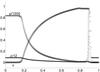 |
Fig. 6 Results for the blast-wave Riemann problem given by (44)using 400 cells, a CFL number of 0.99, and the van Leer limiter, with the SLIC scheme based on the GFORCE flux, to time t = 0.4. The exact solution is given by the solid lines, and is composed of a rarefaction, a contact discontinuity, and a shock. The maximum velocity is v ≈ 0.960, corresponding to a Lorentz factor of 3.59. Numerical results are given for pressure (squares), velocity (circles), and density (crosses), all scaled by appropriate factors to fit them all onto one plot. |
In Table 3 we give the ℒ1 errors in the density for various resolutions and methods. This shows near first-order accuracy over the whole problem, which is the best that we can expect for a solution containing discontinuities.
Density peak for strongly relativistic shock as predicted by various methods at a resolution of 400 cells.
ℒ1 norm errors in density for the blast-wave test, evaluated over the whole domain.
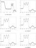 |
Fig. 7 Results for the density-perturbation initial conditions. The first plot shows a full solution obtained using the SLIC scheme based on FORCE1. The other plots show close-ups of the density when replacing FORCE by other schemes. For all results, a CFL of 0.99 and the van Leer limiter were used, on a grid of 400 cells. |
6.3. Perturbed density test
The initial data for this problem is given by ![\begin{eqnarray} (\rho,\;v,\;p) = \left\{\begin{array}{ll} (5,\;0,\;50)&\text{ if } x < \frac{1}{2}\\[1mm] (2+0.3\,\sin(50x),\;0,\;5) &\text{ if } x > \frac{1}{2}\cdot \end{array} \right. \label{eqn:PerturbedDensity} \end{eqnarray}](/articles/aa/full_html/2015/03/aa25182-14/aa25182-14-eq209.png) (45)This problem provides a good indicator of how well a numerical method can capture extrema. There is no analytic solution to this, and instead we use a converged numerical solution, generated at high-resolution. This test is evolved to t = 0.35, since the results of Del Zanna & Bucciantini (2002) are consistent with this, not t = 0.4 as stated in their main text. The converged solution, evolved using the SLIC 1 scheme with van Leer limiter, and 20 000 cells, is shown as the first part of Fig. 7. We note that this is visually indistinguishable from the result using 10 000 cells. Superimposed on this is an example evolution, using 400 cells and the SLIC scheme based on FORCE. Points to note are that the three sharp peaks are not particularly well captured, and that the final peak at the right of the figure is clipped. We note that Del Zanna & Bucciantini (2002) manage to capture the peaks somewhat better than we do whilst using half the number of cells.
(45)This problem provides a good indicator of how well a numerical method can capture extrema. There is no analytic solution to this, and instead we use a converged numerical solution, generated at high-resolution. This test is evolved to t = 0.35, since the results of Del Zanna & Bucciantini (2002) are consistent with this, not t = 0.4 as stated in their main text. The converged solution, evolved using the SLIC 1 scheme with van Leer limiter, and 20 000 cells, is shown as the first part of Fig. 7. We note that this is visually indistinguishable from the result using 10 000 cells. Superimposed on this is an example evolution, using 400 cells and the SLIC scheme based on FORCE. Points to note are that the three sharp peaks are not particularly well captured, and that the final peak at the right of the figure is clipped. We note that Del Zanna & Bucciantini (2002) manage to capture the peaks somewhat better than we do whilst using half the number of cells.
The rest of Fig. 7 shows the results for various schemes, focusing on the region 0.6 ≤ x ≤ 1. Now we see that increasing the number of stages used improves the capturing of the three peaks and the knees at x ≈ 0.7 and x ≈ 0.85. The ordering of the plots has been chosen to show a progressively increase in accuracy. We see that multi-staging GFORCE out-performs HLL, and that multi-staged FORCE still produces better accuracy than multi-staged GFORCE. However, in our experience, multi-staged FORCE appears to be more robust, and we note that although increasing multi-staging generally improves accuracy, the pay-off after about three stages is small relative to the extra computational cost.
7. Validation in two spatial dimensions
In this section we give details of various validation tests we have carried out in two spatial dimensions, making use of the overlapping grid capabilities of our algorithm.
7.1. One-dimensional shock across overlapping grids
It is important to test the accuracy of the method on curvilinear, overlapping grids since use of these grids will be integral to our later work. To this end, we evolve a one-dimensional Riemann problem with a known solution across the two-dimensional domain, with outer vertices at (± 0.5, ± 0.5) shown in Fig. 8, where the Cartesian grid has resolution 400 × 400, and the annulus matches its resolution to that of the Cartesian grid at its inner circumference. This is designed to test the accuracy of the interpolation between a curvilinear grid and a regular Cartesian grid, as well as the accuracy of the evolution taking place on an annular geometry, rather than a Cartesian grid. From a physical point of view, this is just evolving the shock-test on a square domain, but the presence of the embedded curvilinear grid adds numerical and algorithmic complexity. As initial conditions we use the Riemann problem 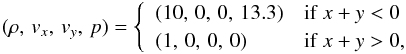 (46)so that the shock is propagating diagonally across the grid.
As this is only a 1D test evolved on a 2D grid, the exact solution can be found as in Sect. 6. We perform the evolution using the grid described in Fig. 8, and sample the solution at 400 points (corresponding to the Cartesian grid’s resolution) along the line x = y, perpendicular to the shock direction, at a time of t = 0.4. Figure 9 shows the results from using the GFORCE flux, with a CFL of 0.95 and the van Leer limiter. We can see that the solutions on the plain 2D Cartesian grid and on the overlapping grid are almost indistinguishable.
7.2. The two-dimensional Riemann problem
We can also test the multi-dimensionalisation of our schemes in a simple two-dimensional test, essentially a two-dimensional Riemann problem. Due to the two-dimensional nature of the set-up, there is no known exact solution to this problem, but we can compare our results to those of other authors such as Del Zanna & Bucciantini (2002). The problem is defined on a region [0,1] × [0,1] and is evolved to a time t = 0.4, with initial conditions 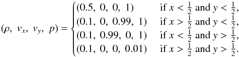 (47)This setup is symmetric about the line x = y, so that the evolved solution should maintain this symmetry.
Figure 10 shows the results for two different schemes, FORCE and GFORCE, both using the van Leer limiter. The resolution used is 400 cells in each direction, using a CFL of 0.95. Although there is no exact solution for this initial data, the results compare well with those of Del Zanna & Bucciantini (2002), in that the same features are captured, and with similar widths. We note that the long density peak in the upper-right of the figure is more pronounced in our scheme than in Del Zanna & Bucciantini (2002), but that the feature just below and to the left of the centre is somewhat less well-defined in our plot than in Del Zanna & Bucciantini (2002). It is in fact the case that, within this region, the density drops to a very small value indeed, of the order of 10-6. It is also the case, although not entirely clear on the plots shown, that the discontinuities are slightly narrower for the GFORCE scheme than for the FORCE scheme.
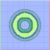 |
Fig. 8 Grid for testing curvilinear and overlapping routines. An annulus is superimposed on a Cartesian grid and used to replace part of that grid. The Cartesian grid has its vertices at (± 0.5, ± 0.5), a resolution of 400 × 400, and the annulus resolution matches that of the Cartesian grid at the inner circumference. We only show every fourth gridline in this plot for clarity. |
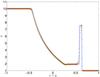 |
Fig. 9 Cross-section of the evolution of the mildly relativistic shock-wave across the grid shown in Fig. 8. The run was performed using the GFORCE1 scheme at a CFL of 0.95, and using the van Leer slope-limiter. The green + signs are the numerical solution on the overlapping grid, the red circles are from an equivalent simulation on a single 2D Cartesian grid, and the blue line is the exact solution for the problem. The two numerical solutions have been interpolated from along the line x = y. |
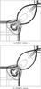 |
Fig. 10 Quadrants problem evolved at a resolution of 400 × 400, with a CFL of 0.95, using the FORCE1 and GFORCE1 schemes with the van Leer slope-limiter. We plot the log of the density ρ, using 30 equally spaced contours from ln0.1 = −2.303 to ln3.927 = 1.368. |
7.3. Front-facing step
In order to demonstrate the overlapping grid approach, we apply our code to the problem of a fluid shock forming ahead of a solid front-facing step, similar to the one presented in Lucas-Serrano et al. (2004). Since this benchmark has a grid-aligned geometry, it can be performed with far simpler mesh-generation approaches, such as by a block-structured methodology based on orthogonal cells. In order to demonstrate the versatility of Overture, we smooth the corner of the step, as shown in Fig. 11. The fluid has an initial density of 1.4, with an adiabatic index of 1.4. The fluid is initially steady, and the left-hand boundary has an inflow of fluid at velocity vx = 0.8, at Mach 3, and the system is evolved to time t = 10.
The resulting flow pattern is shown in Fig. 12, where we plot iso-contours of the log of the density. This compares qualitatively well to the results of Lucas-Serrano et al. (2004).
7.4. Reflective cylinder
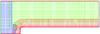 |
Fig. 11 Grid used for the front-facing step problem. The grid is made up of three separate grids: one for the incoming channel, one for the rest of the channel, and one for the step itself. The last has stretched grid cells that become narrower towards the edge of the step. For clarity we only show every other grid line. |
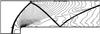 |
Fig. 12 Solution at t = 10 for a shock hitting a front-facing step. The fluid has adiabatic index Γ = 1.4, velocity v = 0.8 and is travelling at Mach 3. The scheme used was GFORCE1 with the van Leer slope-limiter, and with CFL 0.95. We plot 30 contours of the log of the density. |
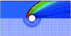 |
Fig. 13 Solution for a reflective cylinder initially immersed in a constant velocity flow of Mach 3, velocity 0.8, adiabatic index Γ = 1.4, and density 1.4. The main channel has length 10 and width 5, composed of 100 × 200 cells. The annulus has inner radius 0.5 and outer radius 1.25, with 168 cells in the angular dimension, and 32 cells in the radial direction, where an exponential stretching function has been applied in the radial direction to restrict the radial size of cells nearer the inner boundary. For clarity, we only show every other grid line. In the top half of the plot, contours of ρ at time t = 10 are shown. The scheme used was GFORCE1, with the van Leer slope-limiter, at a CFL of 0.95. There are 30 contours, equally spaced between 0 and 10. |
Since we intend to apply this code to problems in general relativity, we demonstrate a problem that is somewhat similar in its grid setup and initial conditions to that of a fluid impacting on a black hole. In this problem, we immerse a solid cylinder in a constant velocity flow and allow the numerical solution to evolve to steady-state. This general setup has been much studied in the non-relativistic case, and we expect to see qualitatively similar results here. Our grid is constructed from a Cartesian grid for the channel of size 10 by 5, containing an annulus with inner radius 0.5, the inner circumference of which is a reflective boundary. The channel’s walls are given transmissive boundary conditions, with the exception of the left boundary, which is an inflow boundary. The grid is shown in the bottom half of Fig. 13. The state of the simulation at time t = 10 is shown in Fig. 13. The solution consists of a strong bow shock in front of the cylinder, and there is some evidence of an unstable wake beginning to form downstream, as would be expected. The solution has qualitatively similar characteristics to those exhibited by the non-relativistic problem.
7.5. Multiple reflective cylinders
In Fig. 14 we show an extension of the problem from the previous section, to the case where there is more than one reflective cylinder in the domain. The same constant state initial data was used, this time incoming from the right. Since the numerical solver we developed can handle general overlapping grids, it was relatively simple to go from the single cylinder case to the multiple cylinder case. We show both the grid as used by Overture and the result which, while it cannot be validated, demonstrates qualitatively plausible behaviour.
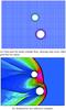 |
Fig. 14 Simulation of flow past two solid cylinders. The first plot shows the grid and in the second we plot 30 contours of ρ from 0 to 10 for two solid cylinders initially immersed in a fluid of constant state, Mach 3 and velocity 0.8, with density 1.4 and adiabatic index 1.4. The solution is shown at time 10. The GFORCE1 scheme was used, with the van Leer slope-limiter, and a CFL of 0.95. |
8. Conclusions and further work
In this paper, we developed a numerical scheme to solve the SRHD equations in complex geometries. The approach was based on the second-order SLIC method, with fluxes obtained through the MUSTA approach applied to the FORCE and GFORCE schemes. The properties of these new schemes were analysed and it was shown that the MUSTA approach can lead to more accurate results potentially at the cost of being less robust, although in practice the GFORCE scheme coupled with MUSTA presented no difficulties. The new schemes were then compared to each other and to the HLL scheme when applied to a number of one-dimensional test problems. We found that the MUSTA approach applied to the GFORCE scheme generally gave more accurate results than the HLL scheme. The scheme was then applied to a number of two dimensional problems using overlapping grids, which demonstrated the flexibility of the scheme to handle complex geometries.
In a future paper, we shall therefore extend our scheme to evolve general relativistic hydrodynamical problems, and present the way that we have adapted the numerical schemes presented in this paper to allow for a non-flat metric. It is our intention to apply our code to problems involving a stationary black-hole metric, in particular, to Bondi-Hoyle-Lyttleton accretion onto a Kerr black hole.
Freely available from http://www.overtureframework.org
Acknowledgments
This work was funded by an EPSRC Doctoral Training Grant. The authors would like to thank Eleuterio Toro for comments on the implementation of the MUSTA approach.
References
- Brown, D. L., Chesshire, G. S., Henshaw, W. D., & Quinlan, D. J. 1997, in Proc. of the Eighth SIAM Conf. on Parallel Processing for Scientific Computing [Google Scholar]
- Del Zanna, L., & Bucciantini, N. 2002, A&A, 390, 1177 [NASA ADS] [CrossRef] [EDP Sciences] [Google Scholar]
- Eulderink, F., & Mellema, G. 1995, A&AS, 110, 587 [NASA ADS] [Google Scholar]
- Harten, A., Lax, P. D., & van Leer, B. 1983, SIAM Rev., 25, 35 [Google Scholar]
- Lucas-Serrano, A., Font, J., Ibáñez, J., & Martí, J. 2004, A&A, 428, 703 [NASA ADS] [CrossRef] [EDP Sciences] [Google Scholar]
- Martí, J. M., & Müller, E. 2003, Liv. Rev. Rel., 6, 7 [Google Scholar]
- Rosswog, S. 2010, Class. Quant. Grav., 27, 114108 [NASA ADS] [CrossRef] [Google Scholar]
- Sanders, R. H., & Prendergast, K. H. 1974, ApJ, 188, 489 [NASA ADS] [CrossRef] [Google Scholar]
- Schneider, V., Katscher, V., Rischke, D., et al. 1993, J. Comput. Phys., 105, 92 [NASA ADS] [CrossRef] [MathSciNet] [Google Scholar]
- Toro, E. 1999, Riemann solvers and numerical methods for fluid dynamics, 2nd edn. (Springer-Verlag) [Google Scholar]
- Toro, E. 2003, Multi-stage predictor-corrector fluxes for hyperbolic equations http://www.newton.cam.ac.uk/preprints/NI03037.pdf [Google Scholar]
- Toro, E., & Titarev, V. 2006, J. Comput. Phys., 216, 403 [NASA ADS] [CrossRef] [Google Scholar]
- van Putten, M. H. P. M. 1993, ApJ, 408, L21 [NASA ADS] [CrossRef] [Google Scholar]
All Tables
Error norms of the density using ∥ ·∥ 1 for various base schemes for the SLIC method applied to the mildly relativistic shock test.
Density peak for strongly relativistic shock as predicted by various methods at a resolution of 400 cells.
ℒ1 norm errors in density for the blast-wave test, evaluated over the whole domain.
All Figures
|
Fig. 1 How to multi-stage a simple numerical scheme (e.g. FORCE). The Riemann problem is solved for several time steps using the simple scheme on the two-cell domain, with transmissive boundary conditions as shown by the empty arrows. The solid lines show the wave structure of the solution. As the number of stages increases, the waves move away from the centre, so that the flux at the centre tends to the correct limit, which is represented by the filled arrow at the top. This figure corresponds to calculating the FORCE3 scheme, if FORCE is used as the underlying simple scheme. |
| In the text | |
|
Fig. 2 Demonstration of how different first-order schemes for solving the linear-advection equation can be represented in the form 28 where ω depends on cL the local CFL condition. |
| In the text | |
|
Fig. 3 Same as Fig. 2, with additional multi-staged versions of FORCE k where k = 1...5 and k increases up the page (labels for k = 3,4,5 are omitted for reasons of clarity). |
| In the text | |
|
Fig. 4 Results for a mildly relativistic shock wave, (ρ,u,p)L = (10, 0, 13.3) and (ρ,u,p)R = (1, 0, 0), using 400 cells, a CFL number of 0.99, and the van Leer limiter, with the SLIC scheme based on the GFORCE3 flux, simulated to time t = 0.4. The exact solution is given by the solid line and is composed of a rarefaction, a contact discontinuity, and a shock. |
| In the text | |
|
Fig. 5 Results for the density of a mildly relativistic shock wave, (ρ,u,p)L = (10, 0, 13.3) and (ρ,u,p)R = (1, 0, 0), using 400 cells, a CFL number of 0.99, and the van Leer limiter, with the SLIC scheme based on the fluxes: FORCE (circles), GFORCE (squares), GFORCE3 (crosses), and HLL (+ signs). The exact solution is given by the straight line. We restrict the region plotted so that the differences between the methods can be seen. |
| In the text | |
|
Fig. 6 Results for the blast-wave Riemann problem given by (44)using 400 cells, a CFL number of 0.99, and the van Leer limiter, with the SLIC scheme based on the GFORCE flux, to time t = 0.4. The exact solution is given by the solid lines, and is composed of a rarefaction, a contact discontinuity, and a shock. The maximum velocity is v ≈ 0.960, corresponding to a Lorentz factor of 3.59. Numerical results are given for pressure (squares), velocity (circles), and density (crosses), all scaled by appropriate factors to fit them all onto one plot. |
| In the text | |
|
Fig. 7 Results for the density-perturbation initial conditions. The first plot shows a full solution obtained using the SLIC scheme based on FORCE1. The other plots show close-ups of the density when replacing FORCE by other schemes. For all results, a CFL of 0.99 and the van Leer limiter were used, on a grid of 400 cells. |
| In the text | |
|
Fig. 8 Grid for testing curvilinear and overlapping routines. An annulus is superimposed on a Cartesian grid and used to replace part of that grid. The Cartesian grid has its vertices at (± 0.5, ± 0.5), a resolution of 400 × 400, and the annulus resolution matches that of the Cartesian grid at the inner circumference. We only show every fourth gridline in this plot for clarity. |
| In the text | |
|
Fig. 9 Cross-section of the evolution of the mildly relativistic shock-wave across the grid shown in Fig. 8. The run was performed using the GFORCE1 scheme at a CFL of 0.95, and using the van Leer slope-limiter. The green + signs are the numerical solution on the overlapping grid, the red circles are from an equivalent simulation on a single 2D Cartesian grid, and the blue line is the exact solution for the problem. The two numerical solutions have been interpolated from along the line x = y. |
| In the text | |
|
Fig. 10 Quadrants problem evolved at a resolution of 400 × 400, with a CFL of 0.95, using the FORCE1 and GFORCE1 schemes with the van Leer slope-limiter. We plot the log of the density ρ, using 30 equally spaced contours from ln0.1 = −2.303 to ln3.927 = 1.368. |
| In the text | |
|
Fig. 11 Grid used for the front-facing step problem. The grid is made up of three separate grids: one for the incoming channel, one for the rest of the channel, and one for the step itself. The last has stretched grid cells that become narrower towards the edge of the step. For clarity we only show every other grid line. |
| In the text | |
|
Fig. 12 Solution at t = 10 for a shock hitting a front-facing step. The fluid has adiabatic index Γ = 1.4, velocity v = 0.8 and is travelling at Mach 3. The scheme used was GFORCE1 with the van Leer slope-limiter, and with CFL 0.95. We plot 30 contours of the log of the density. |
| In the text | |
|
Fig. 13 Solution for a reflective cylinder initially immersed in a constant velocity flow of Mach 3, velocity 0.8, adiabatic index Γ = 1.4, and density 1.4. The main channel has length 10 and width 5, composed of 100 × 200 cells. The annulus has inner radius 0.5 and outer radius 1.25, with 168 cells in the angular dimension, and 32 cells in the radial direction, where an exponential stretching function has been applied in the radial direction to restrict the radial size of cells nearer the inner boundary. For clarity, we only show every other grid line. In the top half of the plot, contours of ρ at time t = 10 are shown. The scheme used was GFORCE1, with the van Leer slope-limiter, at a CFL of 0.95. There are 30 contours, equally spaced between 0 and 10. |
| In the text | |
|
Fig. 14 Simulation of flow past two solid cylinders. The first plot shows the grid and in the second we plot 30 contours of ρ from 0 to 10 for two solid cylinders initially immersed in a fluid of constant state, Mach 3 and velocity 0.8, with density 1.4 and adiabatic index 1.4. The solution is shown at time 10. The GFORCE1 scheme was used, with the van Leer slope-limiter, and a CFL of 0.95. |
| In the text | |
Current usage metrics show cumulative count of Article Views (full-text article views including HTML views, PDF and ePub downloads, according to the available data) and Abstracts Views on Vision4Press platform.
Data correspond to usage on the plateform after 2015. The current usage metrics is available 48-96 hours after online publication and is updated daily on week days.
Initial download of the metrics may take a while.