| Issue |
A&A
Volume 575, March 2015
|
|
|---|---|---|
| Article Number | A45 | |
| Number of page(s) | 18 | |
| Section | Extragalactic astronomy | |
| DOI | https://doi.org/10.1051/0004-6361/201423972 | |
| Published online | 19 February 2015 | |
The radio relic in Abell 2256: overall spectrum and implications for electron acceleration⋆
1
Argelander Institut für Astronomie, Universität Bonn,
Auf dem Hügel 71, 53121
Bonn, Germany
e-mail: trasatti@astro.uni-bonn.de
2
SRON Netherlands Institute for Space Research,
Sorbonnelaan 2, 3584 CA
Utrecht, The
Netherlands
3
Hamburger Sternwarte, Universität Hamburg,
Gojenbergsweg 112, 21029
Hamburg,
Germany
4
Dipartimento di Astronomia, Università di Bologna,
via Ranzani 1, 40127
Bologna,
Italy
5
INAF – Istituto di Radioastronomia, via Gobetti 101, 40129
Bologna,
Italy
6
Naval Research Laboratory, 4555 Overlook Ave, SW, DC
20375
Washington,
USA
Received: 10 April 2014
Accepted: 1 November 2014
Context. Radio relics are extended synchrotron sources thought to be produced by shocks in the outskirts of merging galaxy clusters. The cluster Abell 2256 hosts one of the most intriguing examples in this class of sources. It has been found that this radio relic has a rather flat integrated spectrum at low frequencies that would imply an injection spectral index for the electrons that is inconsistent with the flattest allowed by the test particle diffusive shock acceleration (DSA).
Aims. We aim at testing the origins of the radio relic in Abell 2256.
Methods. We performed new high-frequency observations at 2273, 2640, and 4850 MHz. Combining these new observations with images available in the literature, we constrain the radio-integrated spectrum of the radio relic in Abell 2256 over the widest sampled frequency range collected so far for this class of objects (63−10 450 MHz). Moreover, we used X-ray observations of the cluster to check the temperature structure in the regions around the radio relic.
Results. We find that the relic keeps an unusually flat behavior up to high frequencies. Although the relic integrated spectrum between 63 and 10 450 MHz is not inconsistent with a single power law with α6310 450 = 0.92 ± 0.02, we find hints of a steepening at frequencies >1400 MHz. The two frequency ranges 63−1369 MHz and 1369−10 450 MHz are, indeed, best represented by two different power laws, with α631369 = 0.85 ± 0.01 and α136910 450 = 1.00 ± 0.02. This broken power law would require special conditions to be explained in terms of test-particle DSA, e.g., non-stationarity of the spectrum, which would make the relic in A2256 a rather young system, and/or non-stationarity of the shock. On the other hand, the single power law would make of this relic the one with the flattest integrated spectrum known so far, even flatter than what is allowed in the test-particle approach to DSA. We find a rather low temperature ratio of T2/T1 ~ 1.7 across the G region of the radio relic and no temperature jump across the H region. However, in both regions projection effects might have affected the measurements, thereby reducing the contrast.
Key words: galaxies: clusters: general / galaxies: clusters: individual: Abell 2256 / acceleration of particles
Appendix A is available in electronic form at http://www.aanda.org
© ESO, 2015
1. Introduction
A fraction of galaxy clusters exhibit diffuse Mpc-scale synchrotron emission (referred to as radio halos and radio relics) not related to any particular cluster galaxy (for reviews see Feretti et al. 2012; Brüggen et al. 2012). This emission manifests itself by the presence of relativistic electrons (~GeV) and weak magnetic fields (~μG) in the intracluster medium (ICM), together with the hot thermal plasma emitting X-rays. Radio halos permeate the central Mpc3 of galaxy clusters and the radio emission usually follows the roundish X-ray emission from the thermal gas. Radio relics are more irregularly shaped and are located at the clusters periphery. They are usually further subdivided into three classes: radio gischt, radio phoenices, and AGN relics (see Kempner et al. 2004), depending on their characteristics and proposed origin (as described below). The combination of the Mpc size of such sources and the relatively short radiative lifetime of the emitting electrons implies the need for some form of in situ production or (re-)acceleration of the electrons in all these sources, even though the underlying physical mechanisms are thought to be different for the different classes of sources. Moreover, these diffuse radio emitting regions are mostly found in unrelaxed clusters, suggesting that cluster mergers play a key role in producing them.
Radio gischt are large, extended arc-like sources, believed to be synchrotron emission from electrons accelerated or re-accelerated in merger or accretion shocks through diffusive shock acceleration (DSA, Fermi-I process; see Ensslin et al. 1998; Kang & Ryu 2011). A textbook example of such giant radio relic has been observed in the galaxy cluster CIZA J2242.8+5301 (van Weeren et al. 2010; Stroe et al. 2013). Radio phoenices are believed to be the result of the re-energization via adiabatic compression, triggered by shocks, of fossil plasma from switched-off AGN radio galaxies (Enßlin & Gopal-Krishna 2001; Enßlin & Brüggen 2002). The relativistic plasma of AGN origin had the time to age and without the re-energization would not longer be visible at the currently observable radio frequencies. An example of a radio phoenix has been found in the galaxy cluster A2443 (Cohen & Clarke 2011). AGN relics are indeed such fossil radio galaxies where the AGN switched off more recently and no re-energization occurred. The plasma is still emitting at observable radio frequencies, and it simply evolves passively until it becomes invisible in the radio window (Komissarov & Gubanov 1994).
Models and diagnostics
The proposed formation mechanisms differ in the predictions of the morphological and
spectral characteristics of the different classes of relics. DSA of both thermal and
pre-accelerated electrons, should produce larger and more peripheral structures, with strong
polarization, and pure power-law integrated synchrotron spectra (Brüggen et al. 2012). Fermi processes naturally predict an injection
power-law energy distribution for the accelerated electron population of the form1f(E) ∝ E−
δinj. From synchrotron theory, the
emission produced by this population of electrons is also described by a power law2,  (1)Emitting particles are naturally subject to
energy losses. These losses are governed by many physical factors such as the properties of
the magnetic field (see Kardashev 1962; Jaffe & Perola 1973; Komissarov & Gubanov 1994, for a description of the different models of
electron aging). The absence of any constant injection of new electrons would lead to a
cutoff in the high-energy region of the integrated spectrum, moving toward lower frequencies
in the course of time. The presence of constant injection of particles with the same energy
spectrum, on the other hand, would eventually mask the cutoff, leading instead to a break
with a change of 0.5 in the spectral index of the integrated emission (continuous injection
model, Kardashev 1962):
(1)Emitting particles are naturally subject to
energy losses. These losses are governed by many physical factors such as the properties of
the magnetic field (see Kardashev 1962; Jaffe & Perola 1973; Komissarov & Gubanov 1994, for a description of the different models of
electron aging). The absence of any constant injection of new electrons would lead to a
cutoff in the high-energy region of the integrated spectrum, moving toward lower frequencies
in the course of time. The presence of constant injection of particles with the same energy
spectrum, on the other hand, would eventually mask the cutoff, leading instead to a break
with a change of 0.5 in the spectral index of the integrated emission (continuous injection
model, Kardashev 1962):  (2)This condition translates, in case of DSA, in
the assumption that the properties of the shock remain unchanged (stationarity for the
shock). If the shock has been present in the ICM for a time exceeding the electron cooling
time, a single power law with spectral index αobs is expected for the integrated radio
spectrum (stationarity for the spectrum). The observed spectral indices reported in Table 4
of Feretti et al. (2012) for straight integrated
spectra range from 1.1 to 1.6. A gradient is expected in the spectral-index distribution
across the source, with the flattest values marking the position of the shock front where
the particle get accelerated, and the steepening showing the radiative losses as the
electrons are advected away from the shock. Such a gradient is clearly observed in the radio
relic in CIZA J2242.8+5301 (van Weeren et al. 2010;
Stroe et al. 2013).
(2)This condition translates, in case of DSA, in
the assumption that the properties of the shock remain unchanged (stationarity for the
shock). If the shock has been present in the ICM for a time exceeding the electron cooling
time, a single power law with spectral index αobs is expected for the integrated radio
spectrum (stationarity for the spectrum). The observed spectral indices reported in Table 4
of Feretti et al. (2012) for straight integrated
spectra range from 1.1 to 1.6. A gradient is expected in the spectral-index distribution
across the source, with the flattest values marking the position of the shock front where
the particle get accelerated, and the steepening showing the radiative losses as the
electrons are advected away from the shock. Such a gradient is clearly observed in the radio
relic in CIZA J2242.8+5301 (van Weeren et al. 2010;
Stroe et al. 2013).
In case of revival via adiabatic compression of old radio plasma left behind by radio galaxies and pushed towards the cluster outskirts by buoyancy, we expect instead more filamentary and smaller radio structures (< 50 kpc), again strongly polarized, but with steeper and curved integrated spectra due to the already aged population of electrons that are re-accelerated. In fact the adiabatic compression would just shift the already aged spectrum at high energies upward, without modifying the spectral slope. Even steeper spectra are expected in case of AGN relics. The average spectral indices reported in Table 4 of Feretti et al. (2012) for integrated spectra with measured steepening, range from 1.7 to 2.9.
With these ingredients, detailed studies of the integrated spectrum and of the spectral-index distribution across the sources, allow us to test the current models and study the shock properties in case of DSA. This is accomplished by observations made over a broad range of frequencies. However, an accurate measurement of the integrated spectra of radio relics is a difficult task. These sources usually contain a number of discrete sources, whose flux density needs to be carefully subtracted from the total diffuse emission. This requires high-resolution imaging at many frequencies using radio interferometers. However, increasing the observing frequencies, interferometers encounter the technical problem of the missing short spacings that makes them “blind” to very extended structures. On the other hand, single dishes are optimal to catch all the emission from a field but they lack angular resolution. Indeed, integrated spectra over a wide range of frequencies are available in the literature only for few of these objects (see Feretti et al. 2012).
An independent measure of the properties of shocks is provided by deep X-ray observations.
Through the measurements of temperature and/or pressure jumps at the location of the shock,
properties such as the shock Mach number M and the shock compression ratio C can be inferred (see review
by Brüggen et al. 2012). In the test particles
approximation3 of DSA, if the particle diffusion is
specified, the shock Mach number is the primary parameter that determines the efficiency of
the acceleration mechanism and the energy distribution of the particles at injection (Kang & Ryu 2010). In this case, a simple direct
relation between the shock Mach number M and the injection index δinj of the energy
electrons distribution exists:  (3)However, radio relics are usually observed in
the outskirts of clusters where the very low density of electrons (ne< 10-4
cm-3) make the detection of shocks in the X-ray very
challenging (Akamatsu & Kawahara 2013). Indeed, a
few clear X-ray shock detections are known in the literature (see review by Brüggen et al. 2012). In conclusion, multifrequency radio
measurements, combined with deep X-ray observations, allow a search for and a proper study
of these shocks to test the shock-origin model for relics.
(3)However, radio relics are usually observed in
the outskirts of clusters where the very low density of electrons (ne< 10-4
cm-3) make the detection of shocks in the X-ray very
challenging (Akamatsu & Kawahara 2013). Indeed, a
few clear X-ray shock detections are known in the literature (see review by Brüggen et al. 2012). In conclusion, multifrequency radio
measurements, combined with deep X-ray observations, allow a search for and a proper study
of these shocks to test the shock-origin model for relics.
The case of Abell 2256
One of the most intriguing clusters hosting both a radio relic and a radio halo is the
galaxy cluster A 2256 (z =
0.058). The radio relic emission in this cluster differs in many aspects
from the textbook examples of radio gischt in merging clusters, e.g., in CIZA J2242.8+5301
(van Weeren et al. 2010) and in A3376 (Bagchi et al. 2006). The A 2256 relic emission is, indeed,
dominated by a complex filamentary structure as confirmed by new wide-band VLA observations
published during the reviewing process of the present paper (Owen et al. 2014). It is moreover characterized by an unusually large aspect
ratio, being nearly as wide as it is long, and by an unusual proximity to the cluster center
respect to the majority of giant relics known in the literature. It also shows all typical
signatures of a merging cluster system although its dynamical state is not yet completely
understood. This cluster has been the first observed with LOFAR at very low frequencies
(20−63 MHz) by van Weeren et al. (2012). They collected data up to 1400
MHz and found a radio-integrated spectrum for the relic that can be described by a power law
with an unusual flat spectral index  . The occurrence of similar flat spectral
indeces have been reported by Kale & Dwarakanath
(2010) in the frequency range 150−1369 MHz. Assuming stationary conditions in the test-particle case of
DSA, this would require an injection spectral index which is not consistent with the
flattest possible injection spectral index from DSA. Indeed, a direct consequence of the
test-particle approach to DSA is that in the limit of strong shocks (M ≫ 1) the particle index
δinj approaches an asymptotic value of 2.
This means that particle energy distribution produced by test-particle DSA cannot be flatter
than 2 (it must be δinj ≳ 2). As a consequence the
synchrotron spectra at injection cannot be flatter than 0.5 (αinj ≳ 0.5). So,
we should not observe relics with spectra αobs ≲ 1. The flat spectrum could be
reconciled with shock acceleration if the shock has been produced very recently
(~ 0.1 Gyr ago) and
stationarity has not been reached yet. In this case a steepening of the integrated spectrum
is expected at frequencies
. The occurrence of similar flat spectral
indeces have been reported by Kale & Dwarakanath
(2010) in the frequency range 150−1369 MHz. Assuming stationary conditions in the test-particle case of
DSA, this would require an injection spectral index which is not consistent with the
flattest possible injection spectral index from DSA. Indeed, a direct consequence of the
test-particle approach to DSA is that in the limit of strong shocks (M ≫ 1) the particle index
δinj approaches an asymptotic value of 2.
This means that particle energy distribution produced by test-particle DSA cannot be flatter
than 2 (it must be δinj ≳ 2). As a consequence the
synchrotron spectra at injection cannot be flatter than 0.5 (αinj ≳ 0.5). So,
we should not observe relics with spectra αobs ≲ 1. The flat spectrum could be
reconciled with shock acceleration if the shock has been produced very recently
(~ 0.1 Gyr ago) and
stationarity has not been reached yet. In this case a steepening of the integrated spectrum
is expected at frequencies  2000
MHz.
2000
MHz.
In this paper we present new high-frequency radio observations (Sect. 2) of A 2256 at 2273, 2640 and 4850 MHz MHz performed both with an interferometer (the Westerbork Synthesis Radio Telescope, WSRT) and a single dish (the Effelsberg 100 m Telescope), complemented by X-ray observations (Sect. 3) performed with the Suzaku and XMM-Newton satellites. In Sect. 4 we present a new determination of the relic radio spectrum over the widest sampled frequency range collected so far for this kind of object (63 MHz−10 450 MHz)4. In Sect. 5 we show the ICM temperature in regions across the radio relic emission. In Sect. 6 we consider the effect of the thermal Sunyaev-Zeldovich (SZ) decrement on our flux density measurements at high frequencies. Discussion and conclusions are presented in Sects. 7 and 8.
We adopted the cosmological parameters H0 = 71 km s-1 Mpc-1, ΩΛ = 0.73 and Ωm = 0.27 (Bennett et al. 2003), which provide a linear scale of 1.13 kpc arcsec-1 at the redshift of A 2256.
2. Radio observations and data reduction
A 2256 was observed with the WSRT at 2273 MHz and with the Effelsberg 100 m Telescope at 2604 and 4850 MHz.
In this section we present the observations and the main steps of the calibration and image-making process. All the observations include full polarization information. In this paper we focus on the total intensity properties of the cluster. We postpone a detailed local analysis based on polarization properties and spectral index maps to a forthcoming paper (Trasatti et al., in prep.).
2.1. WSRT observations
For this project we choose for the WSRT the maxi-short configuration which has optimized imaging performance for very extended sources. The receiver covers the frequency range from 2193 MHz to 2353 MHz with eight contiguous intermediate frequencies (IFs) of 20 MHz width each; the resulting central frequency is 2273 MHz and the total bandwidth is 160 MHz. We are potentially sensitive to emissions on scale up to ~13′ with a full resolution of ~9′′.
The main limiting factor of the field of view is the effect of the primary beam attenuation. For the WSRT this can be described by the function cos6(c·ν·r) where r is the distance from the pointing center in degrees, ν is the observing frequency in GHz and the constant c = 68 is, to first order, wavelength independent at GHz frequencies (declining to c = 66 at 325 MHz and c = 63 at 4995 MHz). The resulting field of view at 2273 MHz is 0.37°. In order to image a field big enough to recover the extended emission in A 2256, the observations were carried out in the mosaic mode. Three different pointing centers were chosen (details in Table 1). In order to have a good uv coverage for each pointing, the observations were performed switching the telescope from one pointing to another every five minutes, having four hours of observations for each pointing for a total of twelve hours for the entire cluster. The observations were carried out on the 25th January 2003. The excellent phase stability of the system allow us to observe primary calibrators only at the beginning and the end of an observation to calibrate WSRT data. 3C 286 and 3C 48 were observed for this purpose.
WSRT observational parameters.
Effelsberg observational parameters.
Flagging, calibration, imaging and self-calibration were performed with the AIPS (Astronomical Image Processing System) package, with standard procedures following the guideline provided on the ASTRON web-page5. All the antennas were successful, with some occasional RFI, flagged out in the early stages of data calibration. 3C 286 was used as the main flux density calibrator using the Baars et al. (1977) scale (task SETJY in AIPS), which provides flux densities ranging from 11.74 Jy in the first IF to 11.39 Jy in the eighth IF. The three pointings were imaged and self-calibrated separately. For each pointing we performed three phase-only cycles of self-calibration, followed by a final amplitude and phase self-calibration cycle. The diffuse emission flux was included in the model for the self-calibration. A multiresolution clean was performed within the IMAGR task in AIPS to better reconstruct the complex diffuse emission present in the cluster in the final images of the pointings. Images of the Stokes parameter I, U and Q were obtained for each pointing and were then combined together (separately for I, U and Q) and corrected for the primary beam attenuation with the FLATN task in AIPS providing a central region with a uniform σ noise distribution of ~0.027 mJy/beam. The primary beam correction determines an increase of the noise in the outer regions.
2.2. EFFELSBERG observations
Part of the observations were performed with the Effelsberg 100 m Telescope. We used the 11 cm (=2640 MHz) and 6 cm (=4850 MHz) receivers. Single-dish observations do not suffer from the zero-spacing problem, and can trace large scale features, although with modest resolution.
The data reduction of Effelsberg data was performed with the NOD2 software package, following the standard procedures provided on the MPIfR web-page6. The raw images of both A 2256 and the calibrators were partly processed using dedicated pipelines available for each receiver. The default strategy to calibrate Effelsberg data is to observe primary calibrators during the session and then use automatic 2D Gauss fit pipelines to calculate the factor to scale the final image converting it from mapunit/beam to Jy/beam (task RESCALE in AIPS).
2.2.1. Observations at 2640 MHz
The Effelsberg 11 cm receiver is a single-horn system equipped with a polarimeter with
eight small-band frequency channels, each 10 MHz wide, covering the frequency range
2600−2680 MHz, plus one
broad-band channel, 80 MHz wide, over the same frequency range. The resulting central
frequency is 2640 MHz and the total bandwidth is 80 MHz. The resolution of the
observation is 4 .
.
To map the A 2256 field we used the mapping mode, which consist in rastering the field of interest by moving the telescope, e.g., along longitude (l), back and forth, each subscan shifted in latitude (b) with respect to the other. At centimeter wavelengths atmospheric effects (e.g., passing clouds) introduce additional emission/absorption while scanning, leaving a stripy pattern along the scanning direction (the so-called scanning effects). Rastering the same field along two perpendicular directions (both along longitude and latitude) helps in efficiently suppressing these patterns, leading to a sensitive image of the region (Emerson & Graeve 1988). This technique, called basket-weaving technique, helps also in setting the zero-base level. The details of the observations are summarized in Table 2. For each coverage of the field, the receiver provides four images (R, L, U, Q) for each of the nine channels. As circular polarization is generally very weak, the images in R and L are very similar and can be averaged in the later steps of data reduction providing the total intensity image.
We performed a total of 14 coverages in the longitude direction and 15 coverages in the latitude direction; due to RFI (Radio Frequency Interference) and pointing problems we had to discard a small portion of the data. The time required to complete one coverage is ~17 min in both direction, so we have a total observing time on source of 8.2 h. The observations were carried out in the night between the 15th and 16 August 2012. 3C 286 and 3C 48 were used as absolute flux density calibrators using the Baars et al. (1977) scale that provide flux densities at 2640 MHz of 10.65 Jy and 9.38 Jy respectively for the two calibrators.
2.2.2. Observations at 4850 MHz
The Effelsberg 6 cm receiver is a double-horn system, with the two feeds fixed in the
secondary focus with a separation of 6 cm, each with one broad-band (500 MHz) frequency
channel in the range 4600−5100 MHz. The resulting central frequency is 4850 MHz and the total
bandwidth is 500 MHz. The resolution of the observation is
2 .
.
Multihorn systems use a different technique to overcome the scanning effect problem. The scanning is done in an azimuth-elevation coordinate system, and must be done only in azimuth direction so that all horns will cover the same sky area subsequently. At any instant each feed receives the emission from a different part of the sky but they are affected by the same atmospheric effects, which then cancel out taking the difference signal between the two feeds (Emerson et al. 1979). Similarly to the 11 cm receiver, data in (R, L, U, Q) are provided for each of the two horn.
We performed a total of 25 coverages of the A 2256 field, 15 during the night between the 22nd and the 23rd of June and 10 on the 26th of June 2011. Due to RFI problems only 22 coverages could be used.
For the calibration we observed 3C 286 and NGC 7027 during the session. The flux densities used for the two calibrators are 7.44 Jy (from Baars et al. 1977) and 5.48 Jy (from Peng et al. 2000) respectively.
3. X-ray observations and data reduction
In this section we present the X-ray observations of A 2256 performed with Suzaku and XMM-Newton and the main steps of data reduction.
Suzaku observed the radio relic region in A 2256 (OBSID: 801061010, Tamura et al. 2011) with an exposure time of 95.2 ks. The satellite X-ray Imaging Spectrometer (XIS: Koyama et al. 2007) has a very low detector background, which allows us to investigate weak X-ray emission targets such as cluster outskirts (see Reiprich et al. 2013, for a review). The XIS was operated in the normal clocking, 3 × 3 and 5 × 5 mode. To increase the signal-to-noise ratio we filtered the dataset using a geomagnetic cosmic-ray cut-off rigidity (COR) >8 GV. The filtered exposure time is 89.2 ks. The data were processed using standard Suzaku pipelines (see Akamatsu et al. 2012, for more details).
We complemented Suzaku observations with XMM-Newton observations retrieved from the archive (OBSID: 0141380101 and OBSID:0141380201) and reprocessed with SAS v11.0.1. The data were heavly affected by soft proton flares. The data were cleaned for periods of high background due to soft proton flares with a two stage filtering process (see Lovisari et al. 2009, 2011, for more details on the cleaning process). In this screening process bad pixels have been excluded and only event patterns 0−12 for the MOS detectors and 0 for the pn detector were considered. The filtered exposure time is ~19 ks for MOS1, ~20 ks for MOS2 and ~9 ks for pn.
For both satellites the background emission can be described as the sum of a particle background component and a sky background component. The former is produced by the interaction of high-energy particles with the detectors. The latter can be subdivided into at least two thermal components, one unabsorbed due to the Local Hot Bubble (LHB: kT ~ 0.08 keV) and one absorbed due to the Milky Way Halo (MWH: kT ~ 0.3 keV), and a power-law component due to the Cosmic X-ray Background (CXB: Γ = 1.41).
The particle background has been modeled and subtracted from the data of both satellites before the spectral fits presented in Sect. 5.1. For the Suzaku observations its contribution has been estimated from the Night-Earth database with the xisnxbgen FTOOLS (Tawa et al. 2008). For XMM-Newton the particle component spectra have been extracted from the filter wheel closed (FWC) observations and renormalized by using the out-of-field-of-view events. These spectra were supplied as background spectra to the XSPEC fitting routine.
Unlike the particle background, the sky background was not subtracted from the data but its different components were modeled together with the ICM emission during the spectral fitting. To fix the model parameters for the different components in Suzaku observations, we used spectra extracted from a 1 degree offset observation performed with the satellite (PI: Kawaharada, OBSID: 807025010). For XMM-Newton data, we followed the method presented in Snowden et al. (2008) in which the different components are estimated using a spectrum extracted from ROSAT data in an annulus beyond the virial radius of the cluster. The offset spectra were fitted with a sky background model considering the LHB, MWH and CXB components. In the fitting, we fixed the temperature of the LHB component to 0.08 keV. Abundance (Anders & Grevesse 1989) and redshift of LHB and MWH were fixed to 1 and 0, respectively. The temperature of the MWH determined in the fit is 0.21 ± 0.03 keV. We also checked for the possibility of an additional “hot foreground” component with kT ~ 0.6−0.8 keV (Simionescu et al. 2010) adding another thermal component to the background model described above. However, the intensity of this additional component resulted not significant in the offset field and was not included in the background modeling.
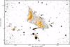 |
Fig. 1 WSRT 2273 MHz total intensity radio image. Contours are drawn at [1, 2, 4, 8]
× 3σ, with 3σ = 8 ×
10-5 Jy/beam and the color scale starts at the same
level. The beam size is |
4. Radio analysis and results
4.1. Radio images
4.1.1. WSRT image
In Fig. 1 we present the 2273 MHz total intensity
WSRT image of the central region of A 2256. The image has been produced with natural
weighting of the visibilities in the range [umin − umax ] = [ 260−21
035 λ]. The shortest spatial frequency sampled
umin determines the largest spatial
scale recovered by this observations  . The image has been corrected for the
primary beam attenuation that determines an increase of the noise in the edge of the
image. The high resolution (
. The image has been corrected for the
primary beam attenuation that determines an increase of the noise in the edge of the
image. The high resolution ( ) allowed us to analyze the
substructures of the diffuse relic emission in detail. The map shows several of the
well-known radio features present in the cluster (notation from Bridle et al. 1979; Rottgering et al.
1994): the radio relic emission (sources G and H), the head-tail sources A, B,
C and I, the complex source F (here resolved in the three components F1, F2 and F3), as
well as many other discrete sources, some of which labeled in this paper as I2, I3, K2,
G2, J2. The radio halo emission present in the center of the cluster around source D
(Clarke & Ensslin 2006) is completely
filtered out due to a combination of effects: its low surface brightness at this
frequency, combined with the lack of sampled short spacings in the WSRT observations,
that determines the loss of the very extended weak emission.
) allowed us to analyze the
substructures of the diffuse relic emission in detail. The map shows several of the
well-known radio features present in the cluster (notation from Bridle et al. 1979; Rottgering et al.
1994): the radio relic emission (sources G and H), the head-tail sources A, B,
C and I, the complex source F (here resolved in the three components F1, F2 and F3), as
well as many other discrete sources, some of which labeled in this paper as I2, I3, K2,
G2, J2. The radio halo emission present in the center of the cluster around source D
(Clarke & Ensslin 2006) is completely
filtered out due to a combination of effects: its low surface brightness at this
frequency, combined with the lack of sampled short spacings in the WSRT observations,
that determines the loss of the very extended weak emission.
The relic emission exhibits two regions of enhanced surface brightness: a well-defined
arc-like region (G region) in the northern part, and a less defined region (H region) in
the western part (see Fig. 1). The two regions are
connected by a bridge of lower brightness emission. At full resolution the entire relic
emission covers an area of about  . The size reported by Clarke & Ensslin (2006) at 1.4 GHz and at a
resolution of 52′′ × 45′′ is
. The size reported by Clarke & Ensslin (2006) at 1.4 GHz and at a
resolution of 52′′ × 45′′ is
 . Convolving our WSRT image to the same
resolution we obtain a similar angular size (not shown). Nevertheless, as we might be
anyway missing some of the flux on the most extended scales, we do not use this image
for the computation of the relic integrated spectrum.
. Convolving our WSRT image to the same
resolution we obtain a similar angular size (not shown). Nevertheless, as we might be
anyway missing some of the flux on the most extended scales, we do not use this image
for the computation of the relic integrated spectrum.
4.1.2. EFFELSBERG images
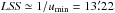
In Fig. 2 we show the 2640 MHz (left panel) and 4850 MHz (right panel) Effelsberg images of A 2256. In both images, the diffuse emission from the relic is mixed up with the emission from the more compact sources present in the field due to the low resolution of the observations. In the 2640 MHz image the relic emission is blended with the emission from the A+B+C complex and from source F. At 4850 MHz it is easier to separate the relic emission from the emission of the A+B complex, but still part of the tail of source C is inevitably superimposed on the western part of the relic. Moreover, Brentjens (2008) derived a spectrum α = 1.5 ± 0.2 for the radio halo between 351 and 1369 MHz. If there is no steepening in the spectrum of the halo, we expect a flux density of ~37 mJy at 2640 MHz and a flux density of ~15 mJy at 4850 MHz. Since a single dish is sensitive to all the emission in the field, its emission is smoothed with the other sources in our Effelsberg images if the halo spectrum keeps straight at these frequencies. Constraining the halo spectrum at high frequencies would require a dedicated careful analysis that is beyond the aims of this paper.
4.2. Spectral analysis
For the spectral analysis of the radio relic in A 2256 we combined our high-frequency observations with images obtained at other frequencies provided by the authors: the 351 MHz WSRT image (Brentjens 2008), the 1369 MHz VLA C and D configuration images7 (Clarke & Ensslin 2006) and the Effelsberg 10 450 MHz image (Thierbach 2000). We moreover got information on the flux densities in the LOFAR image at 63 MHz published by van Weeren et al. (2012) by the author. All the different images were calibrated according to the flux scale of Baars et al. (1977) or to its extension to lower frequencies (below 408 MHz; Perley & Taylor 1999)8. In this way we were able to cover the widest range of frequencies (63 MHz−10.45 GHz) used so far for the determination of the spectrum of a radio relic.
 |
Fig. 2 Effelsberg total intensity radio images. Left panel: Effelsberg
2640 MHz total intensity radio image in color scale and black contours drawn at [–1,
1, 2, 4, 8, 16] ×
3σ,
with 3σ = 4 ×
10-3 Jy/beam. The beam size is
|


We estimated the uncertainties σS on the flux density
measurements S with the following formula
 (4)where
-
 is the error due to the image noise,
with σ
being the image noise level (quoted in the image’s captions) and Nbeam the
number of beams covered by the source;
is the error due to the image noise,
with σ
being the image noise level (quoted in the image’s captions) and Nbeam the
number of beams covered by the source; -
σcal = Ecal × S is the error due to calibration uncertainties, determined in turn by two factors: the accuracy of the absolute flux density scale adopted (ϵscale) and the uncertainties related to the application of such scale to our data (the calibration method, ϵcal); being these two factors uncorrelated we used
 .
.
The spectral data provided by Baars et al. (1977) for the flux density calibrators have an absolute uncertainty of 5%. For the calibration of the Effelsberg images we performed four coverages of 3C 286 and three coverages of 3C 48 at 2640 MHz and four coverages of 3C 286 and three coverages of NGC 7027 at 4850 MHz. A Gaussian fit of the image of a calibrator provides its flux density in map unit. A comparison of this value with the known calibrator flux density allows us to calculate the factor to translate map unit in physical unit. The slightly different factors deriving from the different coverages of the calibrators were finally averaged, separately at the two frequencies. The standard deviation of these values (at the two frequencies) was used as the term ϵcal. For the WSRT data we used, instead, the dispersion of antenna gains. This translates into ϵcal values of 1.6% for the Effelsberg 11 cm data, of 1.2% for the Effelsberg 6 cm data and of 2% for the WSRT 13 cm data. Combining this with the uncertainties on the Baars et al. (1977) scale, we end up with Ecal(11 cm) = 5.3%, Ecal(6 cm) = 5.2% and Ecal(13 cm) = 5.4%. For the other images from the literature we assumed a similar value Ecal = 6%. It should be noted that the self-calibration process might affect the measured flux densities on interferometric images. The uncertainties are therefore possibly larger than estimated here.
Where not otherwise specified, we estimated the uncertainties σf on the quantities
f
calculated from measured quantities (e.g., spectral indices and extrapolated flux
densities of discrete sources) applying the standard error propagation formula. The
spectra of the total cluster, relic+sources, relic, G and H regions presented in the next
sections have been determined calculating the flux densities at different frequencies on
images convolved to the same lowest resolution available
( ) and using the same regions for the
integration. The errors associated to the spectral indices are the errors from the fits of
the data taking into account the uncertainties in the flux density measurements.
) and using the same regions for the
integration. The errors associated to the spectral indices are the errors from the fits of
the data taking into account the uncertainties in the flux density measurements.
All the spectra, including those of the discrete sources embedded in the relic emission, are plotted over the same fixed x-axis range (frequency range 40−14 000 MHz) for easy comparison.
4.2.1. Total cluster emission
We first considered the integrated radio flux density of the entire cluster (halo, relic and discrete sources combined) measuring the flux density in the circular region centered at J2000 position α = 17 03 45δ = + 78 43 00 with 10′ radius, as described by Brentjens (2008). The cluster radius was determined by Brentjens (2008) as the one at which the derivative of the integrated flux within the circle respect to the radius of the circle settles to a constant value. The measured flux densities at 351, 1369 (D configuration), 2640, 4850 and 10 450 MHz are summarized in Table 4. The total cluster radio emission between 351 and 10 450 MHz can be modeled by a single power law with spectral index α = 1.01 ± 0.02 (Fig. 10a).
Brentjens (2008) modeled the cluster flux density as the sum of two spectral components, one due to the halo and the other due to the relic and discrete sources combined. He showed that the second term becomes dominant at frequencies above 100 MHz. Being the radio relic the dominant contributor to the flux density at high frequency, its spectrum at the same frequencies cannot be flatter than the total cluster emission spectrum. This shows qualitatively that at high frequencies the relic spectrum does not keep the 0.85 slope observed at low frequency by van Weeren et al. (2012). In Sect. 4.2.3 we will quantify this steepening.
Properties of the radio sources embedded in the radio relic emission.
4.2.2. Discrete sources
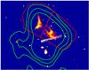 |
Fig. 3 Regions used for the spectra computation. The red region marks the region considered for the relic spectrum computation. The total region is further subdivided into regions G and H. In color scale the WSRT high-resolution image with the green contours from the 2640 MHz Effelsberg image overplotted. The white region mark the C source. |
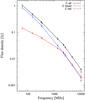 |
Fig. 4 Integrated radio spectrum of source C. Filled circles are measured flux densities while open circles are extrapolated flux densities. The black solid line is the spectrum of the entire source; the red dashed line is the source’s head spectrum; the blue dotted-dashed line is the spectrum of the tail. See text for more details. |
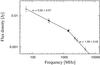 |
Fig. 5 Integrated radio spectrum of source K. Filled circles are measured flux densities while open circles are extrapolated flux densities. |
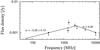 |
Fig. 6 Integrated radio spectrum of source J. Filled circles are measured flux densities while open circles are extrapolated flux densities. |
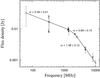 |
Fig. 7 Integrated radio spectrum of source I. Filled circles are measured flux densities while open circles are extrapolated flux densities. |
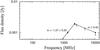 |
Fig. 8 Integrated radio spectrum of source I2. Filled circles are measured flux densities while open circles are extrapolated flux densities. |
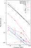 |
Fig. 9 Integrated radio spectra of the different components in the relic region shown in
Fig. 3. In black we show the flux densities
and spectra of the emission from the entire region (relic+sources). The dashed
( |
Figure 3 shows the area selected for measuring the radio relic flux densities. From the high-resolution image it is possible to see which are the discrete sources included in such area: the tail of source C Ctail, K, J, I, G2, K2, J2, I2 and I3. To estimate the flux density from the discrete sources that needs to be subtracted from the total emission, we produced two images at 1369 MHz (VLA C configuration) and 2273 MHz (WSRT) using the same uv-range (262−15 460 λ), pixel-size and restoring beam and we calculated the spectral index of the discrete sources embedded in the relic emission between these two frequencies. Moreover we measured the flux density at 10 450 MHz for the different components of source C and for the sources J and I2. Where available, we combined our data with data collected from the literature and we modeled the integrated spectra of the discrete sources over the frequency range 63−10 450 MHz. All the measured and extrapolated flux densities, as well as the spectral indices of the source C components with references are listed in Table 3. Details on the flux densities derivation are given in Appendix A. The spectra of the sources C, K, J, I and I2, for which more than two flux density measurements were available, are plotted individually in figures from 4 to 8 and all together in red in Fig. 9. For the sources K2, J2, I3 and G2 only our flux density measurements at 1369 and 2273 MHz were available and we simply assumed straight spectra. This assumption may lead to a slight over estimate of the flux densities at both low and high frequencies (as for standard radio source synchrotron spectra we expect a flattening at low frequencies and a steepening at high frequencies). On the other hand, they are weak sources and their flux densities are not crucial for the relic spectrum determination. Their spectra are plotted in blue in Fig. 9. This figure shows the spectra of the discrete sources included in the region selected, compared to the total flux density in the region (relic+sources). The main flux density contribution among the discrete sources in the relic area come from the tail of source C, especially at lower frequencies. The source appears noticeably narrow and long at high resolution, ~410″ in total in our 2273 MHz image (see Fig. 3). The published flux densities in the literature refer to the source as a whole. We modeled the source distinguishing between the head (long 76″) and the tail as we are interested only on the contribution from the latter. In Fig. 4 the spectrum over the range 63−10 450 MHz is plotted for the entire source, the head, and the tail. As common among head-tail sources, the head is flatter than the tail and the spectrum steepens at high frequency for both components. At lower frequencies, the tail contains almost all the emission of the sources. At high frequencies the electrons in the tail are older while the head is more clearly visible.
Sources J and I2 have an inverted-spectrum. Their spectra (plotted in Figs. 6 and 8) have a convex shape at GHz frequencies, typical of inverted-spectrum sources, and are likely young radio objects.
4.2.3. Radio relic spectrum
To avoid that resolution effects at different frequencies may alter the determination
of the relic integrated spectrum, we convolved all the images used for the flux
densities computation to the same resolution of  . At such low resolution, it is not
easy to identify the region where to measure the relic flux density. We adopted the
following strategy: we first computed the relic flux density from the 4850 MHz image at
full resolution, where it is easier to separate the relic emission from the complex A+B
emission. We then choose the relic region in the 4850 MHz image convolved to the
resolution of
. At such low resolution, it is not
easy to identify the region where to measure the relic flux density. We adopted the
following strategy: we first computed the relic flux density from the 4850 MHz image at
full resolution, where it is easier to separate the relic emission from the complex A+B
emission. We then choose the relic region in the 4850 MHz image convolved to the
resolution of  , matching the flux density measured
at full resolution at the same frequency. The selected area is shown in Fig. 3. The region is further divided into two regions of
enhanced radio brightness (regions G and H) discussed in the next section. As discussed
in the previous section, this region include the radio relic and sources
Ctail, K, J, I,
G2, K2, J2, I2 and I3.
, matching the flux density measured
at full resolution at the same frequency. The selected area is shown in Fig. 3. The region is further divided into two regions of
enhanced radio brightness (regions G and H) discussed in the next section. As discussed
in the previous section, this region include the radio relic and sources
Ctail, K, J, I,
G2, K2, J2, I2 and I3.
Total cluster flux densities.
We first considered the total emission from the region. Although the flux density
measurements of the relic+sources in the range 63−10 450 MHz can be fitted with a single
power law with  (Fig. 9), hints of a steepening at frequencies >1400 MHz are present. A separate
fit of the spectra between 63 and 1369 MHz and between 1369 and 10 450 MHz shows indeed
that these two frequency ranges are best represented by two different power laws, with
(Fig. 9), hints of a steepening at frequencies >1400 MHz are present. A separate
fit of the spectra between 63 and 1369 MHz and between 1369 and 10 450 MHz shows indeed
that these two frequency ranges are best represented by two different power laws, with
 and
and
 (Fig. 9). All the fits are plotted over the entire range 63−10 450 MHz to highlight differences.
Since the relic is the major contributor in the region both at low and high frequency,
this suggests that a steepening might be present in its spectrum as well. Moreover the
relic spectrum between 63 and 1369 MHz must be
(Fig. 9). All the fits are plotted over the entire range 63−10 450 MHz to highlight differences.
Since the relic is the major contributor in the region both at low and high frequency,
this suggests that a steepening might be present in its spectrum as well. Moreover the
relic spectrum between 63 and 1369 MHz must be  as it cannot be steeper than the
relic+sources spectrum. Similarly it must be
as it cannot be steeper than the
relic+sources spectrum. Similarly it must be  as it cannot be flatter than the
relic+sources spectrum. Indeed, after discrete sources subtraction we find that,
although the relic spectrum between 63 and 10 450 MHz is not inconsistent with a single
power law with
as it cannot be flatter than the
relic+sources spectrum. Indeed, after discrete sources subtraction we find that,
although the relic spectrum between 63 and 10 450 MHz is not inconsistent with a single
power law with  , it is best represented by two different
power laws, with
, it is best represented by two different
power laws, with  and
and
 (Fig. 10b). This is supported by a lower
values of the reduced χ2 in the case of the double power law
(
(Fig. 10b). This is supported by a lower
values of the reduced χ2 in the case of the double power law
( ) respect to the single power law
(
) respect to the single power law
( ). The measured relic flux densities
(before and after discrete sources subtraction) are summarized in Table 5. The flux densities measured at 63 MHz, 351 MHz and
1369 MHz are in agreement within the error bars with the already published flux
densities at the same frequencies. The low-frequency spectral index is in agreement with
what was found by van Weeren et al. (2012).
). The measured relic flux densities
(before and after discrete sources subtraction) are summarized in Table 5. The flux densities measured at 63 MHz, 351 MHz and
1369 MHz are in agreement within the error bars with the already published flux
densities at the same frequencies. The low-frequency spectral index is in agreement with
what was found by van Weeren et al. (2012).
Clarke & Ensslin (2006) report a relic mean spectral index between 1369 MHz and 1703 MHz of 1.2. However, this value has a big uncertainty (not quoted by author) since it is derived as the mean value from the spectral index image between two very close frequencies. We cannot therefore exclude it is in agreement with our value. Moreover, the very recent JVLA observations by Owen et al. (2014) reports for the relic an overall intensity weighted spectral index in the L-band of ~0.94, in agreement with our finding.
4.2.4. Regions G and H
Our high-resolution image shows that the relic can be divided into two separate parts:
regions G and H in Fig. 3. The cases of double
relics in the same cluster are getting more and more common since the first discovery of
two almost symmetric relics located on opposite sides in A3667. Since then, several
other double relics systems have been found (see Feretti et al. 2012). We have
investigated the possibility that the two different parts have different properties
fitting the spectra in the frequency range 351−10 450 MHz, separately. After discrete sources subtraction, the
flux densities of region G can be fitted with a single power law with a spectral index
of  (Fig. 10c). For homogeneity with the
radio relic analysis, we performed a separate fit of the spectra between 351 and 1369
MHz and between 1369 and 10 450 MHz. We find
(Fig. 10c). For homogeneity with the
radio relic analysis, we performed a separate fit of the spectra between 351 and 1369
MHz and between 1369 and 10 450 MHz. We find  and
and
 (Fig. 10c).
For the H region the flux densities can be modeled with a single power law with
spectral index  or with a double law with the same slope
as the G region at low frequency
or with a double law with the same slope
as the G region at low frequency  and a bit flatter spectra respect the G
region at high frequency
and a bit flatter spectra respect the G
region at high frequency  (Fig. 10d).
The measured flux densities before and after discrete sources subtraction are listed in Tables 6 and 7, while the spectra are plotted in Figs. 10c and 10d.
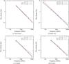 |
Fig. 10 Integrated radio spectra. The red dashed and blue dot-dashed lines are a double power-law fit to the data while the solid black line is the single power-law fit. In panel b) the green crosses are the upper limits to the radio relic flux taking into account the SZ effect. See text for more details. |
Radio relic flux densities.
Region G flux densities.
Region H flux densities.
Observed synchrotron spectral indices of the different components.
5. X-ray analysis and results
5.1. ICM temperature
In the course of a merger, a significant portion of the energy involved is dissipated by
shocks and turbulence leading eventually to the heating of the ICM gas. As mentioned in
the Introduction, in the test particle regime of DSA theory the shock structure is
determined by the canonical shock jump conditions (Rankine-Hugoniot). Applying these
conditions, assuming the ratio of specific heats as 5/3, the expected ratio between the
postshock and preshock temperatures, respectively T2 and
T1, is related to the shock Mach number
through the following relation: 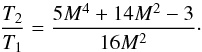 (5)We extracted the ICM temperature in different
regions across the radio relic corresponding to the rectangular areas shown in Fig. 11. The observed spectra were assumed to consist of thin
thermal plasma emission from the ICM, plus the total background contamination described in
Sect. 3. The emission from the ICM was modeled with
an additional absorbed thermal component in the total model (ICM+background). For the
Suzaku analysis, to generate the auxiliary response files (ARF), we
used an image constructed using a β-model (β = 0.816, rc =
5.64′ from Markevitch & Vikhlinin
1997) as input for the xissimarfgen. For XMM-Newton data,
we fitted the spectra in the 0.5−8 keV energy range, excluding the 1.4−1.6 keV band due to the strong
contamination from the Al line in all three detectors. Because of the low number of counts
in the XMM-Newton spectra of region r1, r2 and r3, we kept the
metallicity values in the fit frozen to the value obtained with the Suzaku
analysis, which are better constrained9.
Temperatures and normalizations of the thermal components were allowed to vary in the fit.
(5)We extracted the ICM temperature in different
regions across the radio relic corresponding to the rectangular areas shown in Fig. 11. The observed spectra were assumed to consist of thin
thermal plasma emission from the ICM, plus the total background contamination described in
Sect. 3. The emission from the ICM was modeled with
an additional absorbed thermal component in the total model (ICM+background). For the
Suzaku analysis, to generate the auxiliary response files (ARF), we
used an image constructed using a β-model (β = 0.816, rc =
5.64′ from Markevitch & Vikhlinin
1997) as input for the xissimarfgen. For XMM-Newton data,
we fitted the spectra in the 0.5−8 keV energy range, excluding the 1.4−1.6 keV band due to the strong
contamination from the Al line in all three detectors. Because of the low number of counts
in the XMM-Newton spectra of region r1, r2 and r3, we kept the
metallicity values in the fit frozen to the value obtained with the Suzaku
analysis, which are better constrained9.
Temperatures and normalizations of the thermal components were allowed to vary in the fit.
We observe a temperature drop across the G region of the radio relic, with the
temperature jumping from 8.45 keV in the region r2 (on the relic) to
4.95
keV in the region r2 (on the relic) to
4.95 keV in the region r3 (outside the outer
edge of the relic). XMM-Newton measurements in the same regions provide
consistent temperatures although with bigger errors. This is in agreement with Sun et al. (2002) that found a hot region
(~9 KeV) in positional
coincidence with the G lobe of the radio relic. Radio relics are usually associated to
outgoing merger shocks that travels from the core of a merging event outwardly towards the
periphery of the clusters. If we apply such scenario to A 2256, connecting the radio relic
emission to a shock front propagating outwardly in the north-western direction across the
G region of the radio relic, we can consider r2 as the post-shock region and r3 as the
preshock region. In this case we have a temperature ratio T2/T1
= 1.7. It is important to notice that this estimate is impacted by the
angle of the shock front to the line of sight. If the shock is not in the plane of the
sky, as it is likely the case for A 2256, projected mixing of shocked hot gas with cool
gas will reduce the apparent temperature of the shocked gas and increase the apparent
temperature of the cool gas, basically dropping the temperature ratio.
keV in the region r3 (outside the outer
edge of the relic). XMM-Newton measurements in the same regions provide
consistent temperatures although with bigger errors. This is in agreement with Sun et al. (2002) that found a hot region
(~9 KeV) in positional
coincidence with the G lobe of the radio relic. Radio relics are usually associated to
outgoing merger shocks that travels from the core of a merging event outwardly towards the
periphery of the clusters. If we apply such scenario to A 2256, connecting the radio relic
emission to a shock front propagating outwardly in the north-western direction across the
G region of the radio relic, we can consider r2 as the post-shock region and r3 as the
preshock region. In this case we have a temperature ratio T2/T1
= 1.7. It is important to notice that this estimate is impacted by the
angle of the shock front to the line of sight. If the shock is not in the plane of the
sky, as it is likely the case for A 2256, projected mixing of shocked hot gas with cool
gas will reduce the apparent temperature of the shocked gas and increase the apparent
temperature of the cool gas, basically dropping the temperature ratio.
Regions r5 and r4, respectively on the H region of the relic and outside the outer edge,
show almost equal temperatures  and
and
 in the XMM-Newton images,
although with big uncertainties. Unfortunately, region r4 is out of Suzaku
field-of-view and cannot be checked. This is anyway in agreement with previous
studies conducted by Sun et al. (2002) and Bourdin & Mazzotta (2008) that showed that this
region is cold due to the presence of a cool subcluster at an early stage merging with the
main cluster, approaching from somewhere west. Projection effects, affecting in particular
region r5, can thus be responsible for the non detection of a temperature jump across the
H region of the relic.
in the XMM-Newton images,
although with big uncertainties. Unfortunately, region r4 is out of Suzaku
field-of-view and cannot be checked. This is anyway in agreement with previous
studies conducted by Sun et al. (2002) and Bourdin & Mazzotta (2008) that showed that this
region is cold due to the presence of a cool subcluster at an early stage merging with the
main cluster, approaching from somewhere west. Projection effects, affecting in particular
region r5, can thus be responsible for the non detection of a temperature jump across the
H region of the relic.
The measured temperatures in the different regions are summarized in Table 9 for both Suzaku and XMM-Newton data.
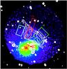 |
Fig. 11 Regions used for the ICM temperature extraction. Colors show the XMM-Newton X-ray image, while the contours show the radio emission at a lower resolution respect to Fig. 1. |
CM temperatures kT(keV).
6. Is the Sunyaev-Zeldovich effect important?
The thermal Sunyaev-Zeldovich (SZ) effect (Sunyaev & Zeldovich 1970) consists in the inverse Compton scattering to higher energies of the photons of the Cosmic Microwave Background (CMB) that interact with the hot electrons in the ICM of galaxy clusters. The effect depends on the pressure produced by the plasma along the line of sight and is parametrized through the Comptonisation parameter y (see Carlstrom et al. 2002, for a review). The SZ effect produces a modification of the CMB blackbody spectrum, creating a negative flux bowl on the scale of the cluster, at GHz frequencies. This might lead to two sources of errors in our flux densities measurements at high frequencies. The first derives from a wrong setting of the zero-level in the single dish images. The zero-level in single dish observations is usually set assuming the absence of sources at the map edges, setting the intensity level to zero there, and interpolating linearly between the two opposite edges of the map. If the SZ decrement is important in the regions where zero flux was assumed (determining a negative flux in those areas), this results in a wrong setting of the zero-level of the entire map. This lead to a lower estimation of the flux densities integrated over any region in the map. In addition to this, there is the SZ decrement specific to the area used to compute the relic flux densities.
We used the integrated Comptonisation parameter YSZ as measured by Planck (Planck Collaboration XI 2011) and the universal pressure profile shape as derived by Arnaud et al. (2010), to derive the predicted pressure and Comptonisation parameter profiles for A 2256 (see Planck Collaboration Int. IV 2013). We used the derived y parameter radial profile to estimate the importance of the SZ decrement in different regions at the edges of the original Effelsberg 10 450 MHz image, to check the zero-level setting. Integrating on areas free of sources at the map edges with angular diameter of 4′, we find values of −0.1/−0.3 mJy for the CMB flux decrement. We conclude that the effect of the SZ decrement on the zero-level setting of the 10 450 MHz image is negligible. As the SZ effect increase increasing the frequency, we conclude that it does not affect the zero-level setting of the 2640 and 4850 MHz Effelsberg images.
Estimating the second effect is more complicated, especially if we believe that the relic in A 2256 is powered by a shock. In case of a shock, in fact, a sharp increase of the pressure at the shock front is expected, causing a local increase of the SZ decrement. An exact estimate of the amount of the effect requires a detailed knowledge of the shock geometry and orientation and of the pressure changes across the relic width. We estimate here an upper limit for the SZ effect on our high-frequencies flux estimates. The radio relic fluxes have been calculated in an approximatively rectangular area of ~18′ × 9′, whose major axis is located at a projected distance of ~7.2′ (~500 kpc) from the cluster X-ray main peak. If we assume that we observe the shock in the plane of the sky, we can consider a physical distance of the relic from the cluster center of ~500 kpc. This is a lower limit to the real distance relic-cluster center and maximize the SZ effect, that is higher in the denser central regions. We can derive a qualitative estimation of the possible shock pressure jump from the observed ICM temperature ratio across the relic. Inverting Eq. (5) we obtain a Mach number ~1.7. As discussed, this number can have been reduced by projection effects. We assume for the calculations a Mach number M = 2. Applying the Rankine-Hugoniot jump conditions, the ratio between the postshock P2 and preshock P1 pressures, given the Mach number M, is P2/P1 ~ 4. We estimated the SZ flux decrement in the area used for the radio relic flux measurements using Eq. (3) from Carlstrom et al. (2002) and assuming a value yPOST = 4yPRE (where yPRE was extracted from the y-profile at a corresponding distance of 7.2′) constant over all the area. This assumptions bring to an over estimation of the SZ effect because the real width of the relic is expected to be much lower than the projected one, and the increased pressure is expected to decrease again moving away from the shock front in the downstream region. With these assumptions, we obtain SZ flux decrements of ~–20 mJy, ~–4.3 mJy, ~–0.3 mJy respectively at 10 450 MHz, 4850 MHz and 2640 MHz. We stress that this numbers are upper limits for the SZ decrement. Assuming, for example, the physical distance of ~700 Kpc from the cluster center deduced by Ensslin et al. (1998) based on polarization properties, the effect at 10 450 MHz reduces to ~–11 mJy.
We plotted in Fig. 10b (green crosses) the upper limits of the relic flux at 4850 and 10 450 MHz, derived adding the upper limit SZ flux decrements (in absolute value) to the measured fluxes. The effect on the integrated radio spectrum is to make it even flatter.
7. Discussion
Independent of the acceleration mechanism, we can infer the range of energies (in terms of
the Lorentz factor γe) of the emitting electrons in the relic
region from the integrated spectrum via (Kang et al.
2012): 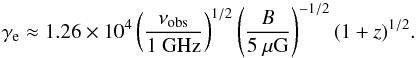 (6)The relic in A 2256 has been observed from very
low frequencies (~20 MHz
with LOFAR, van Weeren et al. 2012, flux densities
not published) up to very high frequencies (~10 GHz with Effelsberg). This implies, via Eq. (6), that the emitting electrons have energies
between, at least, γe,min ~ 2 × 10³−4 ×
103 and γe,max ~ 4 × 10⁴−9 ×
104. For both γe,min and γe,max, the two
values refer to assumed magnetic fields B = 5−1 μG, respectively. The energy
losses of low-energy electrons can be dominated by Coulomb interactions with the plasma,
causing a low-frequency flattening of the integrated spectrum, in the case that the density
in the relic region is rather high and the strength of the magnetic field is low (Sarazin 1999). The double power law found for the relic
in A2256 can be looked at as due to a low-frequency flattening other than a high-frequency
steepening. However, assuming an electron density of 10-3 cm-3 as estimated by Markevitch & Vikhlinin (1997) at the relic position
in A2256, and a typical value of 1 μG for the magnetic field, we calculated (from Eqs.
(7) and (9) in Sarazin 1999) that Coulomb losses do
not dominate over synchrotron losses even for the lowest energy electrons in our range
(γ ~
103). The radiative lifetime for the less energetic electrons
is trad(γe,min) ~
0.32−0.43 Gyr (for B = 5−1 μG respectively) and
trad(γe,max) ~
0.016−0.019 Gyr for the more energetic ones. Probably, whatever it is the
acceleration mechanism, it is still at work since the particles emitting at 10 GHz lose
rapidly their energy and the relic would become invisible at this frequency without a
constant supply of new particles, soon after the end of the acceleration. It is then
reasonable to consider, in case of DSA, a continuous injection model with radiative losses
dominated by IC and synchrotron emission to discuss the integrated spectrum of the radio
relic in A2256, as it is common in the literature.
(6)The relic in A 2256 has been observed from very
low frequencies (~20 MHz
with LOFAR, van Weeren et al. 2012, flux densities
not published) up to very high frequencies (~10 GHz with Effelsberg). This implies, via Eq. (6), that the emitting electrons have energies
between, at least, γe,min ~ 2 × 10³−4 ×
103 and γe,max ~ 4 × 10⁴−9 ×
104. For both γe,min and γe,max, the two
values refer to assumed magnetic fields B = 5−1 μG, respectively. The energy
losses of low-energy electrons can be dominated by Coulomb interactions with the plasma,
causing a low-frequency flattening of the integrated spectrum, in the case that the density
in the relic region is rather high and the strength of the magnetic field is low (Sarazin 1999). The double power law found for the relic
in A2256 can be looked at as due to a low-frequency flattening other than a high-frequency
steepening. However, assuming an electron density of 10-3 cm-3 as estimated by Markevitch & Vikhlinin (1997) at the relic position
in A2256, and a typical value of 1 μG for the magnetic field, we calculated (from Eqs.
(7) and (9) in Sarazin 1999) that Coulomb losses do
not dominate over synchrotron losses even for the lowest energy electrons in our range
(γ ~
103). The radiative lifetime for the less energetic electrons
is trad(γe,min) ~
0.32−0.43 Gyr (for B = 5−1 μG respectively) and
trad(γe,max) ~
0.016−0.019 Gyr for the more energetic ones. Probably, whatever it is the
acceleration mechanism, it is still at work since the particles emitting at 10 GHz lose
rapidly their energy and the relic would become invisible at this frequency without a
constant supply of new particles, soon after the end of the acceleration. It is then
reasonable to consider, in case of DSA, a continuous injection model with radiative losses
dominated by IC and synchrotron emission to discuss the integrated spectrum of the radio
relic in A2256, as it is common in the literature.
We have formulated five different possible scenarios to explain the properties of the relic, and we will discuss here the pros and cons for each of them.
7.1. Non-stationary DSA
Together, the regions G and H of the relic in A 2256 reach a length of ~1 Mpc. To date the most plausible scenario to explain such giant radio relics invoke diffusive shock acceleration (DSA) during cluster mergers. In this scenario, electrons are accelerated to an injection power-law spectrum at the shock location, and lose energy due to synchrotron and IC processes advecting downstream, causing a local steepening of the spectrum, the entity of which changes with the distance to the shock front. The continuous injection model is used to describe the situation in which these different regions are not spatially resolved and their contribution is mixed up. Assuming that the shock is continuously accelerating particles following the same power law for a time exceeding the electrons cooling time, we expect a volume-integrated spectrum that is a single straight power law with spectral index αobs = αinj + 0.5 (stationarity for the spectrum). As shown in Sect. 4.2.3, the relic in A 2256 shows, instead, a peculiar broken power law. At low frequencies (between 63 and 1369 MHz), we confirm the spectral index α ~ 0.85 previously found by van Weeren et al. (2012). This spectrum is too flat to be considered the stationary spectrum as it would imply an injection spectral index ~ 0.35, flatter than the flattest allowed by test-particle DSA theory (see Introduction). One solution is that, at low frequencies, we observe the injection synchrotron spectrum since a stationary spectrum is only attained if the time for energy losses is shorter than the age of the shock at all energies. Kang (2011) shows that the downstream integrated electron spectrum at a quasi-parallel shock is a broken power law which steepens from E− δinj to E− (δinj + 1) above E>Ebr(t), with an exponential cutoff at energies higher than Eeq. Eeq is the maximum electron energy injected, reached when the equilibrium between energy gains and losses is achieved and reflects the strength of the shock. Ebr describes more properly the electron aging and can be used to estimate the shock age. As a consequence the volume-integrated synchrotron spectrum has a spectral break and an high-frequency cut-off described by:
![$$ S(\nu) \propto \begin{cases} \nu ^{- \alpha_{\rm inj}} & \text{at } \nu <\nu_{\rm br} (t) \\[2mm] \nu ^{- (\alpha_{\rm inj}+0.5)} & \text{at } \nu_{\rm br} (t) <\nu <\nu_{\rm eq}\\[2mm] \exp(-\nu/\nu_{\rm eq}) & \text{at } \nu > \nu_{\rm eq}. \end{cases} $$](/articles/aa/full_html/2015/03/aa23972-14/aa23972-14-eq175.png) If we assume that the shock started to
accelerate particles recently, we would be able to catch the break frequency and the
transition from αinj to αobs still in
the observable frequency range (non-stationarity for the spectrum), as it happens for
young radio galaxies (e.g., Murgia et al. 1999).
Assuming a νbr
~ 1.4 GHz (in correspondence of which we observe the moderate
steepening) would imply a relic age of trad(γe,1.4 GHz) ~
0.04−0.05 Gyr. An injection spectral index ~0.85 would be also in agreement with
what reported by Clarke et al. (2011). They observe
a spectral index of 0.85 at the outer edge of the relic, steepening moving across the
source towards the inner edge. This is in agreement with a scenario where the relic is
produced by a shock that is moving outwardly and is now located at the outer edge of the
relic where it is accelerating particle according to an injection spectrum with
αinj =
0.85. However, Owen et al.
(2014) recently found that the simple gradient from north to south in spectral
index does not dominate the relic structure when observed in more detail. Moreover, the
spectral index of the integrated synchrotron emission above the break frequency should be
in this case αobs
~ 1.35, while we observe a flatter spectrum with slope
~1. However, the
spectral curvature of the continuous injection model is gradual and might occur over a
broader range of frequencies than sampled here. This would place the break frequencies at
frequencies even higher than 1.4 GHz, further reducing the radiative lifetime of the
relic. This would make the radio relic in A2256 a very young radio relic.
If we assume that the shock started to
accelerate particles recently, we would be able to catch the break frequency and the
transition from αinj to αobs still in
the observable frequency range (non-stationarity for the spectrum), as it happens for
young radio galaxies (e.g., Murgia et al. 1999).
Assuming a νbr
~ 1.4 GHz (in correspondence of which we observe the moderate
steepening) would imply a relic age of trad(γe,1.4 GHz) ~
0.04−0.05 Gyr. An injection spectral index ~0.85 would be also in agreement with
what reported by Clarke et al. (2011). They observe
a spectral index of 0.85 at the outer edge of the relic, steepening moving across the
source towards the inner edge. This is in agreement with a scenario where the relic is
produced by a shock that is moving outwardly and is now located at the outer edge of the
relic where it is accelerating particle according to an injection spectrum with
αinj =
0.85. However, Owen et al.
(2014) recently found that the simple gradient from north to south in spectral
index does not dominate the relic structure when observed in more detail. Moreover, the
spectral index of the integrated synchrotron emission above the break frequency should be
in this case αobs
~ 1.35, while we observe a flatter spectrum with slope
~1. However, the
spectral curvature of the continuous injection model is gradual and might occur over a
broader range of frequencies than sampled here. This would place the break frequencies at
frequencies even higher than 1.4 GHz, further reducing the radiative lifetime of the
relic. This would make the radio relic in A2256 a very young radio relic.
One disadvantage of integrated spectra is that the spectra of different source components are mixed up. The radiative ages derived from these spectra do not necessarily represent the source ages, but rather the radiative ages of the dominant source components. For radio galaxies, for example, only when the lobes (which have accumulated the electrons produced over the source lifetime) dominate the source spectrum, the radiative age derived from the νbr is likely representative of the age of the entire source. If, instead, the spectrum is dominated by the jets or hot spots, the radiative age likely represents the permanence time of the electrons in that component and is expected to be -perhaps much- less than the source age (Murgia et al. 1999). Something similar might hold for the radio relic in A2256 if its synchrotron emission is dominated by the shock region. This might happen because the magnetic field is expected to be stronger at the shock location due to shock compression (Lucek & Bell 2000). The continuous injection model assumes, instead, a constant magnetic field over all the source, and might not be optimal to describe the integrated spectra of radio relics. In general, if the latter are dominated by the emission from the regions closer to the shock front, they are biased to flatter values. As a consequence, the shock Mach numbers derived from radio observable through Eqs. (1)−(3) are biased to higher values. This would also account for the discrepancies between the values of the Mach number derived from radio observations vs values derived from X-ray observations claimed in some case (e.g., in the cluster ZwCl 2341.1+0000, Ogrean et al. 2014).
The observed radio spectrum of the relic in A 2256 may be reconciled with shock acceleration even invoking a more complex situation in which the electrons emitting in the relic region belong to different populations with different acceleration history. This might be due to a modification of the shock properties while propagating in the ICM (non-stationarity for the shock) and a consequent modification of the electron injection power law. Indeed, shocks developing in the core of a merging event will typically strengthen moderately as they propagate into lower density and low-temperature regions outside the cluster cores (Brunetti & Jones 2014). This results in a flattening of the injection power law as the shock propagates.
A combination of the two effects might take place in the A2256 relic, with consequences on the integrated spectrum that are difficult to quantify. They could be responsible for the flat behavior of its integrated spectrum.
7.2. CRe modified DSA
The relic spectrum can be fitted also with a single power law between 63 MHz and 10 450
MHz with a spectral index  . In this case the relic in A2256 would be
the one with the flattest integrated spectrum known so far, according to the collection in
Table 4 in Feretti et al. (2012). The spectral
index would be even flatter if the SZ decrement approaches our upper limits estimate. It
would be quite unlikely that we are observing the injection spectrum because this would
imply that νbr>
10 GHz that is equivalent to say that the relic brightened more
recently than 0.016−0.019 Gyr.
So, if what we observe is the stationary spectrum, it would imply an injection spectral
index ~ 0.42, flatter
than the flattest allowed by test particle DSA. Such a flat radio spectrum should be
produced by a relatively strong shock, even though predictions on the Mach number are not
possible inside the test-particle approximation of DSA. However, we observe a low
temperature ratio of 1.7. Although projection effects might have reduced this value, we
speculatively consider unlikely that they could have hidden a strong shock as the one
required. However, the X-ray data examined in this paper do not allow us to firmly rule
out the presence of a shock front with Mach number typical for relics. Accurate profiles
of the ICM surface brightness and temperature from X-ray observations, as well as pressure
profiles from deep pointed SZ observations are needed to finally establish the presence of
a shock front in the location of the radio relic in A 2256.
. In this case the relic in A2256 would be
the one with the flattest integrated spectrum known so far, according to the collection in
Table 4 in Feretti et al. (2012). The spectral
index would be even flatter if the SZ decrement approaches our upper limits estimate. It
would be quite unlikely that we are observing the injection spectrum because this would
imply that νbr>
10 GHz that is equivalent to say that the relic brightened more
recently than 0.016−0.019 Gyr.
So, if what we observe is the stationary spectrum, it would imply an injection spectral
index ~ 0.42, flatter
than the flattest allowed by test particle DSA. Such a flat radio spectrum should be
produced by a relatively strong shock, even though predictions on the Mach number are not
possible inside the test-particle approximation of DSA. However, we observe a low
temperature ratio of 1.7. Although projection effects might have reduced this value, we
speculatively consider unlikely that they could have hidden a strong shock as the one
required. However, the X-ray data examined in this paper do not allow us to firmly rule
out the presence of a shock front with Mach number typical for relics. Accurate profiles
of the ICM surface brightness and temperature from X-ray observations, as well as pressure
profiles from deep pointed SZ observations are needed to finally establish the presence of
a shock front in the location of the radio relic in A 2256.
A solution is to take into account the shock modification induced by the dynamical reaction of the accelerated particles. The condition on the flattest possible injection index is due to the test-particle approach to DSA. In CR modified shocks, the compression ratio can be higher and the injection synchrotron spectra can be flatter than 0.5 (e.g., Blasi 2010).
7.3. DSA of pre-accelerated CRe
Kang & Ryu (2011) and Kang et al. (2012) argue that the existence of pre-accelerated CRs electrons might alleviate the problem of inefficient injection at weak shocks. They have suggested that the hot ICM first goes through a series of accretion shocks of high Mach numbers before getting subjected to weaker cluster merger shock, and that hence the ICM should contain some pre-existing CR population. Moreover, pre-existing non thermal particles might have been produced via turbulent re-acceleration (Brunetti & Lazarian 2007, 2011) or through p − p collisions of CR protons with thermal protons of the ICM (Miniati et al. 2001). This pre-existing CR population may contain many different electron populations and may be described by a cumulative power law f ∝ E− δpre. They show that if the spectrum of the pre-existing population is steeper than the spectrum that could be produced by the shock (δpre>δinj), then the re-accelerated CR spectrum gets flattened to E− δinj by DSA. In the opposite case (δpre<δinj), the re-accelerated CR spectrum is simply amplified by the factor of δinj/ (δinj − δpre) and retains the same slope as the slope of pre-existing CRs (Kang & Ryu 2011; Kang et al. 2012). Applying this to the radio relic in A 2256, we have to assume that the spectrum we observe has the same spectral slope as the one of the pre-existing population. In this case the shock we observe would be responsible only for the amplification of the particle spectrum. However, it is difficult to explain how the radio spectrum has kept such flat slope over a wide range of frequencies in spite of electron energy losses.
7.4. Adiabatic compression
The relic in A 2256 appears to be very filamentary. Enßlin & Brüggen (2002) presented detailed three-dimensional simulations of the passage of radio plasma cocoons filled with turbulent magnetic field through shock waves. They showed that, on contact with the shock wave, the radio cocoons are first compressed and finally torn into filamentary structures. Moreover, van Weeren et al. (2012) proposed a viewing angle of about 30° from edge-on and a a true distance of ~0.5 Mpc from the cluster center for the radio relic. Both these two characteristics favor of a scenario where the relic is the result of re-energization of fossil plasma by adiabatic compression. On the other hand, the large size of the relic and the flat spectrum at high frequency make this scenario unlikely.
7.5. Independent relics
Finally, regions G and H might be another example of two independent relics, for example two radio Phoenices produced by the same shock or by different shocks front. We have checked for different properties of the two regions calculating their individual radio-integrated spectra. Although the integrated spectrum of region G appears slightly steeper than that of region H, the two are consistently similar within the error bars and too flat to be reconciled with the observed ICM temperature ratio. The absence of a pronounced steepening in the individual spectra also rules out the double phoenics origin.
The above discussion leads to the conclusion that the radio relic in A2256 is a very special and complex case, which requires special conditions to be interpreted in the framework of DSA. Alternative models, e.g., magnetic reconnection, might be worth considering in this case, as suggested by Owen et al. (2014).
We presented in the introduction the radio relic in CIZA J2242.8+5301 as a textbook example of giant radio relic where the spectral predictions of the test-particle DSA model are nicely satisfied. Actually, it has been argued that this holds only at frequencies below 2.3 GHz, where the integrated spectrum and the spatial distribution of spectral indeces match the predictions from the test-particle DSA continuous injection model (Stroe et al. 2013). However, recent observations of the relic at 16 GHz (Stroe et al. 2014), shows a high-frequency steepening, with the flux density at this frequency lying 12σ below the extrapolation of the low-frequency single power-law spectrum. They argue that this discrepancy can be due to different factors, e.g., an injection spectrum that is not a power law, a gradient of density and/or temperature across the source, a non-homogeneity of the magnetic field. We suggest that another explanation could be that the observed steepening is the expected cut-off above Eeq. Due to the lack of flux density measurements between 2.3 and 16 GHz, the gradualness of the steepening can not be established and a firm comparison with the model’s expectation is not easy. Another possibility is that the low flux density is due to SZ decrement, that can be important over the large area covered by the radio relic in CIZA J2242.8+5301. Nevertheless, Stroe et al. (2014) conclude that at the moment no relic formation mechanisms can readily explain the high-frequency steepening and new theoretical models must be developed.
8. Conclusions
We presented new high-frequency observations of A 2256 performed at 2273 MHz with the WSRT and at 2640 and 4850 MHz with the Effelsberg 100 m Telescope. The main points of this study can be summarized as follows.
-
1.
The high resolution of the WSRT observations highlighted that the relic can be divided into two regions of enhanced surface brightness (regions G and H) connected by a filamentary bridge of lower brightness emission.
-
2.
Combining our new observations with images available at other frequencies, we constrained the radio-integrated spectrum of the radio relic in A 2256 over the widest sampled frequency range collected so far for this kind of object (63−10 450 MHz). We find that the relic keeps an unusual flat behavior up to high frequencies. We find that, although the relic spectrum between 63 and 10 450 MHz is not inconsistent with a single power law with
, a separate fit of the spectra between
63 and 1369 MHz and between 1369 and 10 450 MHz shows that these two frequency ranges
are best represented by two different power laws, with
and
. This broken power law would require
special conditions to be explained in terms of test-particle DSA, e.g., the
non-stationarity of the spectrum and/or the non-stationarity of the shock. On the
other hand, the single power law would make of this relic the one with the flattest
integrated spectrum known so far, even flatter than what is allowed in the
test-particle approach to DSA. -
3.
We investigated the possibility that the G and H regions have different properties in the frequency range 351−10 450 MHz. We find that the singular spectra of regions G and H show a similar flat trend with respect to the total relic with
and
. -
4.
We used Suzaku and XMM-Newton X-ray observations to measure the ICM temperature in the regions across the radio relic emission. We find a temperature ratio T2/T1 ~ 1.7 across the G region of the radio relic. Although projection effects might have reduced this value, we consider it unlikely that they could have hidden a strong shock such as the one required by the flat behavior of the integrated spectrum of the entire relic, as well as of the regions G and H separately. However, the X-ray data examined in this paper do not allow us to firmly rule out the presence of a shock front with the Mach number typical for relics. No temperature jumps are observed across the H region of the relic. This might be due to the projection in this area of a colder subcluster approaching the main cluster from the west.
-
5.
The absence of a pronounced steepening in the integrated radio spectrum of the total relic, as well as of the regions G and H separately, rules out a phoenices origin for the relic(s).
We conclude that the case of A2256 shows that the simple shock model with assumptions of continuous stationary injection, constant magnetic field across the relic regions, and stationarity of the shock properties is insufficient when the radio spectra are known over a broader range of frequencies. The complexity of current models invoking shock acceleration must, therefore, be increased. Alternative models might be worth considering in some cases.
Online material
Appendix A: Derivation of the flux densities of discrete sources
Here we report the details of the derivation of the discrete sources flux densities. All the values are listed in Table 3. The sources position in brackets are expressed in the J2000 coordinate system.
Source C tail (17 03 28, +78 39 57)
The peak of the emission of source C coincides with an optical galaxy with magnitude
15.3 (Bridle et al. 1979). The head-tail
morphology for source C was first suggested by Bridle
& Fomalont (1976). We modeled the source distinguishing between the head
(long 75 6)
and the tail as we are interested only on the contribution from the latter. At the
highest frequency (10 450 MHz) the head of the source is still clearly visible, while
it’s difficult to establish if the flux in the tail region is from the tail or from the
underlying relic. The measured fluxes are S(head)10 450 = 2.1 ±
0.6 mJy and S(tail)10 450 = 1.9 ±
0.7 mJy and consequently S(all)10 450 = 4.0 ±
0.0; the last two can be considered as upper limits. Combining this
values with the fluxes we measured at 2273 MHz (S(all)2273 =
33.7 ± 1.8 mJy; S(head)2273 = 17.3 ±
0.9 mJy; S(tail)2273 = 16.4 ±
0.9 mJy), we obtain spectral indeces
6)
and the tail as we are interested only on the contribution from the latter. At the
highest frequency (10 450 MHz) the head of the source is still clearly visible, while
it’s difficult to establish if the flux in the tail region is from the tail or from the
underlying relic. The measured fluxes are S(head)10 450 = 2.1 ±
0.6 mJy and S(tail)10 450 = 1.9 ±
0.7 mJy and consequently S(all)10 450 = 4.0 ±
0.0; the last two can be considered as upper limits. Combining this
values with the fluxes we measured at 2273 MHz (S(all)2273 =
33.7 ± 1.8 mJy; S(head)2273 = 17.3 ±
0.9 mJy; S(tail)2273 = 16.4 ±
0.9 mJy), we obtain spectral indeces
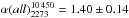 ,
, 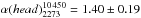 and
and
 . We used these values of the spectral
indeces to extrapolate the fluxes of the components at 2640 and 4850 MHz. Lin et al. (2009) report a measured flux for the
source C (referred to in the paper as 1706+787) of 5.06 ± 0.60 mJy at 4.9 GHz, classifying
the source as a point source. Due to the wrong classification, we believe that their
observations resolve out the tail of the source and the reported flux refers to the
source head only. Indeed, their reported flux is in agreement with the flux that we
extrapolated for the head of the source (S(head)4850 = 6.0 ±
0.9 mJy).
. We used these values of the spectral
indeces to extrapolate the fluxes of the components at 2640 and 4850 MHz. Lin et al. (2009) report a measured flux for the
source C (referred to in the paper as 1706+787) of 5.06 ± 0.60 mJy at 4.9 GHz, classifying
the source as a point source. Due to the wrong classification, we believe that their
observations resolve out the tail of the source and the reported flux refers to the
source head only. Indeed, their reported flux is in agreement with the flux that we
extrapolated for the head of the source (S(head)4850 = 6.0 ±
0.9 mJy).
Rottgering et al. (1994) report a flux for the
entire source at 327 MHz of 246 ± 20 mJy; combining this with our measurements at 1369 MHz
(S(all)1369 = 56.5 ±
3.4) we find that the spectral index for the entire source keeps the
same slope as in the range 1369−2273 MHz,  . To separate the emission between the
head and the tail we used the spectral index profile along the tail of the source C
between 327 and 1447 MHz published by Rottgering et al.
(1994, Fig. 7 right side). From the plot we deduced that the averaged spectral
index of the head (selecting the range 0−
~ 75′′ in the x axes) is
. To separate the emission between the
head and the tail we used the spectral index profile along the tail of the source C
between 327 and 1447 MHz published by Rottgering et al.
(1994, Fig. 7 right side). From the plot we deduced that the averaged spectral
index of the head (selecting the range 0−
~ 75′′ in the x axes) is
 . From this we got a flux at 327 MHz for
the head of 63.4 mJy and consequently a flux for the tail of S(tail)327 =
246.0−63.4 = 182.6 and a spectral index
. From this we got a flux at 327 MHz for
the head of 63.4 mJy and consequently a flux for the tail of S(tail)327 =
246.0−63.4 = 182.6 and a spectral index
 . We used this spectral index to
calculate the fluxes at 351 MHz.
. We used this spectral index to
calculate the fluxes at 351 MHz.
At 153 MHz van Weeren et al. (2012) report a
flux for the enire source C of S(all)153 = 480 ± 50
mJy. The resulting spectral index is  . From Fig. 5.4 (right panel) of Intema (2009) we deduce a value for the spectral
index between 153 and 325 MHz for the head of the source of
. From Fig. 5.4 (right panel) of Intema (2009) we deduce a value for the spectral
index between 153 and 325 MHz for the head of the source of
 . We used this value to calculate the
flux of the head S(head)153 = 92.7 ±
10.7 mJy. Consequently the tail has S(tail)153 =
387.3 ± 51.1 mJy and
. We used this value to calculate the
flux of the head S(head)153 = 92.7 ±
10.7 mJy. Consequently the tail has S(tail)153 =
387.3 ± 51.1 mJy and  . We estrapolated the fluxes to 63
keeping costant the spectral indeces of the entire source and of the head. For the tail
we obtain S(tail)63 = 903.5 ±
257.0 mJy.
. We estrapolated the fluxes to 63
keeping costant the spectral indeces of the entire source and of the head. For the tail
we obtain S(tail)63 = 903.5 ±
257.0 mJy.
Source K (17 02 18.4, +78 46 03.30)
Source K was first identified by Bridle et al. (1979) and can be associated with a star-forming galaxy (Miller et al. 2003).
Rottgering et al. (1994) report a flux for the
source of 7.0 ± 1.0 mJy at
327 MHz and a flux of 3.4 ±
0.3 mJy at 1446 MHz. The latter is in agreement within the error bars
with what we measured at 1369 MHz (3.3 ±
0.2 mJy). Combining these values with what we find at 2273 MHz
(1.9 ± 0.2 mJy) we obtain
a spectral index  with a steepening at high frequency
 . We extrapolated the fluxes at 63 MHz
and 351 MHz using
. We extrapolated the fluxes at 63 MHz
and 351 MHz using  and the fluxes at 2640 and 4850 MHz
using
and the fluxes at 2640 and 4850 MHz
using  . The contribution of the source to the
total flux at 10 450 MHz is negligible (≪
1 mJy).
. The contribution of the source to the
total flux at 10 450 MHz is negligible (≪
1 mJy).
Source J (17 01 12, +78 43 27)
Source J was first identified by Bridle et al.
(1979). Measuring the fluxes at 1369 and 2273 MHz, we found that the source has
an inverted-spectrum, in agreement with what reported by Rottgering et al. (1994). The source is indeed not visible at the 327 MHz
(Rottgering et al. (1994) report an upper limit
of 1 mJy), but become visible at 1369 MHz and its flux increase at 2273 MHz. At 10 450
MHz the source is again at a level <1 mJy. Fitting our measurements with the flux reported by Rottgering et al. (1994) at 327 and 1447 MHz, we find
a spectral index  and
and
 . We used this value to extrapolate the
fluxes at 2640, 4850 and 10 450 MHz.
. We used this value to extrapolate the
fluxes at 2640, 4850 and 10 450 MHz.
Source I (17 00 52.68, +78 41 23)
Source I is a head tail source first identified by Bridle et al. (1979). The flux we measured at 1369 MHz (9.3 ± 0.8) is in agreement with what
reported in the literature at close frequencies (S1447 = 8.2 ±
1.8 mJy from Rottgering et al.
(1994); S1400 = 10 mJy from Owen & Ledlow (1997), included in the fit). At
2273 MHz we measure a flux of 6.8 ±
0.4 mJy that imply a spectral index
 . At higher frequencies the source has
been observed with the VLA by Lin et al. (2009)
(and classified as extended source). They report S4900 = 2.14 ±
0.45 mJy and S8500 = 1.25 ± 0.36 mJy. Fitting these
values with our measurement at 2273 MHz we find a spectral index
. At higher frequencies the source has
been observed with the VLA by Lin et al. (2009)
(and classified as extended source). They report S4900 = 2.14 ±
0.45 mJy and S8500 = 1.25 ± 0.36 mJy. Fitting these
values with our measurement at 2273 MHz we find a spectral index
 that we used to extrapolate the fluxes
at 2640, 4850 and 10 450 MHz. At 327 MHz Rottgering et
al. (1994) report a flux of 8 ±1 mJy that would imply an inverted spectrum. However in their
published map only the head is clearly visible, while the tail is resolved out. We
treated their reported flux as a lower limit and we averaged it with the flux resulting
from the extrapolation with the spectral index
that we used to extrapolate the fluxes
at 2640, 4850 and 10 450 MHz. At 327 MHz Rottgering et
al. (1994) report a flux of 8 ±1 mJy that would imply an inverted spectrum. However in their
published map only the head is clearly visible, while the tail is resolved out. We
treated their reported flux as a lower limit and we averaged it with the flux resulting
from the extrapolation with the spectral index  found (25.9 mJy), that represents, on the other
hand, an upper limit. The resulting averaged flux is S327 = 17.0 ±
8.9 and consequently
found (25.9 mJy), that represents, on the other
hand, an upper limit. The resulting averaged flux is S327 = 17.0 ±
8.9 and consequently  mJy. We used this value to estrapolate
the fluxes at 63 and 351 MHz.
mJy. We used this value to estrapolate
the fluxes at 63 and 351 MHz.
Source I2 (17 01 24, +78 41 13)
We measure, for source I2, a flux of 1.00 ± 0.07 mJy at 1369 MHz and 1.9 ± 0.1 mJy at 2273 MHz implying an inverted spectrum. The source is indeed invisible in the 327 MHz VLA map published by Rottgering et al. (1994). At 10 450 MHz we measure an upper limit <1 mJy.
Sources K2 (17 02 30, +78 45 00), J2 (17 00 51, +78, 42, 28), I3 (17 02 02, +78 40 32), G2 (17 03 22.7, +78 46 56.1)
For these sources only our measurements at 1369 MHz and 2273 MHz are available. We extrapolated the fluxes at the other frequencies assuming straight spectra.
A very recent paper reports the first observation of a radio relic at 16 GHz (Stroe et al. 2014).
The overall flux scale for the LOFAR observations at 63 MHz was obtained comparing the measured integrated flux densities of five bright sources in the field of view with predicted fluxes partly based on flux densities measurements from the 1.4 GHz NVSS (Condon et al. 1998) and the 74 MHz VLSS (Cohen et al. 2007), both based on the Baars et al. (1977) scale.
Acknowledgments
We thank the anonymous referee for valuable suggestions, which improved the manuscript. M.T., U.K, A.B., and M.B. acknowledge the financial support by the German Deutsche Forschungsgemeinschaft, DFG project FOR 1254. SRON is supported financially by NWO, the Netherlands Organization for Scientific Research. L.L. acknowledges support from the DFG through the research grant RE 1462/6 and LO 2009/1-1. Basic research in radio astronomy at the Naval Research Laboratory is supported by 6.1 Base funding. The authors thank M. Brentjens for providing the radio image at 351 MHz and R. van Weeren for providing information on the flux density at 63 MHz. M.T. thanks F. Vazza for helpful discussions on CRs acceleration mechanism and K. Basu for helping in the evaluation of the SZ effect. We thank the P.I. of the Suzaku observations K. Hayashida. We also thank M. Kawaharada for providing unpublished Suzaku offset data. This work is partly based on observations with the 100-m telescope of the MPIfR (Max-Planck-Institut für Radioastronomie) at Effelsberg. This work is partly based on observations with the WSRT. The Westerbork Synthesis Radio Telescope is operated by ASTRON (Netherlands Foundation for Research in Astronomy) with support from the Netherlands Foundation for Scientific Research (NWO).
References
- Akamatsu, H., & Kawahara, H. 2013, PASJ, 65, 16 [NASA ADS] [CrossRef] [Google Scholar]
- Akamatsu, H., Takizawa, M., Nakazawa, K., et al. 2012, PASJ, 64, 67 [NASA ADS] [Google Scholar]
- Anders, E., & Grevesse, N. 1989, Geochim. Cosmochim. Acta, 53, 197 [Google Scholar]
- Arnaud, M., Pratt, G. W., Piffaretti, R., et al. 2010, A&A, 517, A92 [NASA ADS] [CrossRef] [EDP Sciences] [Google Scholar]
- Baars, J. W. M., Genzel, R., Pauliny-Toth, I. I. K., & Witzel, A. 1977, A&A, 61, 99 [NASA ADS] [Google Scholar]
- Bagchi, J., Durret, F., Neto, G. B. L., & Paul, S. 2006, Science, 314, 791 [NASA ADS] [CrossRef] [PubMed] [Google Scholar]
- Bennett, C. L., Halpern, M., Hinshaw, G., et al. 2003, ApJS, 148, 1 [NASA ADS] [CrossRef] [Google Scholar]
- Blasi, P. 2010, MNRAS, 402, 2807 [NASA ADS] [CrossRef] [Google Scholar]
- Bourdin, H., & Mazzotta, P. 2008, A&A, 479, 307 [NASA ADS] [CrossRef] [EDP Sciences] [Google Scholar]
- Brentjens, M. A. 2008, A&A, 489, 69 [NASA ADS] [CrossRef] [EDP Sciences] [Google Scholar]
- Bridle, A. H., & Fomalont, E. B. 1976, A&A, 52, 107 [NASA ADS] [Google Scholar]
- Bridle, A. H., Fomalont, E. B., Miley, G. K., & Valentijn, E. A. 1979, A&A, 80, 201 [NASA ADS] [Google Scholar]
- Brüggen, M., Bykov, A., Ryu, D., & Röttgering, H. 2012, Space Sci. Rev., 166, 187 [Google Scholar]
- Brunetti, G., & Jones, T. W. 2014, Int. J. Mod. Phys. D, 23, 30007 [Google Scholar]
- Brunetti, G., & Lazarian, A. 2007, MNRAS, 378, 245 [NASA ADS] [CrossRef] [Google Scholar]
- Brunetti, G., & Lazarian, A. 2011, MNRAS, 412, 817 [NASA ADS] [Google Scholar]
- Carlstrom, J. E., Holder, G. P., & Reese, E. D. 2002, ARA&A, 40, 643 [NASA ADS] [CrossRef] [Google Scholar]
- Clarke, T. E., & Ensslin, T. A. 2006, AJ, 131, 2900 [Google Scholar]
- Clarke, T. E., Enßlin, T., Finoguenov, A., et al. 2011, Mem. Soc. Astron. Ital., 82, 547 [NASA ADS] [Google Scholar]
- Cohen, A. S., & Clarke, T. E. 2011, AJ, 141, 149 [NASA ADS] [CrossRef] [Google Scholar]
- Cohen, A. S., Lane, W. M., Cotton, W. D., et al. 2007, AJ, 134, 1245 [NASA ADS] [CrossRef] [Google Scholar]
- Condon, J. J., Cotton, W. D., Greisen, E. W., et al. 1998, AJ, 115, 1693 [NASA ADS] [CrossRef] [Google Scholar]
- Emerson, D. T., & Graeve, R. 1988, A&A, 190, 353 [NASA ADS] [Google Scholar]
- Ensslin, T. A., Biermann, P. L., Klein, U., & Kohle, S. 1998, A&A, 332, 395 [NASA ADS] [Google Scholar]
- Enßlin, T. A., & Brüggen, M. 2002, MNRAS, 331, 1011 [NASA ADS] [CrossRef] [Google Scholar]
- Enßlin, T. A., & Gopal-Krishna. 2001, in Particles and Fields in Radio Galaxies Conference, eds. R. A. Laing, & K. M. Blundell, ASP Conf. Ser., 250, 454 [Google Scholar]
- Feretti, L., Giovannini, G., Govoni, F., & Murgia, M. 2012, A&ARv, 20, 54 [Google Scholar]
- Intema, H. T. 2009, Ph.D. Thesis, Leiden Observatory, Leiden University, The Netherlands [Google Scholar]
- Jaffe, W. J., & Perola, G. C. 1973, A&A, 26, 423 [NASA ADS] [Google Scholar]
- Kale, R., & Dwarakanath, K. S. 2010, ApJ, 718, 939 [NASA ADS] [CrossRef] [Google Scholar]
- Kang, H. 2011, J. Korean Astron. Soc., 44, 49 [NASA ADS] [CrossRef] [Google Scholar]
- Kang, H., & Ryu, D. 2010, ApJ, 721, 886 [NASA ADS] [CrossRef] [Google Scholar]
- Kang, H., & Ryu, D. 2011, ApJ, 734, 18 [NASA ADS] [CrossRef] [Google Scholar]
- Kang, H., Ryu, D., & Jones, T. W. 2012, ApJ, 756, 97 [Google Scholar]
- Kardashev, N. S. 1962, Sov. Ast., 6, 317 [Google Scholar]
- Kempner, J. C., Blanton, E. L., Clarke, T. E., et al. 2004, in The Riddle of Cooling Flows in Galaxies and Clusters of galaxies, eds. T. Reiprich, J. Kempner, & N. Soker, 335 [Google Scholar]
- Komissarov, S. S., & Gubanov, A. G. 1994, A&A, 285, 27 [NASA ADS] [Google Scholar]
- Lin, Y.-T., Partridge, B., Pober, J. C., et al. 2009, ApJ, 694, 992 [NASA ADS] [CrossRef] [Google Scholar]
- Lovisari, L., Kapferer, W., Schindler, S., & Ferrari, C. 2009, A&A, 508, 191 [NASA ADS] [CrossRef] [EDP Sciences] [Google Scholar]
- Lovisari, L., Schindler, S., & Kapferer, W. 2011, A&A, 528, A60 [NASA ADS] [CrossRef] [EDP Sciences] [Google Scholar]
- Lucek, S. G., & Bell, A. R. 2000, MNRAS, 314, 65 [NASA ADS] [CrossRef] [Google Scholar]
- Markevitch, M., & Vikhlinin, A. 1997, ApJ, 491, 467 [NASA ADS] [CrossRef] [Google Scholar]
- Miller, N. A., Owen, F. N., & Hill, J. M. 2003, AJ, 125, 2393 [NASA ADS] [CrossRef] [Google Scholar]
- Miniati, F., Jones, T. W., Kang, H., & Ryu, D. 2001, ApJ, 562, 233 [NASA ADS] [CrossRef] [Google Scholar]
- Murgia, M., Fanti, C., Fanti, R., et al. 1999, A&A, 345, 769 [NASA ADS] [Google Scholar]
- Ogrean, G. A., Brüggen, M., van Weeren, R. J., Burgmeier, A., & Simionescu, A. 2014, MNRAS, 443, 2463 [NASA ADS] [CrossRef] [Google Scholar]
- Owen, F. N., & Ledlow, M. J. 1997, ApJS, 108, 41 [NASA ADS] [CrossRef] [Google Scholar]
- Owen, F., Rudnick, L., Eilek, J., et al. 2014, ApJ, 794, 24 [NASA ADS] [CrossRef] [Google Scholar]
- Peng, B., Kraus, A., Krichbaum, T. P., & Witzel, A. 2000, A&AS, 145, 1 [NASA ADS] [CrossRef] [EDP Sciences] [Google Scholar]
- Perley, R. A., & Taylor, G. B. 1999, VLA Calibrator Manual, Tech. Rep., NRAO [Google Scholar]
- Planck Collaboration XI. 2011, A&A, 536, A11 [NASA ADS] [CrossRef] [EDP Sciences] [Google Scholar]
- Planck Collaboration Int. IV. 2013, A&A, 550, A131 [NASA ADS] [CrossRef] [EDP Sciences] [Google Scholar]
- Reiprich, T. H., Basu, K., Ettori, S., et al. 2013, Space Sci. Rev., 177, 195 [NASA ADS] [CrossRef] [EDP Sciences] [Google Scholar]
- Rottgering, H., Snellen, I., Miley, G., et al. 1994, ApJ, 436, 654 [NASA ADS] [CrossRef] [Google Scholar]
- Sarazin, C. L. 1999, ApJ, 520, 529 [NASA ADS] [CrossRef] [Google Scholar]
- Stroe, A., van Weeren, R. J., Intema, H. T., et al. 2013, A&A, 555, A110 [NASA ADS] [CrossRef] [EDP Sciences] [Google Scholar]
- Stroe, A., Rumsey, C., Harwood, J. J., et al. 2014, MNRAS, 441, L41 [NASA ADS] [CrossRef] [Google Scholar]
- Sun, M., Murray, S. S., Markevitch, M., & Vikhlinin, A. 2002, ApJ, 565, 867 [NASA ADS] [CrossRef] [Google Scholar]
- Sunyaev, R. A., & Zeldovich, Y. B. 1970, Comments on Astrophys. Space Phys., 2, 66 [Google Scholar]
- Tamura, T., Hayashida, K., Ueda, S., & Nagai, M. 2011, PASJ, 63, 1009 [Google Scholar]
- Tawa, N., Hayashida, K., Nagai, M., et al. 2008, PASJ, 60, 11 [Google Scholar]
- Thierbach, M. 2000, Ph.D. Thesis, Argelander Institüt für Astronomie, Universität Bonn [Google Scholar]
- van Weeren, R. J., Röttgering, H. J. A., Brüggen, M., & Hoeft, M. 2010, Science, 330, 347 [NASA ADS] [CrossRef] [PubMed] [Google Scholar]
- van Weeren, R. J., Röttgering, H. J. A., Rafferty, D. A., et al. 2012, A&A, 543, A43 [NASA ADS] [CrossRef] [EDP Sciences] [Google Scholar]
All Tables
All Figures
|
Fig. 1 WSRT 2273 MHz total intensity radio image. Contours are drawn at [1, 2, 4, 8]
× 3σ, with 3σ = 8 ×
10-5 Jy/beam and the color scale starts at the same
level. The beam size is |
| In the text | |
|
Fig. 2 Effelsberg total intensity radio images. Left panel: Effelsberg
2640 MHz total intensity radio image in color scale and black contours drawn at [–1,
1, 2, 4, 8, 16] ×
3σ,
with 3σ = 4 ×
10-3 Jy/beam. The beam size is
|
| In the text | |
|
Fig. 3 Regions used for the spectra computation. The red region marks the region considered for the relic spectrum computation. The total region is further subdivided into regions G and H. In color scale the WSRT high-resolution image with the green contours from the 2640 MHz Effelsberg image overplotted. The white region mark the C source. |
| In the text | |
|
Fig. 4 Integrated radio spectrum of source C. Filled circles are measured flux densities while open circles are extrapolated flux densities. The black solid line is the spectrum of the entire source; the red dashed line is the source’s head spectrum; the blue dotted-dashed line is the spectrum of the tail. See text for more details. |
| In the text | |
|
Fig. 5 Integrated radio spectrum of source K. Filled circles are measured flux densities while open circles are extrapolated flux densities. |
| In the text | |
|
Fig. 6 Integrated radio spectrum of source J. Filled circles are measured flux densities while open circles are extrapolated flux densities. |
| In the text | |
|
Fig. 7 Integrated radio spectrum of source I. Filled circles are measured flux densities while open circles are extrapolated flux densities. |
| In the text | |
|
Fig. 8 Integrated radio spectrum of source I2. Filled circles are measured flux densities while open circles are extrapolated flux densities. |
| In the text | |
|
Fig. 9 Integrated radio spectra of the different components in the relic region shown in
Fig. 3. In black we show the flux densities
and spectra of the emission from the entire region (relic+sources). The dashed
( |
| In the text | |
|
Fig. 10 Integrated radio spectra. The red dashed and blue dot-dashed lines are a double power-law fit to the data while the solid black line is the single power-law fit. In panel b) the green crosses are the upper limits to the radio relic flux taking into account the SZ effect. See text for more details. |
| In the text | |
|
Fig. 11 Regions used for the ICM temperature extraction. Colors show the XMM-Newton X-ray image, while the contours show the radio emission at a lower resolution respect to Fig. 1. |
| In the text | |
Current usage metrics show cumulative count of Article Views (full-text article views including HTML views, PDF and ePub downloads, according to the available data) and Abstracts Views on Vision4Press platform.
Data correspond to usage on the plateform after 2015. The current usage metrics is available 48-96 hours after online publication and is updated daily on week days.
Initial download of the metrics may take a while.