| Issue |
A&A
Volume 575, March 2015
|
|
|---|---|---|
| Article Number | A88 | |
| Number of page(s) | 28 | |
| Section | Extragalactic astronomy | |
| DOI | https://doi.org/10.1051/0004-6361/201423847 | |
| Published online | 02 March 2015 | |
Spatially resolved physical conditions of molecular gas and potential star formation tracers in M 83, revealed by the Herschel SPIRE FTS⋆
1 Laboratoire AIM, CEA/Saclay, L’Orme des Merisiers, 91191 Gif-sur-Yvette, France
e-mail: This email address is being protected from spambots. You need JavaScript enabled to view it.
2 International Research Fellow of the Japan Society for the Promotion of Science (JSPS), Department of Astronomy, the University of Tokyo, Bunkyo-ku, 113-0033 Tokyo, Japan
e-mail: This email address is being protected from spambots. You need JavaScript enabled to view it.
3 McMaster University, Department of Physics and Astronomy, Hamilton, Ontario, L8S 4M1, Canada
4 Center for Astrophysics and Space Astronomy, 389-UCB, University of Colorado, Boulder, CO 80303, USA
5 Istituto di Astrofisica e Planetologia Spaziali, INAF, via Fosso del Cavaliere 100, 00133 Roma, Italy
6 Centro de Astrobiología (CSIC), Ctra de Torrejn a Ajalvir, km 4, 28850 Torrejón de Ardoz, Madrid, Spain
7 Zentrum für Astronomie der Universität Heidelberg, Institut für Theoretische Astrophysik, Albert-Ueberle-Str. 2, 69120 Heidelberg, Germany
8 Sterrenkundig Observatorium, Universiteit Gent, Krijgslaan 281 S9, 9000 Gent, Belgium
9 Laboratoire d’Astrophysique de Marseille, Université d’Aix-Marseille & CNRS, UMR 7326, 38 rue F. Joliot-Curie, 13388 Marseille Cedex 13, France
10 Observatoire de Paris – Lab. GEPI, Bât. 11, 5 place Jules Janssen, 92195 Meudon Cedex, France
Received: 19 March 2014
Accepted: 3 December 2014
Abstract
We investigate the physical properties of the molecular and ionized gas, and their relationship to the star formation and dust properties in M 83, based on submillimeter imaging spectroscopy from within the central 3.5′ (~4 kpc in diameter) around the starburst nucleus. The observations use the Fourier Transform Spectrometer (FTS) of the Spectral and Photometric Imaging REceiver (SPIRE) onboard the Herschel Space Observatory. The newly observed spectral lines include [CI] 370 μm, [CI] 609 μm, [NII] 205 μm, and CO transitions from J = 4−3 to J = 13−12. Combined with previously observed J = 1−0 to J = 3−2 transitions, the CO spectral line energy distributions are translated to spatially resolved physical parameters, column density of CO, N(CO), and molecular gas thermal pressure, Pth, with a non-local thermal equilibrium (non-LTE) radiative transfer model, RADEX. Our results show that there is a relationship between the spatially resolved intensities of [NII] 205 μm and the surface density of the star formation rate (SFR), ΣSFR. This relation, when compared to integrated properties of ultra-luminous infrared galaxies (ULIRGs), exhibits a different slope, because the [NII] 205 μm distribution is more extended than the SFR. The spatially resolved [CI] 370 μm, on the other hand, shows a generally linear relationship with ΣSFR and can potentially be a good SFR tracer. Compared with the dust properties derived from broad-band images, we find a positive trend between the emissivity of CO in the J = 1−0 transition with the average intensity of interstellar radiation field (ISRF), ⟨ U ⟩. This trend implies a decrease in the CO-to-H2 conversion factor, XCO, when ⟨ U ⟩ increases. We estimate the gas-to-dust mass ratios to be 77 ± 33 within the central 2 kpc and 93 ± 19 within the central 4 kpc of M 83, which implies a Galactic dust-to-metal mass ratio within the observed region of M 83. The estimated gas-depletion time for the M 83 nucleus is 1.13 ± 0.6 Gyr, which is shorter than the values for nearby spiral galaxies found in the literature (~2.35 Gyr), most likely due to the young nuclear starbursts. A linear relationship between Pth and the radiation pressure generated by ⟨ U ⟩, Prad, is found to be Pth ≈ 30 Prad, which signals that the ISRF alone is insufficient to sustain the observed CO transitions. The spatial distribution of Pth reveals a pressure gradient, which coincides with the observed propagationof starburst activities and the alignment of (possibly background) radio sources. We discover that the off-centered (from the optical nucleus) peak of the molecular gas volume density coincides well with a minimum in the relative aromatic feature strength, indicating a possible destruction of their carriers. We conclude that the observed CO transitions are most likely associated with mechanical heating processes that are directly or indirectly related to very recent nuclear starbursts.
Key words: galaxies: individual: M 83 / galaxies: starburst / galaxies: spiral / galaxies: ISM / techniques: imaging spectroscopy / submillimeter: ISM
Appendix A is available in electronic form at http://www.aanda.org
© ESO, 2015
1. Introduction
Stars are nurtured in the interstellar medium (ISM) of galaxies. Observational results from the past few decades have established that interstellar molecular clouds and the process of star formation are very closely associated. It has been reported from Galactic observations that young stars are often associated with dense molecular clouds (Loren & Wootten 1978; Blitz et al. 1982). In extragalactic systems, observations have shown that the surface density of molecular gas, as traced by CO, strongly correlates with the star formation rate (SFR) at the ≲1 kpc scale (Kennicutt et al. 2007; Bigiel et al. 2011; Schruba et al. 2011; Leroy et al. 2013). These results have led to a widely accepted picture that stars are formed in molecular clouds and that molecular gas is the fuel for star formation (Elmegreen et al. 1998; Elmegreen 2007). However, results from numerical simulations have provided an alternative picture that the production of a dense layer of molecular hydrogen is a consequence of the thermal instability created by shocks associated with supernova remnants (SNR, Koyama & Inutsuka 1999; Mac Low & Klessen 2004), and that star formation can occur as easily in atomic gas as in molecular gas (Glover & Clark 2012). Nonetheless, if one would understand the interrelation between molecular gas and star formation, it is crucial to identify the main mechanisms that stimulate the observed transitions of molecular gas and to understand the relationships between molecular gas and the characteristics of its surrounding ISM, such as gas-to-dust mass ratio, interstellar radiation field (ISRF), and metallicity.
Because of its perfectly symmetric structure, direct detection of H2 is difficult. For decades, studies of molecular clouds have relied mainly on the observations of CO, the second most abundant species in molecular clouds. The most frequently used CO emission line stems from the relaxation of the J = 1 rotational state of the predominant isotopologue  . The H2 column density is derived from the CO intensity via XCO, where XCO ≡ (NH2/ICO) (cm-2 (K km s-1)-1). In the solar neighborhood, measurements of the mass of the molecular clouds and the CO intensity suggest that XCO ranges from (2−3) × 1020 (Young & Scoville 1991; Strong & Mattox 1996; Bolatto et al. 2013). For extragalactic studies of the total H2 mass, a constant value of XCO around the value estimated in the solar neighborhood is commonly adopted. However, observations of CO in the Small Magellanic Cloud (SMC) suggest a dependence of XCO on the UV radiation fields (Lequeux et al. 1994). The same dependence has also been confirmed through modeling photo-dissociation regions (PDRs; Kaufman et al. 1999). In nearby galaxies, where XCO cannot be estimated by γ-ray observations as in the Milky Way (Grenier et al. 2005; Abdo et al. 2010), resolved CO observations with the assumption of virial equilibrium, or a metallicity-dependent gas-to-dust mass ratio, show a strong anti-correlation between XCO and metallicity (Boselli et al. 2002; Leroy et al. 2011). Furthermore, although both H2 and CO are capable of self-shielding, or can be shielded by dust, from UV photo-dissociation, the H2 molecule, thanks to its higher abundance, can remain undissociated closer to the surface of the cloud where the CO molecules are dissociated (van Dishoeck & Black 1988; Liszt & Lucas 1998). It is expected that part of the molecular gas is not cospatial with CO molecules (Wolfire et al. 2010; Levrier et al. 2012). These results suggest that understanding the physics driving the emission of CO is fundamental if one wants to understand how reliable the CO molecule is as a tracer of molecular gas. Such an analysis is only possible when one can derive physical conditions with multiple CO transitions.
The launch of the Herschel Space Observatory (Pilbratt et al. 2010) has turned over a new leaf for the observation of CO. With its designed bandwidth, 194 <λ< 671 μm, the Fourier Transform Spectrometer (FTS) of the Spectral and Photometric Imaging REceiver (SPIRE, Griffin et al. 2010) onboard Herschel gives us an unprecedented way to observe CO in its transitions from J = 4−3 to J = 13−12. Based on analyses of the CO spectral line energy distribution (SLED), observations using the SPIRE FTS of a nearby starburst galaxy, M 82, have shown that the mechanical energy provided by supernovae and stellar winds is a dominant heating source, rather than the ISRF, for the observed CO transitions (Panuzzo et al. 2010; Kamenetzky et al. 2012). Such results are supported by the study of other nearby galaxies, Arp 220 (Rangwala et al. 2011), NGC 1266 (Pellegrini et al. 2013) and the Antennae (Schirm et al. 2013). However, observations of a nearby spiral galaxy, IC 342, suggest that most observed CO emission should originate in PDRs (Rigopoulou et al. 2013). Studies of Seyfert galaxies and luminous infrared galaxies (LIRGs) also show a degeneracy between models of PDR, X-ray dominated regions (XDR), and shocks for explaining the observed CO SLED (Spinoglio et al. 2012; Pereira-Santaella et al. 2013; Lu et al. 2014).
Motivated by the previous results, we study the properties of molecular gas and dust, and their relationships with star formation, in M 83 (NGC 5236) with the SPIRE FTS. M 83, the so-called Southern Pinwheel galaxy, is the grand-design galaxy closest to the Milky-Way. Its face-on orientation (24°, Comte 1981), starburst nucleus, active star formation along the arms, and prominent dust lanes (Elmegreen et al. 1998) make it one of the most intensely studied galaxies in the nearby Universe. spatially resolved studies of this galaxy in a wide range of wavelengths, e.g. radio (Maddox et al. 2006), CO (Crosthwaite et al. 2002; Lundgren et al. 2004), infrared (Vogler et al. 2005; Rubin et al. 2007), optical (Calzetti et al. 2004; Dopita et al. 2010; Hong et al. 2011), ultraviolet (Boissier et al. 2005), and X-ray (Soria & Wu 2002), reveal intense star-forming regions in its nucleus and spiral arms. In the past century, at least six supernova events have been detected in M 83, making it one of the most active nearby starburst galaxies. Indeed, M 83 has been found to be a molecular gas-rich galaxy compared to the Milky Way. It contains nearly the same molecular mass although it is 3 times less massive in its stellar mass (Young & Scoville 1991; Crosthwaite et al. 2002). Within the inner radius of 7.3 kpc, the molecular mass is estimated to be more than twice that of atomic gas (Lundgren et al. 2004). Observational evidence also indicates that the emission of the lowest three transitions of CO in M 83 is more concentrated in the nucleus, compared with M 51 (Kramer et al. 2005). Compared to other nearby galaxies, the starburst nucleus of M 83 shows relatively brighter CO emission for the same physical scale, as suggested by the PDR models that are fitted to the observed CO transitions up to J = 6−5 (Bayet et al. 2006). The near-infrared morphology in the nuclear region (<20′′ in radius) of M 83 shows a complex structure which contains a bright point source, coinciding with the optical nucleus, and a star-forming arc extending from the southeast to the northwest (Gallais et al. 1991). This morphological structure is also seen in the spatially resolved observations of CO transitions, J = 4−3 and J = 3−2 (Petitpas & Wilson 1998) and in the age distribution of young star clusters (Harris et al. 2001). Morphologically, observations of CO have demonstrated that the structure of molecular gas in M 83 is quite complex. However, ground-based studies of physical conditions for molecular gas in M 83 have been restricted by the difficulty of observing CO transitions in the higher-J states. The highest transition detected with ground-based telescopes is J = 6−5, which may be at or near the peak of the CO SLED of M 83 (Bayet et al. 2006).
In this paper, we investigate how the spatially resolved physical conditions of the molecular gas compares with the dust properties and star formation. We adopt a distance of 4.5 Mpc based on the measurement of the Cepheid distance to M 83 (Thim et al. 2003). The structure of this paper is as follows: in Sect. 2, we describe in detail how the observed data is treated and sampled to generate the final products for the analysis; in Sect. 3, we present the methodology for our estimation of molecular gas and dust physical conditions; we show the results and their discussion in Sect. 4; a conclusion of this paper is given in Sect. 5.
2. Observation and data processing
2.1. The Herschel SPIRE FTS
The spectra presented in this work are extracted from the observations conducted by Herschel on the operational day number 602 (2011-01-05). The data are observed as part of the Herschel key program, Very Nearby Galaxies Survey (VNGS; PI: C. D. Wilson). The assigned observation identifier to this observation is 1342212345. The target is observed with the SPIRE FTS, which covers a bandwidth of 194 <λ< 671 μm, in the high-resolution (R = 1000 at 250μm) single-pointing mode and is fully-sampled, that is, the beam is directed as 16-point jiggles to provide complete Nyquist sampling of the requested area. At each jiggle position, we request eight repetitions of scan, which, in turn, records data of sixteen scans in one jiggle position with each detector. Each scan spends 33.3 s on the target. This gives an effective integration time of 533 s on each jiggle position. We begin the data processing with the unapodized averaged point-source calibrated data, which is calibrated by the observations of Uranus. For each detector, the observed spectrum is calibrated with the calibration tree, spire_cal_11_0.
2.1.1. Observation
The two spectrometer arrays of the SPIRE FTS contain 7 (SPIRE Long (316 − 672 μm) Wavelength Spectrometer Array, SLW) and 19 (SPIRE Short (194 − 324 μm) Wavelength Spectrometer Array, SSW) hexagonally packed unvignetted detectors. In a complete Nyquist sampled map, the bolometer spacing is approximately 12.7′′ (~270 pc) for SLW and 8.1′′ (~170 pc) for SSW (SPIRE Instrument Control Center (ICC) 2014). To assign the observed value from each detector to a uniformly gridded map, we create a common spatial pixel grid which covers a 5′ × 5′ area with each pixel covering an area of 15′′ × 15′′ (~330 × 330 pc2). The map is centered on the pointing of the center bolometer of the SLW array, SLWC3, at the jiggle position labeled 6. Figure 1 shows the pointing of the detectors on the common grid overlaid on the SFR (see Sect. 4.1 for details) map. Figure 2 gives an example of the spectrum taken by the SPIRE FTS. This spectrum is from the central bolometers, SLWC3 and SSWD4, at the central jiggle (approximately from the blue pixel in Fig. 1) and has been corrected for the source-beam coupling effect with the method introduced in Wu et al. (2013). Due to the uncertainty of the beam profiles for the side bolometers, the data maps presented in this work are not corrected for the source-beam coupling effects. The spatial size of each pixel is chosen so that within the field of view (FOV) of the Herschel Space Observatory, each pixel contains at least one observed spectrum. Although the pixel size of the SPIRE FTS maps used in this work is less than half of 42′′, the equivalent beam full width at half maximum (FWHM) at the instrument’s longest wavelength, we choose to sample the maps this way based on two reasons: 1) the smallest FWHM of the instrument is approximately 16′′, so this choice of pixel size can better preserve the relatively higher spatial resolution at the short wavelengths; 2) even at the longest wavelength, the values assigned to any two adjacent pixels are not completely independent, since the average spacing of a given bolometer to its neighbors is smaller than 15′′. The data extracted from individual bolometers are co-added and sampled to the created grid following the method described below.
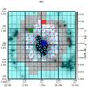 |
Fig. 1 Common grid (indicated by the black lines) generated for the SPIRE FTS observation overlaid on the star formation rate (SFR) map of M 83. The displayed SFR map has an equivalent spatial resolution (FWHM = 6.43′′), the same as the MIPS 24 μm broad-band image. Each pixel (black box) has a size of 15′′ × 15′′, which is equivalent to 330 pc × 330 pc at the distance to M 83. The SFR map is constructed from the far-ultraviolet (FUV) and 24 μm photometry maps following the calibration given in Hao et al. (2011; see Sects. 2.2 and 4.1 for more description). The magenta and cyan crosses indicate the pointings of the SLW and SSW detectors from all jiggle positions. The pixels masked by semi-transparent cyan color are outside the coverage of the SPIRE FTS maps presented in this work. The pixels masked by the semi-transparent gray color are truncated after the maps for observed lines are convolved to 42′′. The spectral energy distributions (SEDs) of three colored pixels, in blue, green, and red, indicating the nuclear, arm, and inter-arm regions, are displayed in Fig. 6 (see Sect. 3.2). The thick black lines are present as a guide to the labeled coordinates in the J2000 epoch. |
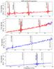 |
Fig. 2 Spectrum taken with the two central bolometers, SLWC3 (red) and SSWD4 (blue), from the center (blue pixel in Fig. 1) of the SPIRE FTS map of M 83. This spectrum has been corrected for the source-beam coupling effect with the method introduced in Wu et al. (2013). The source distribution is assumed to be a Gaussian profile with FWHM = 18′′, estimated from the overlap bandwidth of the two bolometers. The expected locations of the CO, [CI], and [NII] transitions listed in Table 1 are noted with the black dashed lines. |
Emission lines observed by the Herschel SPIRE FTS and the ground–based telescopes used in this work.
2.1.2. Map-making procedure
For each line observed by the Herschel FTS (see Table 1), a map is made based on the observed spectra in the frequency range, νline − 15 GHz <ν<νline + 15 GHz, where νline is the frequency of the emission line in the lab frame. For each detector, the observed spectrum is assumed to be uniform in a 15′′ × 15′′ area centered at the pointing of detector. The continuum is first removed from each observed spectrum prior to co-addition. The level of the continuum is simultaneously measured with a spectral model, which is a combination of a parabola (continuum) and a sinc (emission line) function, through the MPFIT procedure (Markwardt 2009). The spectrum assigned to each pixel is then computed as the error-weighted sum of each overlapping spectrum in proportion to its effective area in the pixel. Figures 3a and 4a demonstrate example maps of the spectra in the range of νline − 15 <ν<νline + 15 (GHz) for the transition, CO J = 4 − 3 and [NII ] 3P0 − 3P1, assigned to the pixels. We then fit the spectrum from each pixel with the spectral model to obtain a map of line fluxes (see Figs. 3b and 4b for an example).
As to the uncertainty estimate, although the pipeline gives statistical uncertainties which are computed as the variance of observed spectra from the total 16 scans for each detector, we found that the signal-to-noise ratio (S/N) is often over-estimated when considering only the pipeline-statistical uncertainty, judging from the noise level observed in the spectral data cube. This is especially the case when the central frequency of the line is close to the edge of the bandwidths. Because of this, we derive the random uncertainty from the residual after subtracting the continuum for each detector in the desired frequency range before co-addition, with exclusion of the central 10 GHz around the emission line so that the result of line measurement does not affect the uncertainty estimation. For each detector, the random uncertainty, which is to be propagated through the map-making, is generated based on the root-mean-square (rms) of the residuals. At each frequency grid, the random uncertainty is assigned by a random number generator assuming a normal distribution with the rms of the residuals as the 1σ. The uncertainties estimated with the rms of the residuals are termed “rms uncertainties” from here on.
The estimated absolute calibration uncertainty for the instrument is about 10% of the observed flux (Swinyard et al. 2014). The uncertainty assigned to each pixel is the summation in quadrature of the rms and calibration uncertainties. These uncertainties are propagated by the Monte-Carlo (MC) method with 300 iterations. Considering that the calibration uncertainty of each line and bolometer should not be independent, during one MC iteration, the percentage of calibration uncertainty is fixed for all the lines, and the rms uncertainty for each bolometer at each jiggle position is set to vary on every frequency grid. The final maps used in our analysis are presented in Figs. 3, 4, and Appendix A in the observed beam width (see Table 1). Interested readers should note that, toward the edge of the maps, the level of uncertainty increases (see Fig. A.10a), which sometimes makes the pixels on the edge appear falsely bright in Fig. A.10b.
 |
Fig. 3 Spatial distribution of the observed CO J = 4 − 3 line. a) continuum-removed coadded spectrum on every pixel within a range of 454 <ν< 468 GHz. The vertical axis in each pixel ranges between −9.8 × 10⁻¹⁹ and 5.4 × 10⁻¹⁹ W m-2 sr-1 Hz-1. b) measured CO J = 4 − 3 intensity distribution, in the unit of W m-2 sr-1, within the mapped region of M 83. Each pixel has size 15′′ × 15′′ or 330 pc × 330 pc. The spatial resolution of the map is 42′′. |
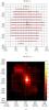 |
Fig. 4 Spatial distribution of the observed [NII] 205 μm line. a) continuum-removed coadded spectrum on every pixel within a range of 1452 <ν< 1467 GHz. The vertical axis in each pixel ranges between −1.7 × 10⁻¹⁷ and 9.3 × 10⁻¹⁷ W m-2 sr-1 Hz-1. b) measured [NII] 205 μm intensity distribution, in the unit of W m-2 sr-1, within the mapped region of M 83. Each pixel has size 15′′ × 15′′ or 330 pc × 330 pc. The spatial resolution of the map is 17′′. |
At the central pixel (marked by blue color in Fig. 1), the measured line intensities for the CO J = 4 − 3 and J = 6 − 5 transitions are (4.81 ± 0.66) × 10-9 and (7.13 ± 0.33) × 10-9 W m-2 sr-1 at the observed resolution, 42′′ and 29.3′′, respectively. At the same position, these two lines have been observed by the Caltech Submillimeter Observatory (CSO), and the measured intensities (converted from the main-beam temperature) for the CO J = 4 − 3 and J = 6 − 5 transitions are (1.2 ± 0.2) × 10-8 and (2.8 ± 0.2) × 10-8 at the spatial resolutions of 21.9′′ (Bayet et al. 2006). Following Bayet et al. (2006, Eq. (A.4) and Table 2), the intensities for the CO J = 4 − 3 and J = 6 − 5 transitions measured by CSO can be convolved to the SPIRE FTS resolution, resulting in (3.9 ± 0.6) × 10-9 and (1.69 ± 0.4) × 10-9 W m-2 sr-1, respectively. The intensity for CO J = 4 − 3 compares well between the two instruments, implying that the spatial distribution of CO J = 4 − 3 transition can be regarded as uniform within 42′′ in the nucleus. The SPIRE FTS measured intensity is smaller than the CSO measured one for CO J = 6 − 5 by a factor of 2.4, implying that the spatial distribution of the CO J = 6 − 5 transition should have a FWHM less than 29.3′′ and larger than 21.9′′.
In order to compare all the CO molecular and [CI] lines under a common spatial resolution, we convolve these maps to the largest beam size, ~42′′ (~910 pc), which is the beam FWHM of the CO J = 4 − 3 transition. The beam shape for the SSW can be well approximated by a pure Gaussian profile. However, the distribution of the beam profiles in the SLW is generally more complex and cannot be well described by a pure Gaussian except at the lowest frequency in its bandwidth. In order to construct kernels for convolving all the SPIRE FTS CO and [CI] maps, we adopt the parameters from fitting a 2D Hermite-Gaussian function to the beam profiles of the center detectors, SLWC3 and SSWD4. The off-center detectors are found to have similar beam profiles as the center ones (Makiwa et al. 2013), so we apply the same kernel to all bolometers on each map. The kernels used in the convolution process are constructed using the method described in Gordon et al. (2008) with the cutoff frequency in the Hanning function chosen so that the inclusion of the high spatial frequency is minimal. The pixels on the edge of each convolved map are truncated, so the effective FOV for the observed CO transitions at a common spatial resolution is as indicated by the unmasked pixels in Fig. 1.
2.2. Ancillary data
We compare the FTS data to the available ground-based CO observations, which include the maps of the J = 1−0 and J = 2 − 1 transitions observed with the Swedish-ESO Submillimetre Telescope (SEST) from Lundgren et al. (2004) and the J = 3−2 transition observed with the Atacama Submillimeter Telescope Experiment (ASTE) from Muraoka et al. (2009). Since our analysis is based on the point-source calibrated FTS data, we use the main-beam temperature for the CO transitions from the ground-based observations (see Table 1 for the information of the ground-based lines). We also calculate the SFR based on the far-ultraviolet (FUV) observation by the Galaxy Evolution Explorer (GALEX, Martin et al. 2005) and the 24μm observation by the Multiband Imaging Photometer for Spitzer (MIPS, Rieke et al. 2004). We derive dust properties based on the broad-band images from 3 to 500 μm observed by Spitzer and Herschel. One of the objectives of this work is to compare the atomic and molecular gas with dust properties. The atomic gas properties are derived from the data taken as part of The HI Nearby Galaxy Survey (THINGS, Walter et al. 2008). In this section, we provide a short summary of how the supplementary data are treated prior to comparison.
2.2.1. CO J = 1−0 and J = 2−1
The CO J = 1−0 and J = 2−1 observations of M 83 were done using the 15 m SEST during two epochs, 1989–1994 and 1997–2001 and presented in Lundgren et al. (2004). During the observations, the receivers were centered on the CO J = 1−0 and CO J = 2−1 lines (115.271 and 230.538 GHz, respectively), where the FWHM of the observed maps are 45′′ and 23′′, respectively. The CO J = 1−0 spectra were taken with 11′′ spacing, and the coverage was complete out to a radius of 4′20′′. The CO J = 2−1 spectra were taken with 7′′ spacing in the inner region of approximately 5′ × 3′ around the nucleus. The absolute uncertainty of the observations is about 10%. Lundgren et al. (2004) adopted relatively dense grid spacing, compared to the beamwidth, so that the spatial resolution of the data can be increased by using a MEM-DECONVOLUTION routine (maximum entropy method). The angular resolutions of the MEM-DECONVOLVED maps, which are adopted in this work, are ~22′′ and ~14′′ for the CO J = 1−0 and J = 2 − 1 maps, respectively. By convolving the MEM-DECONVOLVED data cube and comparing with the observed spectra, it has been verified that the MEM-DECONVOLVED results are reliable. Details of the data calibration and map-making for these two lines are described in Lundgren et al. (2004).
The pixel size of the CO J = 1−0 and J = 2−1 maps is 11′′ × 11′′. We first re-project these maps to the same world coordinate system (WCS) as the FTS maps, and convolve the re-projected maps to the equivalent spatial resolution of 42′′ to match the spatial resolution of the largest beam FWHM (42′′) of the SPIRE FTS. After convolution, the maps are resampled to the pixel size of the FTS maps (15′′ × 15′′) with the bicubic interpolation.
2.2.2. CO J = 3–2
The CO J = 3−2 observations of M 83 were made using the ASTE from 2008 May 15–21. The size of the CO J = 3−2 map is about 8′ × 8′ (10.5 × 10.5 kpc), including the whole optical disk. The half-power beam width (HPBW) of the ASTE 10 m dish is 22′′ at 345 GHz. The raw data were gridded to 7.5′′ per pixel, giving an effective spatial resolution of approximately 25′′. The absolute uncertainty of the observation is about 20%. Details of the data calibration and map-making can be found in Muraoka et al. (2009). We follow the same procedure described in Sect. 2.2.1 to reproject and convolve the map to the same pixel size and spatial resolution as the SPIRE FTS maps (15′′ × 15′′, 42′′).
2.2.3. FUV map
The FUV map of M 83 is made available as part of the GR7 (ops-v7_2_1) of GALEX. We obtain the FUV map through the Barbara A. Mikulski Archive for Space Telescopes (MAST1). The wavelength bandpass of these detectors in the FUV covers a range of 1400 to 1800 Å. The M 83 FUV map used in this work originates from the Nearby Galaxy Survey (NGS), which is a survey targeting nearby galaxies, including M 83, with a nominal exposure time of 1000 to 1500 s. In the case of M 83, the exposure time is 1349 s. The observed intensity and sky-background map is recorded in units of (photon) counts per second (CPS), and the conversion factor to units of erg s-1 cm-2 Å-1 is 1.40 × 10⁻¹⁵ erg s-1 cm-2 Å-1 CPS-1 (Morrissey et al. 2007).
The pixel size of the FUV map is 1.5′′ × 1.5′′ with a point spread function (PSF) of 4.2′′FWHM. We first re-project the FUV map to the same WCS as the FTS maps. For the purpose of analysis, we convolve the re-projected map to the equivalent spatial resolution of 22′′ to match the spatial resolution of the CO J = 1−0 map (see Sect. 4.1), and of 42′′ to match the spatial resolution of the CO J = 4−3 map (see Sect. 4.2.3). After that, the FUV map is resampled to the pixel size of the FTS maps (15′′ × 15′′) with the bicubic interpolation.
2.2.4. HI map
In order to derive the total gas mass in this work, we estimate the mass of atomic gas with the observations from the THINGS sample. All the galaxies in the THINGS sample are observed with the Very Large Array (VLA) in its B array configuration (baselines: 210 m to 11.4 km) with an addition of the D array (35 m to 1.03 km) and C array (35 m to 3.4 km) data to recover extended emission in the objects. The HI map of M 83 covers an area of 34′ × 34′. The final angular resolution of the HI map is 6′′. A detailed discussion of the data reduction procedure can be found in Walter et al. (2008).
We convert the observed HI map, from which the fluxes are calculated with a “natural weighting” scheme, with a conversion factor, 1.823 × 1018 cm-2 (Jy Beam-1 km s-1)-1, to derive the total HI column density, N(HI). The map of N(HI) is re-projected and convolved to match the pixel size (15′′ × 15′′) and angular resolution (42′′) of the FTS maps.
Broad-band image information.
2.2.5. Broad-band images
In order to derive the dust parameters, we collect the fully reduced Spitzer and Herschel broadband maps of M 83 previously presented by different studies. The 4 IRAC bands are those presented by Dong et al. (2008) and are public from the VizieR Catalogue Service. The MIPS 24μm image was presented by Bendo et al. (2012). Information for the broad-band images used in this work is listed in Table 2.
The PACS and SPIRE data are presented by Foyle et al. (2012) and are directly downloaded from the HeDaM website (Oliver et al. 2012). First, a median local background is subtracted from each map (see Table 2 for the aperture information). We then degraded the resolution to 42′′, corresponding to the SPIRE FTS spatial resolution at 650μm, which is the wavelength of the CO J = 4 − 3 transition. This step was performed using the method and the kernels provided by Aniano et al. (2011). Each map was then reprojected on the FTS common grid. Since the previous steps induce significant noise correlation between pixels, the statistical uncertainties for each photometry measurement are propagated through the data processing procedure. The uncertainty propagation is similar to the MC procedure described in Sect. 2.1.2. We perturb the value from each pixel of the photometry map (perturbed MC maps) by a normal distribution with the correspondent statistical uncertainty as the 1σ value. The final statistical uncertainty for each map is the standard deviation derived from the 300 perturbed MC maps. These uncertainties are then propagated through the SED fitting. The error on the dust SED parameters are the standard deviation of the distribution of the MC SED parameters.
3. Gas and dust modeling
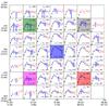 |
Fig. 5 Map of the CO SLEDs used in this study. Each pixel in this map is equal in its physical size to one pixel in Fig. 1. The CO transitions (in W m-2 sr-1) observed by the SPIRE FTS from unmasked pixels in Fig. 1 are shown here in blue (detected, S/N> 1) or red (upper limits). The dynamical range for each plotted SLED is the same as in Fig. 9. CO transitions of J = 1 − 0,2 − 1,3 − 2 observed by ground-based telescopes are shown as black triangles. All SLEDs that contain at least 2 detections with the SPIRE FTS are fitted with RADEX to obtain the best-fit parameters. The black solid line shows the SLED that is described by the best-fit parameters in RADEX with its best-fit Tkin and n(H2) labeled in each pixel, in units of K and cm-3 respectively. The data contained in the five color–masked pixels are highlighted in Fig. 9 and discussed in Sect. 4.2. |
3.1. Using RADEX to interpret the CO SLEDs
Our interpretation of the CO SLED is based on results computed by RADEX, a non-local thermal equilibrium (non-LTE) radiative transfer model with the assumption of local statistical equilibrium (van der Tak et al. 2007). The online manual2 of RADEX includes detailed discussions and derivation of the radiative transfer process in the model. We adopt the uniform-sphere approximation for the photon escape probability in our calculation and assume the cosmic microwave background (CMB) as the only background radiation field. The collision partners taken into account include H2 and e−, with the electron density set to 1 cm-3. We use the theoretical values of collisional cross-sections for CO, which were valid between 1 and 3000 K and calculated by Yang et al. (2010) based on the potential energy surfaces reported by Jankowski & Szalewicz (2005). In the computation, the line-width is assumed to be 50 km s-1, which is the average velocity width of the CO J = 3 − 2 map convolved to a spatial resolution of 42′′ within the central 1.5′ around the M 83 nucleus. The best-fit parameters are derived by comparing directly our intensities of CO transitions with the results from RADEX. In this section, we describe our approach of using RADEX as our data interpretation tool.
We first create a grid of RADEX-computed CO rotational line intensities based on the three main parameters: kinetic temperature (Tkin:K), H2 number density (n(H2):cm-3), and CO column density per velocity width (N(CO)/Δv:cm-2 (km s-1)-1). For each parameter, the input value varies along 101 uniformly spaced (in natural logarithmic scale) points within the range reported in Table 3. This gives 1 million SLEDs generated in the three dimensional parameter space.
RADEX parameters.
In order to efficiently search for the best-fit values in the parameter space, we create a function for each transition by linearly interpolating its values (Ik (J = i − j)) between points in a three–dimensional space, which is labeled Tkin, n(H2) and N(CO)/Δ v, with InterpolatingFunction of the ScientificPython library (v2.8). These thirteen functions (one for each line) are then called by MPFIT with the same set of parameters, Tkin, n (H2) and N(CO)/Δ v, to compute a SLED that best fits the observed values on a given pixel. The SLED generated by this method compares well with the results output by RADEX at each parameter grid. To ensure the best-fit parameters returned by MPFIT are indeed at the absolute minimum χ2 in the parameter space and not biased toward a local minimum due to our choice of initial parameters, we initiate the fitting process with parameters randomly selected within the range given in Table 3 and output one thousand sets of best-fit parameters and χ2 values given by MPFIT. We do this test with two scenarios such that the molecular cloud in the observed region (1) can be approximated by one temperature component (hereafter one-component fit); or (2) can be decomposed into two components of different temperatures (hereafter two-component fit). In reality, neither proposed scenario can describe all the observed molecular clouds, which might be tens or even hundreds in number, in detail. Given the limited spatial resolution of the instrument, the derived physical conditions should be treated as average values within the beam. We perform a one-component fit only at the pixels where there are more than 4 detections of CO transitions (S/N> 1) and a two-component fit where there are more than 7 detections, including the ground-based observations. Since this work includes multiple observed CO transitions, the S/N threshold is so chosen that the model can be the most constrained by as many observed lines simultaneously. The average S/N of the observed SLED is propagated with the MC method and reflected by the uncertainties of the derived physical parameters.
Based on the previous observational results from the nucleus of M 83, we expect the CO transitions of the SLED at the central pixel (marked by blue) of Fig. 5 to be dominated, on average, by a cold (Tkin ≲ 100 K) and dense (n(H2) >1000 cm-3) component (Israel & Baas 2001; Kramer et al. 2005; Bayet et al. 2006). We have observed that the one-component fits can often return best-fit parameters that are comparable to the values in the literature at its absolute minimum χ2. On the other hand, the results from two-component fits often are in two combinations: (1) a cold (Tkin< 100 K) but rather diffuse (n(H2) <100 cm-3) component with a column density higher than a warm (100 <Tkin< 1000 K) component which is of a reasonable density (n(H2) ~3000 cm-3); or (2) a cold and dense (n(H2) >105 cm-3) component with lower column density than a warm and diffuse (n(H2) <100 cm-3) component. The molecular gas density for the cold component predicted in the first scenario is too diffuse, while the cold-to-warm gas ratio predicted in the second scenario is too low. Neither scenario appears physical. To quantitatively test whether a second component is statistically necessary based on our data, we use the output χ2 and the corresponding degrees of freedom for both scenarios to perform an F-test, in which a ratio Fχ is computed to determine whether adding n terms of parameters to the original m terms can significantly improve the fit (Bevington & Robinson 2003) over the SLED. The ratio Fχ is defined as follows 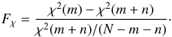 (1)For pixels with a sufficient number of detected lines for two-component fits, Fχ is generally less than 20, which corresponds to a 95% confidence level for comparing a model of 5 degrees of freedom with another of 2 degrees of freedom, and accordingly implies that the additional parameters contributed by adding a second component does not statistically improve the fit. Therefore, we derive our parameters using exclusively a single component model.
In order to better constrain the physical parameters, we attempt to include the two neutral carbon lines, [CI] 609 μm and [CI] 370 μm, observed by the SPIRE FTS in the fitting. Galactic observations with the Antarctic Submillimeter Telescope and Remote Observatory (AST/RO) have shown that the spatial distribution of [CI] 609 μm is similar to that of CO J = 1 − 0 within Milky Way (Martin et al. 2004). Assuming that the distributions of [CI] 609 μm and [CI] 370 μm are co-spatial with CO transitions on the ~330 pc scale, we assume the same kinetic temperature and molecular gas density in RADEX for [CI] as for CO but introduce the column density of [CI] (N(C)) as an additional parameter. With and without the inclusion of [CI] 609 μm and [CI] 370 μm, the derived values of n(H2) and Tkin are in agreement. However, similar to what Kamenetzky et al. (2012) have found in their study of the SPIRE FTS observation of M 82, N(C) is generally larger than N(CO) by a factor between 4 and 10 throughout the map. This result differs from the result derived from observations of Large Magellanic Cloud that N(C) is found to be 25% of N(CO) in 30 Doradus and ≈N(CO) in N159W (Pineda et al. 2012), hinting that the beam-filling factor for atomic carbon might be larger than CO transitions in our observations. Another possible explanation for the large N(C) /N(CO) ratio may be the high kinetic temperatures, which lead to a high value of the partition function, hence a large column density. On the other hand, recent studies of CO J = 1 − 0 in M 51 suggest that more than half of the CO J = 1 − 0 emission might originate on scales larger than 1.3 kpc (Pety et al. 2013). Assuming that the two lowest transitions of CO, J = 1 − 0 and J = 2 − 1 originate from more diffuse regions than other transitions, we have excluded these two lines when searching for the best-fit parameters with RADEX. In this scenario, the derived physical conditions remain consistent with the results derived with all available CO transitions in this study, which suggests that the dataset used in this work may not be sufficient to differentiate the origins of each transition spatially. We would also like to note that when the analysis in this work is based on the extended-source calibrated FTS data and the corrected antenna temperatures from the ground-based telescope, the derived physical conditions remain the same in general. However, since the extended-source calibrated data is smaller than the point-source calibrated data, the derived N(CO) is generally smaller when using the extended-source calibrated data.
Based on these results, we opt for the one-component fit scenario in our analysis with the inclusion of only the CO transitions, based on the point-source calibrated FTS data. Figure 5 shows the available SLEDs extracted from the SPIRE FTS observation, with their best-fit RADEX SLEDs indicated by solid black lines. The reduced χ2 for each fitted SLED is labeled on the individual pixel. The median reduced χ2 value is 0.76. The uncertainties estimated for the observed values are propagated through the MC method by randomly varying the SLEDs within a normal distribution and using the standard deviation of the best-fit parameters given by MPFIT as the 1σ uncertainty of the evaluated parameters. Further discussion of the CO SLEDs is presented in Sect. 4.2.
3.2. Dust properties
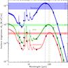 |
Fig. 6 Selected SEDs of M 83. They correspond to three pixels: one in the central region (Nucleus; blue); one on the spiral arm (Arm; green); one in the interarm region (Interarm; red). These three pixels are masked in the same colors in Fig. 1. The open circles with error bars are the observed photometry. The solid lines are the Galliano et al. (2011) model fit to these fluxes. The widths of the line indicate the levels of uncertainty of the model fit. The solid circles are the synthetic photometry computed from the model. The vertical dashed line shows the peak wavelength of the SED, which is an indication of the dust temperature. The horizontal stripes show the difference between the peak fluxes of the 7.7μm PAH feature and the FIR. They demonstrate that the PAH-to-FIR peak ratio, which can be translated to the PAH-to-dust mass ratio (fPAH), is similar in the arm and interarm regions, but is lower in the nucleus. |
One of our main objectives is to compare the physical properties derived from the CO SLEDs with the dust properties. In order to derive physical conditions for the dust, we fit the SED of each pixel of the regridded maps, using the dust model presented by Galliano et al. (2011). In brief, this model assumes that the distribution of starlight intensities heating the dust follows a power-law (Dale et al. 2001; Galliano et al. 2011). The parameters of this power-law are derived by the fitter, and are constrained by the actual shape of the infrared SED. It therefore accounts for the fact that several physical conditions are mixed within each pixel. This model uses the dust model and the Galactic grain composition presented by Zubko et al. (2004). We arbitrarily fix the charge fraction of polycyclic aromatic hydrocarbon (PAH) to 1/2, due to lack of constraints. The main parameters derived by the fitter include
-
1.
Mdust: the dust mass;
-
2.
⟨ U ⟩: the average intensity of the ISRF, normalized by the value in the solar neighborhood, 2.2 × 10⁻⁵W m-2 sr-1;
-
3.
fPAH: the PAH-to-dust mass fraction, normalized by the Galactic value (4.6%, Zubko et al. 2004).
To derive the uncertainties on the fitted parameters, we perform the SED fitting on each one of the perturbed MC maps (see Sect. 2.2.5) with the addition of the calibration uncertainties (see Table 2), following the method outlined in Galliano et al. (2011, Sect. 3.4).
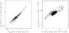 |
Fig. 7 Comparison between the results from this work and those from Foyle et al. (2012) after reprojecting the dust properties in Foyle et al. (2012) to the common grid used in this work. The left panel compares the dust masses from the two studies, pixel by pixel. The right panel compares the average intensity of the interstellar radiation field (⟨ U ⟩) with the dust temperature (Tdust) derived by Foyle et al. (2012). Tdust has been related to ⟨ U ⟩ with the relationship |

Three SEDs with best-fit parameters for three pixels selected from the nucleus (blue), arm (green), and interarm (red) are displayed in Fig. 6. The locations of these three pixels are marked by blue, green, and red colors in Fig. 1. The SEDs show difference in that the central region is on average hotter than the other regions, as the far-IR peaks at shorter wavelengths (indicated by vertical dashed lines). The far-IR component is also broader at the nucleus, as a consequence of the large variety of grain excitation conditions within the pixel. It indicates that the region likely contains one or several dense phases. For instance, if a region contains a molecular cloud, which is illuminated by a star cluster on one side, then the UV-edge of the cloud will be hot, and the temperature will decrease into the cloud, until it reaches a relatively cold temperature in the core. On the other hand, in a pixel containing mainly a diffuse phase, the far-IR SED will look isothermal, as the optical depth across the pixel will be moderate. Finally, the peak of the PAH features is much lower than the peak of the far-IR intensity at the nucleus, compared with that at the arm and interarm regions (indicated by the color stripes in Fig. 6). It indicates that fPAH is lower in the nucleus while it is close to the Galactic value in the rest of the map. This latter point is likely a sign that the nucleus hosts harder radiation fields, where PAHs are destroyed (Galliano et al. 2003, 2005; Madden et al. 2006; Gordon et al. 2008; Wu et al. 2011).
The FIR broad-band images from the FOV modeled here have been previously studied by Foyle et al. (2012). In Foyle et al. (2012), five broad-band images, including the PACS and SPIRE photometry data, are fitted with a single modified blackbody function, with an assumption that the emissivity (β) is equal to 2, to derive the dust mass and the equilibrium grain temperature (Tdust). In this work, we perform a more complex and realistic modeling, by accounting for the temperature mixing within each pixel, while Foyle et al. (2012) assumed an isothermal distribution of equilibrium grains. The model used in this work allows us to constrain the PAH mass fraction, which is interesting to be compared with the density of molecular gas (n(H2) derived from the CO SLEDs). To check the consistency between the results given in Foyle et al. (2012) and this work, the derived dust properties are compared in Fig. 7. The dust mass compares well throughout the FOV. However, comparison with Tdust is less straightforward, as we derive the intensity of ISRF, ⟨ U ⟩, within each pixel, instead. In the FIR/sub-mm regime, the relationship between ⟨ U ⟩ and Tdust can be written as  (β = 2). Moreover, Tdust is approximately 17.5K in the solar neighborhood (Boulanger et al. 1996), implying ⟨ U ⟩≃ (Tdust/ 17.5K)6. The two quantities are in general agreement, as shown on the right panel of Fig. 7. However, the relation is more scattered than with that for the dust masses, as ⟨ U ⟩ and Tdust are not exactly equivalent.
4. Results and discussion
The presentation of results is organized as follows. We first discuss the observed SFR in a global scale (~3.5′ in diameter) within our FOV (all pixels in Fig. 1, except the cyan-masked ones), and whether it is spatially related to the ionized gas tracers [NII] 205 μm, to [CI] 370 μm, and to ICO(1 − 0) in M 83. We then zoom in to a smaller region (~2.3′ in diameter) of the disk to discuss what we find with the observed CO transitions from the unmasked pixels in Fig. 1. We only derive physical parameters with RADEX from the pixels where more than four CO transitions are detected (see also Sect. 3.1) in the CO SLED, including the available ground-based observations, so the derived physical parameters are from an area approximately 1.3′ around the nucleus
4.1. Star formation rate and the fine-structure lines
The SPIRE FTS is by far the most sensitive instrument that can spatially resolve the [NII] 205 μm emission from an extragalactic object. In the bandwidth covered by the SPIRE FTS, the [NII] 205 μm is the most widely detected emission line from the observed region of M 83. From the spatial distribution, the emission of [NII] 205 μm peaks at the nucleus and extends from northeast to southwest in the FOV of the SPIRE FTS, where local maxima of ΣSFR can be identified in several spots. The fine-structure line of the atomic carbon, the [CI] 370 μm line (see Fig. A.11a), is also well detected over our FOV. Compared with the [NII] 205 μm emission, the spatial distribution of the [CI] 370 μm emission appears more concentrated around the nuclear region.
Tracing star formation with [NII] 205 μm has recently been proposed. Zhao et al. (2013) used a subsample of 70 spatially-unresolved galaxies from the Herschel open time project, Herschel Spectroscopic Survey of Warm Molecular Gas in Local Luminous Infrared Galaxies (LIRGs; PI: N. Lu), and found a relationship between the measured luminosity of [NII] 205 μm and the SFR, where the SFR in Zhao et al. (2013) was calibrated from the total infrared luminosity by using the relationship given in Kennicutt & Evans (2012). The calibration they found also well describes 30 star-forming galaxies, which are also included in their analysis. The star-forming galaxies in their analysis are taken from the sample in Brauher et al. (2008), where [NII] 205 μm is scaled from the [NII] 122 μm with a theoretical emission ratio of 2.6 (see Zhao et al. 2013, for more details). As to the atomic carbon emission, studies of nearby galaxies have revealed that the contribution of atomic carbon (traced by [CI] 609 μm) to the gas cooling stays comparable with the emission of CO J = 1 − 0 in a variety of environments, and it has been suggested that the atomic carbon emissions can be a good molecular gas tracer (Gerin & Phillips 2000; Israel & Baas 2002).
We investigate how the [NII] 205 μm and [CI] 370 μm emissions relate to ΣSFR and how their relationships compare with the existing one between ΣSFR and the CO J = 1 − 0 transition (Kennicutt et al. 2007), where ΣSFR is calibrated with the Hα and 24 μm emission. Because [CI] 370 μm is observed at a spatial resolution of ~38′′ while the spatial resolutions of the [NII] 205 μm and ICO(1 − 0) maps are comparable (~17′′ and 22′′, respectively), we compare the pixel-by-pixel values of the [NII] 205 μm surface brightness with the ΣSFR, and of the ICO(1 − 0) with ΣSFR at a spatial resolution of 22′′ and of the [CI] 370 μm surface brightness with the ΣSFR at a spatial resolution of 38′′. The ΣSFR is calculated from the FUV and 24 μm photometry maps of M 83 following the calibration given in Hao et al. (2011). Figure 8 shows that a general relationship exists between the values of [NII] 205 μm and the ΣSFR. Compared with the ICO(1−0), the surface brightness of [NII] 205 μm is around two orders of magnitudes higher, and the relationship between [NII] 205 μm and ΣSFR appears to have a shallower slope in Fig. 8. It is interesting to note that the values of [NII] 205 μm appear to reach a maximum around 2 × 10⁻⁸ W m-2 sr-1 (at a spatial resolution of 22′′) and range only over one order of magnitude while the values of ΣSFR range over about two orders of magnitude in the FOV.
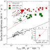 |
Fig. 8 Relationships between ΣSFR and [NII] 205 μm (red dots), between ΣSFR and [CI] 370 μm (green squares), and between ΣSFR and ICO(1−0) (black triangles). The sizes of the red dots and green squares are proportional to the S/N of the measured intensities. For [NII] 205 μm, the S/N ranges between 0.3 and 10.0 with a median value of 2.4. For [CI] 370 μm, the S/N ranges between 0.1 and 10.0 with a median value of 2.3. [NII] 205 μm and ICO(1−0) are compared with ΣSFR at a spatial resolution of 22′′, and [CI] 370 μm is compared with ΣSFR at a spatial resolution of 38′′. The red and black dashed lines indicate the SFR calibration converted from that given by Zhao et al. (2013) for [NII] 205 μm and by Kennicutt et al. (2007) for ICO(1−0), respectively. The box in the bottom right shows the integrated quantities of SFR and L[NII] 205 μm of M 83 from this work, with the dynamical range of both axes set to be the same as that in Zhao et al. (2013, Fig. 2). |
Zhao et al. (2013) have shown that the [NII] 205 μm luminosity holds the following relationship with the total SFR (calibrated with the total infrared luminosity, LIR) among a sample of 70 luminous infrared galaxies (LIRGs) and 30 star–forming galaxies 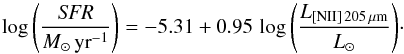 (2)After converting the total SFR to ΣSFR, and the [NII] 205 μm luminosity to surface brightness by using the pixel size (15′′, 330 pc) of the FTS maps, Eq. (2) is compared with our spatial results from M 83 as the red dashed line in Fig. 8. Equation (2) intersects with the data only at the high ΣSFR (ΣSFR> 1 M⊙ yr-1 kpc-2) end, but for regions with ΣSFR< 1 M⊙ yr-1 kpc-2, Eq. (2) does not fit well to the resolved data from M 83. This suggests that the relationship between ΣSFR and [NII] 205 μm described by Eq. (2) is dominated by active star-forming regions. In order to compare M 83 directly with the sample included in making the calibration in Eq. (2), we integrate the [NII] 205 μm surface brightness and ΣSFR from the observed region to obtain the L[NII] 205 μm and total SFR. The integrated value from M 83 is shown in the embedded plot in Fig. 8 where Eq. (2) (indicated by the red dashed line) well matches the values from M 83. This result shows that Eq. (2) can possibly be applied to galaxies in its global scale but cannot well describe the emission averaged from regions on ~300 pc scale. This is probably caused by the fact that [NII] 205 μm can also originate from more diffuse regions than the FUV and 24 μm emission due to its low critical density (~50 cm-3, main collisional partner: e−). This implies that the emission of [NII] 205 μm is more uniformly distributed within the galaxy than the adopted SFR indicator, even though its emission is still related to the star–forming activity. Indeed, Galactic observations with the Far-InfraRed Absolute Spetrophotometer (FIRAS) on the COsmic Background Explorer (COBE) have suggested that most of the Galactic [NII] 205 μm emission arises from from diffuse (ne< 100 cm-3) regions (Wright et al. 1991; Bennett et al. 1994). On the other hand, the relationship between the [CI] 370 μm emission and ΣSFR appears more linear. Within our FOV, the [CI] 370 μm surface brightness ranges over 1.5 orders of magnitude, which is comparable to the range of the values of ΣSFR. [CI] 370 μm has a critical density of ~1200 cm-3 (main collisional partners: H and H2), which is closer to the critical density of ICO(1 − 0) (~3000 cm-3, main collisional partners: H and H2), and its emission is brighter than ICO(1 − 0) by at least one order of magnitude. The [CI] 370 μm emission might originate from regions of similar physical conditions as ICO(1 − 0), and can potentially be a more reliable star formation tracer than the [NII] 205 μm emission.
Figure 8 also compares the ICO(1 − 0) with ΣSFR. The calibration of ΣSFR as a function of ΣH2 (estimated from the CO J = 1 − 0 intensity, ICO, Kennicutt et al. 2007) is indicated by the black dashed line (Eq. (3)). 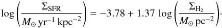 (3)We use N(H2) = 2.8 × 10²⁰ICO cm-2 (K km s-1)-1, the same conversion adopted by Kennicutt et al. (2007), to convert ΣH2 to the ICO(1 − 0) in Eq. (3). The relationship between the ΣSFR and ICO(1 − 0) observed in M 83 compares well with the spatially resolved study in M 51.
4.2. CO spectral line energy distribution
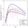 |
Fig. 9 Comparison of the CO SLEDs from the five color-masked pixels in Fig. 5. The five pixels are chosen to be the nucleus (blue) and four pixels that have equal distance (~1 kpc) from the nucleus at the northeast (green), southeast (magenta), northwest (gray), and southwest (red). The SLEDs and their best-fit from RADEX are shown in the same color. |
Before translating the observed quantities into physical parameters through RADEX, we first investigate how the intensity contributed by CO varies in different excitation states. Figure 9 shows the SLEDs from five pixels chosen from Fig. 5 at the nucleus (blue), and at the northeast (green), southeast (magenta), northwest (gray), and southwest (red), that have equal distance (~42′′, ~1 kpc; approximately the FWHM of the beam at the CO J = 4−3 transition) from the nucleus. From the nucleus, where the peaks of intensity of the CO transitions are found (see images in Appendix A), the average S/N for the detected CO transitions is ~10. The shape of the CO SLED from the nucleus of M 83 resembles the CO SLED observed from the nucleus of M 82, but with the peak intensity of CO transitions found at J = 4−3 (Panuzzo et al. 2010; Kamenetzky et al. 2012), hinting possibly softer radiation fields in this region, compared with the nucleus of M 82. The average S/N for the detected CO transitions from the four pixels around the nucleus is ~3, on average. The SLEDs along the bar (the northeast and southwest pixels) and from the southeast pixel appear to have similar shapes in that the highest intensity is found at J = 4−3. The SLED from the northwest pixel, on the other hand, shows higher intensities for CO transitions beyond J = 4−3, although it shows lower intensity at the CO J = 1−0 and J = 2−1 transitions than the three pixels from northeast, southeast and southwest. At the nucleus (the blue pixel in Fig. 5), where CO transitions are detected up to J = 12−11, the proportion of ICO(Jup = 4 to 8) to the total emitted intensity by CO is approximately 80%, assuming that the emission at Jup> 13, beyond the bandwidth of the SPIRE FTS, does not make a significant contribution. At the same pixel, the contribution of ICO(1−0) to the total emitted intensity is only ~1%. From Figs. 5 and 9, one can observe that, toward the nucleus, the intensities of higher excitation states (4 ≤ Jup ≤ 13) increase. Moreover, the fact that the peak intensity of the CO SLED from the northwest (gray pixel in Fig. 5) of the nucleus is found at higher-J transition (J = 6−5) implies that the radiation field may be harder toward this region.
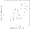 |
Fig. 10 Relationship between the ratio of intensities (in W m-2 sr-1) contributed by CO in the higher excitation states (J = 4−3 to J = 8−7) to that of CO at J = 1−0 versus ⟨ U ⟩. |
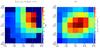 |
Fig. 11 Left: spatial distribution of the intensity ratio plotted in the y-axis of Fig. 10. Right: spatial distribution of ⟨ U ⟩, estimated by fitting the dust model to the SEDs over the FOV. |
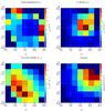 |
Fig. 12 Best-fit physical parameters, Tkin (top left), n(H2) (top right), N(CO) (bottom left), and pressure (bottom right) derived from Fig. 5 by RADEX. Figure 12d is a multiplication of Figs. 12a and b. |
To investigate how the emission of different CO transitions is affected by the local radiation field, we express the trend described above quantitatively in Fig. 10, in which we compare the ratio of total surface brightness contributed by J = 4−3 to J = 8−7 (ICO(Jup = 4 to 8), mid-J transitions) and ICO(1−0) with ⟨ U ⟩, which is a measure of average strength of ISRF. ICO(Jup = 4 to 8) covers most of the CO emission beyond the peak of the CO SLEDs within our FOV (see Fig. 5). Because the transitions with Jup ≥ 9 are detected only at the few central pixels (see Appendix A), we exclude them from ICO(Jup = 4 to 8) in our comparison. Figure 10 shows a clear increase of total emitted intensity contributed by transitions from higher excitation states when the total starlight intensity increases. This increase is in qualitative, although not quantitative, agreement to what is predicted by the PDR models (Kaufman et al. 1999; Wolfire et al. 2010; Le Petit et al. 2006). The spatial distribution of ICO(Jup = 4 to 8)/ICO(1 − 0) appears to increase toward the northwest of nucleus (see Fig. 11). This implies that the J = 1 − 0 transition alone may not be sufficient to represent the entire population of CO molecules. Emission of CO J = 1 − 0 is widely employed as an estimate of the total H2 column density (N(H2)). With spatially resolved CO transitions of higher excitation states, we can examine how the derived masses of molecular gas with RADEX compare to those with the intensities of CO J = 1 − 0, and how the physical parameters derived from Fig. 5 compare with dust properties and SFR.
Figure 12 shows the beam-averaged physical parameters derived from the observed CO SLEDs in Fig. 5. We would like to emphasize that the parameter N(CO) reported in this work actually includes an uncertainty due to our ignorance of the beam-filling factor at each transition. Constraining the beam-filling factor in the modeling introduces an additional parameter that is bound to be degenerate with N(CO), therefore the derived N(CO) should be viewed as the average value within the beam, which has a size of ~1 kpc. At the nucleus of Fig. 5 (the pixel highlighted in blue), the estimated Tkin, n(H2), and, N(CO), are 306 ± 63 K, 2630 ± 960 cm-3, and (9.49 ± 1.63) × 1017 cm-2, respectively. The CO transitions in this region have been observed by various ground-based telescopes. Israel & Baas (2001) report n(H2) = 1000 cm-3 and N(CO)/Δv = 1 × 1017 cm-2. Kramer et al. (2005) report n(H2) = 3000 cm-3 and N(CO)/Δv = 3.2 × 1016 cm-2. Bayet et al. (2006) report n(H2) = 6.5 × 105 cm-3 and N(CO)/Δv = 6 × 1016 cm-2. Our derived n(H2) and N(CO) are in general agreement with previously derived values in Israel & Baas (2001); Kramer et al. (2005) but different from the values reported in Bayet et al. (2006). The range of kinetic temperatures, Tkin, derived in this work, however, are higher than the values derived from previous observations (30 − 150 K, Israel & Baas 2001; 15 K, Kramer et al. 2005); and 40 K, Bayet et al. 2006). This discrepancy is largely due to our inclusion of transitions from higher excitation states, while previously reported values are based on CO SLEDs that include transitions between excitation states lower than or equal to J = 6 − 5. The remaining part of this Section is dedicated to the presentation of the physical parameters derived with RADEX from Fig. 5. Due to the inherent degeneracy of Tkin and n(H2) from RADEX, we quantitatively present them in this work as one parameter, the thermal pressure of molecular gas (Pth = Tkin·n(H2)). However, the spatial distributions of Tkin and n(H2) individually are discussed and compared with other physical parameters.
4.2.1. Column density of CO: emissivity of CO J = 1–0
The result shown in Fig. 10 implies that the emission of CO in the mid-J transitions, compared with that in the J = 1 − 0 transition, shows a steep increase with ⟨ U ⟩. This can be seen when one compares Fig. 11a with Fig. 11b. We define the emissivity of CO as the CO emission per molecule. The emissivity of CO in the J = 1 − 0 transition can be then expressed as ϵCO(J = 1 − 0) = ICO(1 − 0)/N(CO). We investigate how ϵCO(J = 1 − 0) varies spatially, using N(CO) derived with RADEX. Since ICO(1 − 0) is widely used as an estimate of total mass of molecular gas through a conversion factor, XCO, and N(CO) can be related to N(H2) through the abundance ratio of CO and H2 ([CO/H2]), ϵCO(J = 1 − 0) can be approximated as ![Mathematical equation: \hbox{$X_{\rm CO}^{-1}\ \mathrm{[CO/H_{2}]}^{-1}$}](/articles/aa/full_html/2015/03/aa23847-14/aa23847-14-eq385.png) . The spatial variation of ϵCO(J = 1 − 0) can therefore be approximately regarded as a combined variation of XCO and [CO/H2]. Figure 13 shows the relationship between ⟨ U ⟩ and ϵCO(J = 1 − 0). We derive an empirical relationship between ϵCO(J = 1 − 0) and ⟨ U ⟩ as follows:
. The spatial variation of ϵCO(J = 1 − 0) can therefore be approximately regarded as a combined variation of XCO and [CO/H2]. Figure 13 shows the relationship between ⟨ U ⟩ and ϵCO(J = 1 − 0). We derive an empirical relationship between ϵCO(J = 1 − 0) and ⟨ U ⟩ as follows:  (4)where ϵCO(J = 1 − 0) is in units of 10-26 erg s-1 sr-1 molecule-1, and ⟨ U ⟩ in units of 2.2 × 10⁻⁵ W m-2. The relation given in Eq. (4) is fitted to Fig. 13 with a reduced χ2 of 1.07.
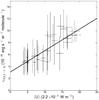 |
Fig. 13 Relationship between the emissivity of CO J = 1 − 0 and ⟨ U ⟩, derived by fitting the dust model to the SEDs. |
M 83 is known to have a shallow radial metallicity gradient (Dufour et al. 1980). A measurement from 11 targeted HII regions in M 83 show that the oxygen abundance, expressed as 12 + log (O/H), in the central ~80′′ of diameter (approximately the area shown in Fig. 12) is around 9.15 and varies between 9.07 and 9.25, which corresponds to a metallicity of ~2 Z⊙3 (Bresolin et al. 2002). Although [CO/H2] depends not only on the metallicity but also on the relative spatial distribution of CO and H2, the variation of the mass fraction of “CO-free” H2 might not be significant given that the metallicity within our FOV is super solar and has a shallow radial gradient (Wolfire et al. 2010). If one assumes that the relative abundance of CO to H2 is uniform within our FOV, the relationship observed in Fig. 13 implies that XCO decreases as ⟨ U ⟩ increases. This relationship is similar to the existing relationship between αCO, the molecular-mass-to-intensity ratio, and luminosity of CO J = 1 − 0 transition (LCO), in which a decreasing trend in αCO is found when the LCO of giant molecular clouds (GMC) in the Milky Way increases (Solomon & Rivolo 1987; Bolatto et al. 2013). With a sample of 26 nearby galaxies, Sandstrom et al. (2013) have found that αCO decreases when ⟨ U ⟩ increases when comparing the dust SEDs with ICO(1 − 0) at the ~1 kpc scale, assuming a metallicity-dependent gas-to-dust mass ratio. Lower values of XCO have also been observed from local ULIRGs (Papadopoulos et al. 2012) and mergers (Narayanan et al. 2011).
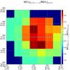 |
Fig. 14 Spatial distribution of M(H2)J = 1 − 0/M(H2)N(CO) from the area where CO SLEDs are modeled with RADEX. |
The spatial variation of ϵCO(J = 1 − 0) can also be regarded as the variation of the mass of H2 derived from two different approaches. We define M(H2)J = 1 − 0 as the mass of H2 derived from ICO(1 − 0) with the Galactic XCO value, 2 × 1020 cm-2 (K km s-1)-1 (Strong & Mattox 1996), and M(H2)N(CO) as the total H2 mass converted from the estimated N(CO) with RADEX in this work, assuming [CO/H2] = 2.7 × 10⁻⁴, which is comparable to the solar abundance and is measured from the nearby Flame Nebula, NGC 2024 (Lacy et al. 1994). Figures 11b and 14 spatially compare the distribution of ⟨ U ⟩ and M(H2)J = 1 − 0/M(H2)N(CO) ∝ ϵCO(J = 1 − 0). As suggested by Fig. 13, ⟨ U ⟩ and M(H2)J = 1 − 0/M(H2)N(CO) generally resemble each other in their spatial distribution. Values of M(H2)J = 1 − 0/M(H2)N(CO) in Fig. 14 have an average of 2.4 and range between 1.6 and 3.7. Given that M(H2)J = 1 − 0 and M(H2)N(CO) are estimated from two different approaches, the adopted conversion factors generally agree with each other. However, our result suggests that, on the local scale, the ISRF might have a role in determining both XCO and [CO/H2], whether through direct or indirect effect, and that one needs to be cautious when deriving the XCO factor based on the CO transitions studied in this work.
4.2.2. Column density of CO: gas-to-dust mass ratio
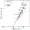 |
Fig. 15 Comparison of the dust molecular gas masses estimated in M 83. Points with error bars are the values derived using the Herschel SPIRE FTS data. Blue points indicate the values estimated with ICO(1 − 0) (XCO = 2 × 1020 cm-2 (K km s-1)-1) when there is no available data from FTS observation. Red crosses indicate the values used in Foyle et al. (2012), in which the G/D is estimated to be 84 ± 4 (dashed line) within M 83. |
The derived N(CO) also provides an alternative way to estimate the gas-to-dust mass ratio (G/D) in M 83. Figure 15 shows the relationship between the dust and total gas mass surface density in M 83 from the entire area of Fig. 1. Foyle et al. (2012) has estimated an average G/D = 84 ± 4 (the dashed line in Fig. 15) within an area of 12′ × 12′ centered at the M 83 nucleus, using the same XCO factor as used in this work. They derive the dust mass with a modified blackbody fit to the two Herschel PACS and three SPIRE broad band images at 70, 160, 250, 350, and, 500 μm. For the H2 mass, they scale the observed CO J = 3 − 2 map to match the CO J = 1 − 0 map and derive the H2 mass from the scaled J = 3 − 2 observation. The HI gas mass in Foyle et al. (2012) is derived from the M 83 observation in the THINGS program, which is the same map used in this study. The data points from Foyle et al. (2012) are shown as red crosses in Fig. 15. We add the HI gas mass to M(H2)N(CO) for the points with S/N> 1 for N(CO) to derive the total hydrogen gas mass. The total gas mass, including the helium contribution, is then calculated as 1.36 times the total hydrogen gas mass4. The G/D estimated from the CO SLEDs is 106 ± 47 (the black points with error bars in Fig. 15), which is similar to the values found within central 1 kpc of radius in Foyle et al. (2012). Because the available pixels in Fig. 5 only cover a ~1.5′ × 1.5′ area around the M 83 nucleus, for pixels that do not have sufficient S/N data observed by the SPIRE FTS, we estimate the total gas mass with M(H2)J = 1 − 0 (blue points in Fig. 15). The total G/D we estimated from the entire area, including the cyan-masked pixels in Fig. 1, is 93 ± 19, which is in general agreement with the value estimated in Foyle et al. (2012) and is about half of the G/D estimated in the diffuse ISM of the Milky Way (Zubko et al. 2004). This result is consistent with the metallicity of the central region of M 83 being twice solar, as it implies that the dust-to-metal mass ratio is similar to the Galactic value.
4.2.3. Column density of CO: gas depletion time
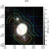 |
Fig. 16 Contours of N(CO), derived in this work, overlaid on the SFR map. The contours are spaced by 1.5 × 1017 cm-2. The red and blue contours correspond to the highest (1.2 × 1018 cm-2) and lowest (3 × 1017 cm-2) values of N(CO) (see also Fig. 12c). |
The analysis of the relationship between gas mass and SFR has given indirect evidence that nearby spiral galaxies are forming stars with a constant gas depletion time (Bigiel et al. 2008, 2011; Leroy et al. 2008, 2013). Using a sample of 30 disk, non-edge-on (inclination≲75°) and spatially resolved (down to ~1 kpc) galaxies, Bigiel et al. (2011) found a linear relationship between ΣH2 and ΣSFR, which gives a constant molecular gas depletion time ( ) of 2.35 ± 0.24 Gyr with 1σ scatter 0.24 dex. This sample spans an oxygen abundance range of 8.36 ≲ 12 + log (O/H) ≲ 8.93 and a mass range of 8.9 ≲ log (M∗/M⊙) ≲ 11.0, which are compatible with the global properties of M 83, which has a stellar mass of log (M∗/M⊙) ~ 10.9 (Jarrett et al. 2013). As already discussed in Sect. 4.1, we have found that the ΣH2 (derived with ICO(1 − 0)) and the ΣSFR are related spatially within M 83. Figure 16 shows this relationship spatially with N(CO) derived with RADEX. It is clear that N(CO) has a very similar spatial distribution to that of the SFR map. We now revisit the quantitative relationship found in Bigiel et al. (2011) but with the addition of M(H2)N(CO), in Fig. 17.
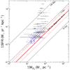 |
Fig. 17 Comparison of the molecular gas mass and SFR surface density estimated in M 83. Points with error bars are the values derived using the Herschel SPIRE FTS data. Blue points indicate the values estimated with ICO(1 − 0) (XCO = 2 × 1020 cm-2 (K km s-1)-1) when there is no available data from FTS observation. The 2.35 Gyr, which is the gas depletion time found within 30 nearby spatially resolved spiral galaxies in Bigiel et al. (2011), is shown as the solid line, with its 1σ scatter marked by the red dash-dotted lines. |
Within the area of 3′ × 3′ around the nucleus, we found an average (molecular) gas depletion time of 1.13 ± 0.6 Gyr, estimated from the combination of M(H2)N(CO) and M(H2)J = 1 − 0. This number is smaller than the result previously found (~2.35 Gyr, shown as the red solid line with the 1σ values indicated by the red dotted lines in Fig. 17). The smaller gas depletion time found in this work can be explained by the fact that the map covered in Fig. 16 is dominated by M 83’s starburst nucleus region, within which strong starburst activity is found accompanied by a concentration of X-ray sources (Soria & Wu 2002). It can be that the depletion of molecular gas by star formation is more efficient in this region, or that the molecular gas, traced by CO, is dissociated through other mechanisms. Figure 17 also shows that ΣH2 appears to reach a maximum at ~100 M⊙ pc-2. The appearance of the ΣH2 saturation at ~100 M⊙ pc-2 can be caused by two reasons. First, the N(CO) derived in this work may underestimate the total CO column density, due to the fact that the N(CO) is an averaged property of cold and warm CO molecular gas together over a large scale (~1 kpc). However, we would like to point out that in Fig. 17, M(H2)J = 1 − 0 (blue points) also shows the saturation toward the higher SFR regions. Second, whether through direct or indirect effects, when the SFR increases, self-shielding of CO might become less efficient so that the molecules are dissociated while H2 molecules can still remain in the molecular state due to more efficient self-shielding (van Dishoeck & Black 1988; Liszt & Lucas 1998; Wolfire et al. 2010; Levrier et al. 2012). Based on these two reasons, the observed “saturation” of molecular mass at ~100 M⊙ pc-2 does not directly imply a maximum value of ΣH2 when ΣSFR increases.
4.2.4. Pressure: excitation of molecular CO
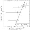 |
Fig. 18 Relationship between Pth, derived from CO SLEDs, and ⟨ U ⟩, derived from the SEDs. The plotted points all have S/N> 1 for the derived Pth. A linear relationship is found between Pth and radiation pressure (Prad). This relationship is shown in the box on the lower right of the graph. |
Similar to the spatial distribution of ICO(Jup = 4 to 8)/ICO(1 − 0), the spatial distribution of Pth appears to increase toward the northwest of nucleus, where peak of ⟨ U ⟩ is found. Figure 18 compares Pth and ⟨ U ⟩ pixel-by-pixel, wherever the derived Pth has S/N> 1. A general relationship between Pth and ⟨ U ⟩ appears that, if expressing ⟨ U ⟩ as radiation pressure (Prad = ⟨ U ⟩ /3 c, where c is the speed of light), the pressure of the molecular gas is approximately thirty times the average radiation pressure generated by the ISRF. This means that the energy density of the ISRF is less than 5% of the kinetic energy density of molecular gas, so that it is unlikely that ⟨ U ⟩ can supply the energy to maintain the observed CO transitions in M 83. The transitions of CO molecules observed by the SPIRE FTS may be tracing other radiation sources than the ISRF. Similarly, studies of the nearby galaxies, M 82 and Arp 220, also suggest that the CO transitions observed by the SPIRE FTS cannot be explained with PDR alone and still be consistent with solutions from RADEX (Rangwala et al. 2011; Kamenetzky et al. 2012). However, we would also like to point out that, by studying the CO transitions in the nearby interacting system, the Antennae, with the SPIRE FTS, Schirm et al. (2013) conclude that the ISRF and the radiation generated by turbulence due to the ongoing merger or supernova are both likely responsible for the observed CO transitions. The energy source traced by the observed CO transitions should also depend on the radiation environments.
The pressure of the molecular gas derived in this work is 1.63 × 10⁵<Pth< 2.12 × 106 cm-3 K, which is consistent with the estimated pressure of the warm neutral medium (WNM) associated with SNR, based on the shock models of Dopita & Sutherland (1996) and the radiative shock theory. Assuming a shock velocity of 200 km s-1 and a typical temperature of the WNM (~5000 K), Dopita et al. (2010) derive from the observed Hα luminosity of SNR in the radiative phase that the range of ISM pressures in M 83 is of the order 5 × 10³<P< 1.5 × 106 cm-3 K. Although the estimated pressure in Dopita et al. (2010) spans a larger range than the values derived from the CO SLED, it shows that radiative shocks associated with SNRs cannot be excluded from the possible energy sources traced by the observed CO transitions. Following similar analysis as in Maloney (1999, Eq. (14)), we estimate the energy released by supernovae to be LSN = 1.5 × 10⁸L⊙ in the nucleus of M 83, with a supernova rate of 0.02 yr-1 estimated at the M 83 nucleus (Dopita et al. 2010). The total CO luminosity of the M 83 nucleus (blue pixel in Fig. 5), calculated from ICO(Jup = 4 to 8), is approximately 4.9 × 10⁴L⊙. This represents less than 0.5% of LSN and makes radiative shock produced by supernovae a possible energy source to supply the necessary energy budget for the observed CO transitions.
Another interesting feature we observe from the map of Pth is shown in Fig. 19 where the contours of Pth are overlaid on the SFR map. There is a clear gradient of Pth pointing from the southeast of the SFR nucleus (~(3.5 ± 2.0) × 105 cm-3 K, magenta cross in Fig. 19) toward the northwest (~(9.9 ± 1.7) × 105 and ~(2.1 ± 1.5) × 106 cm-3 K, green and cyan crosses in Fig. 19) within a physical scale of ~1 kpc. As already pointed out in Harris et al. (2001), based on the determined age of young star clusters with EW(Hα), they conclude that the starburst in M 83 generally propagates from the southern end (aged around or older than 10 Myr) toward the northern end (aged around or less than 5 Myr) of the nucleus, within a range of ~300 pc. The increase of pressure from the magenta toward green crosses in Fig. 19 is in agreement with this picture. The increase of pressure from magenta toward cyan crosses also traces the alignment of the observed radio sources, which are distributed along the green arrow in Fig. 19, from the optical nucleus toward sources #32, 30, 29, and 28 listed in Maddox et al. (2006; hereafter R32, etc.). The locations of these sources are marked by the cyan diamonds in Fig. 19 from the nucleus along the green arrow, respectively. Although Maddox et al. (2006) suggest that the source R28 in their observation is likely the nucleus of a background radio galaxy with its radio lobes traced by the radio sources R29 and R27, Dottori et al. (2010) propose that R28, which coincides with an X-ray source observed with the ACIS-S3 chip of the Chandra X-ray Observatory (labeled #39 in Soria & Wu 2003), might be a local emission from M 83, based on the low redshift (z ≪ 1) derived from the marginally detected Fe-K line by Chandra. There is a chance that the pressure gradient is linked to the observed radio-jet.
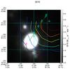 |
Fig. 19 Graph showing the contours of Pth on the SFR map. The gray scale of SFR is recorded in the colorbar to the right. The contours of Pth ranges between 4 × 10⁵ (blue) and 2.4 × 106 cm-3 K (red) and have spacings equal to 4 × 105 cm-3 K. The crosses mark the locations of three pixels chosen from Fig. 5 (see text for more details). The four cyan diamonds mark the locations of four radio sources observed in Maddox et al. (2006). |
Although due to the large beam size of the SPIRE FTS the derived values of pressure along the green arrow in Fig. 19 cannot be regarded as fully independent of each other, the general observed trend and its coinciding with previous findings in the literature are encouraging. Similar studies using spatial distributions of pressure with higher spatial resolution will potentially reveal the effects of stellar feedback on molecular gas.
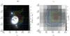 |
Fig. 20 Comparison of derived n(H2) contours with the SFR (left) and fPAH (right) images. In both figures, the contours for n(H2) are spaced by 400 cm-3, with the red and dark blue colors correspond to the highest (2800 cm-3) and lowest (400 cm-3) values. The two crosses in the left figure indicate the locations for the optical nucleus (magenta) and the young (age ≲3 Myr) star clusters (blue). The values of fPAH in the right figure are normalized by the Galactic value, which is 4.6% (see Sect. 3.2). |
4.2.5. Off-centered n(H2) density peak
Comparing with the SFR map, Fig. 20a shows that the peak of the distribution of n(H2) is slightly offset toward the northwest of the SFR nucleus. Although the offset from the optical nucleus (the magenta cross in Fig. 20a, Thatte et al. 2000) observed in our work is ~25′′, which is smaller than the beam FWHM at CO J = 4−3 (~42′′), considering the bolometer spacing of SLW (~12.7′′) from a complete Nyquist sampled map, this offset is likely to be physical. We have noted that, in Crosthwaite et al. (2002), a small offset of the peak of CO J = 1 − 0 emission, observed with the former NRAO 12 m telescope at Kitt Peak, from M 83’s optical nucleus (from a B-band image) is also present. Sakamoto et al. (2004) also observe from the CO J = 2 − 1 map that its redshifted peak is separated from the blueshifted peak by approximately 10′′. Using the Hubble Space Telescope Wide Field Planetary Camera 2, Harris et al. (2001) has determined the age of 45 star clusters within the 300 pc of M 83’s optical nucleus based on the comparison of measured optical colors with predictions made by stellar population synthesis models generated with Starburst99 (Leitherer et al. 1999). Within their sample, they found four heavily extincted objects, whose ages are difficult to determine from the model prediction. Two of these four clusters, situated close to each other, aged 3.07 and 2.22 Myr (#5 and #7 in Harris et al. 2001, shown as a blue cross in Fig. 20a) based on the measured equivalent widths of Hα, are found close to the peak of n(H2), derived with the SPIRE FTS. As pointed out in Sect. 3.2, the result from dust SED modeling reveals that fPAH is lower near the nuclear region than elsewhere in M 83, within our FOV, hinting at the possibility of the destruction of PAH in the nucleus. The derived fPAH from this work is shown as the background image in Fig. 20b. At the pixel where the highest n(H2) is derived (3000 ± 2000 cm-3), the value of fPAH is ~0.45, which is equivalent to a mass fraction of ~2% with respect to dust, while fPAH is close to one elsewhere. This is also one of the pixels where CO transitions are detected up to J = 10 − 9. The lowest value of fPAH within our map is ~0.41 and is found at the north adjacent pixel from the n(H2) peak. Since n(H2) and fPAH are derived independently of two different methods and datasets, the observed northwestern offsets of the lowest value of fPAH and the peak of CO emission from the optical nucleus are likely tracing very recent (≲3 Myr) starbursts, which are heavily extincted in FUV and optical. It hints that the CO transitions more energetic than J = 9 − 8, which are only detected in the nucleus of M 83, may be tracing radiative mechanisms directly or indirectly associated with very recent starbursts, such as shocks produced by supernovae or stellar winds.
5. Concluding remarks and summary
The Herschel SPIRE FTS uses a pioneering design to simultaneously observe a broad range of CO transitions in spectral imaging mode. Such a design enables us to derive the physical properties of molecular gas in a macroscopic field of view. Although the available spatial and spectral resolutions of the instrument are insufficient to differentiate the dynamics of individual molecular clouds in galaxies beyond the Milky Way, the main strength of such observations lies in its ability to provide a broad and average view of the physical conditions of the molecular gas properties traced by CO. Up to this point, our understanding about interstellar molecular gas properties is still limited. There are still many open questions, such as: what are the limitations of using observed CO to trace the states of molecular gas? What is the relationship between the formations of molecular clouds and stars? Results derived from observations by the SPIRE FTS help pave the way for the current and future studies of gas and dust, whether using ground-based telescopes, such as ALMA and JCMT, airborne observatories, such as SOFIA, or space observatories, such as JWST and SPICA. We summarize our findings from this work in the following six points:
-
1.
Comparing the star formation surface density (ΣSFR) with[NII] 205 μm, [CI] 370 μm, and surface brightness of CO J = 1 − 0 (ICO(1 − 0)), wefind that the previously established relationship be-tween ΣSFR and ICO(1 − 0) can also well describe the observations inM 83. On a global scale, the integrated SFR and L[NII] 205 μmfrom M 83 agree with the calibration proposedby Zhao et al. (2013). However,the relationship between ΣSFR and [NII] 205 μm appears to be affected by local con-ditions within M 83 such that the regions withlower ΣSFR show higher [NII] 205 μm than that given by the calibration. On the otherhand, the observed spatially resolvedlinear relationship between [CI] 370 μmand ΣSFR implies that, compared with the results from [NII] 205 μm, [CI] 370 μm can potentiallybe a better SFR tracer.
-
2.
Based on the derived N(CO) from the CO SLED map, we find a relationship between emissivity of CO molecules in the J = 1 − 0 state (ϵCO(J = 1 − 0) = ICO(1 − 0)/N(CO)) and ⟨ U ⟩, the strength of the interstellar radiation field, determined from fitting the dust model to the SEDs. The increasing relationship of ϵCO(J = 1 − 0) and ⟨ U ⟩ implies a decreasing relationship between XCO and ⟨ U ⟩.
-
3.
We convert N(CO) to mass of H2 and derive gas-to-dust ratios mass of 77 ± 33 within the central 1 kpc (in radius) of M 83 and 93 ± 19 from the region enclosed by the inner spiral arms, which are consistent with the results from Foyle et al. (2012). The gas depletion time in M 83 is estimated to be 1.13 ± 0.6 Gyr, which is smaller than that estimated statistically from 30 nearby galaxies (2.35 Gyr, Bigiel et al. 2011). This difference can be caused by either the limitation of the derived N(CO) to trace mass of H2 or the strong starburst within the M 83 nucleus.
-
4.
Overall, the derived molecular gas pressure is consistent in its values with the estimates from Hα photometry based on the shock models of Dopita & Sutherland (1996). We find that the molecular gas pressure (Pth) is generally linearly related to the radiation pressure of the average starlight intensity (Prad). This relationship can be expressed as Pth = 30 Prad, which indicates that the ISRF in M 83 alone is insufficient to supply the energy budget for the observed CO transitions in the SPIRE FTS.
-
5.
Our calculation shows that it requires less than 0.5% of supernovae luminosity (LSN) to power the observed luminosity of CO in M 83. This makes the CO transitions observed with the SPIRE FTS possible tracers for radiative shocks of supernova remnants. We also observe a gradient of molecular gas pressure pointing from the M 83 nucleus toward 1 kpc northwest of it. This direction is generally consistent with the observed propagation of the starburst pointed out by Harris et al. (2001). The gradient of molecular gas pressure also follows the observed “jet-like” distribution of radio sources (Maddox et al. 2006), whose location, whether they are local or in the background, is still under debate (Dottori et al. 2010). Because our results are restricted by the spatial resolution of the instrument, we are not able to pinpoint the association of the gradient with its cause(s). However, the coincidence of these results demonstrates the strong potential in studying stellar feedback with spatial distributions of pressure.
-
6.
From the derived map of n(H2), we find an offset of the molecular density peak from the optical nucleus by ~25′′. This offset traces well the decrease in PAH-to-dust mass fraction (fPAH) as well as two heavily extincted young clusters in its location. We conclude that the observed CO transitions are possibly tracing the radiative mechanisms directly or indirectly associated with very recent starbursts.
Online material
Appendix A: Line maps observed by the Herschel SPIRE FTS in M 83
We show the observed maps of the lines listed in Table 1 by the SPIRE FTS. All the maps are displayed in the observed spatial resolution and in the units of W m-2 sr-1 GHz-1 (line profile maps) and W m-2 sr-1 (integrated intensity maps).
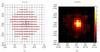 |
Fig. A.1 Illustration of the spatial distribution of the observed CO J = 5 − 4 line. Left panel: continuum-removed coadded spectrum on every pixel within a range of 568 <ν< 582 GHz. The vertical axis in each pixel ranges between −1.5 × 10⁻¹⁸ and 8.2 × 10⁻¹⁸ W m-2 sr-1 Hz-1. The color map on the right is in the units of W m-2 sr-1. |
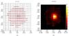 |
Fig. A.2 Illustration of the spatial distribution of the observed CO J = 6 − 5 line. Left panel: continuum-removed coadded spectrum on every pixel within a range of 683 <ν< 698 GHz. The vertical axis in each pixel ranges between −1.5 × 10⁻¹⁸ and 8.2 × 10⁻¹⁸ W m-2 sr-1 Hz-1. The color map on the right is in the units of W m-2 sr-1. |
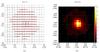 |
Fig. A.3 Illustration of the spatial distribution of the observed CO J = 7 − 6 line. Left panel: continuum-removed coadded spectrum on every pixel within a range of 798 <ν< 813 GHz. The vertical axis in each pixel ranges between −9.0 × 10⁻¹⁹ and 5.0 × 10⁻¹⁸ W m-2 sr-1 Hz-1. The color map on the right is in the units of W m-2 sr-1. |
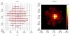 |
Fig. A.4 Illustration of the spatial distribution of the observed CO J = 8 − 7 line. The Left panel: continuum-removed coadded spectrum on every pixel within a range of 913 <ν< 928 GHz. The vertical axis in each pixel ranges between −6.3 × 10⁻¹⁹ and 3.5 × 10⁻¹⁸ W m-2 sr-1 Hz-1. The color map on the right is in the units of W m-2 sr-1. |
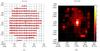 |
Fig. A.5 Illustration of the spatial distribution of the observed CO J = 9 − 8 line. Left panel: continuum-removed coadded spectrum on every pixel within a range of 1028 <ν< 1042 GHz. The vertical axis in each pixel ranges between −1.3 × 10⁻¹⁸ and 7.1 × 10⁻¹⁸ W m-2 sr-1 Hz-1. The color map on the right is in the units of W m-2 sr-1. |
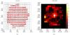 |
Fig. A.6 Illustration of the spatial distribution of the observed CO J = 10 − 9 line. Left panel: continuum-removed coadded spectrum on every pixel within a range of 1143 <ν< 1157 GHz. The vertical axis in each pixel ranges between −1.1 × 10⁻¹⁸ and 6.1 × 10⁻¹⁸ W m-2 sr-1 Hz-1. The color map on the right is in the units of W m-2 sr-1. |
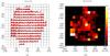 |
Fig. A.7 Illustration of the spatial distribution of the observed CO J = 11 − 10 line. Left panel: continuum-removed coadded spectrum on every pixel within a range of 1258 <ν< 1272 GHz. The vertical axis in each pixel ranges between −9.2 × 10⁻¹⁹ and 5.1 × 10⁻¹⁸ W m-2 sr-1 Hz-1. The color map on the right is in the units of W m-2 sr-1. |
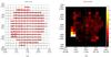 |
Fig. A.8 Illustration of the spatial distribution of the observed CO J = 12 − 11 line. Left panel: continuum-removed coadded spectrum on every pixel within a range of 1372 <ν< 1387 GHz. The vertical axis in each pixel ranges between −8.9 × 10⁻¹⁹ and 4.9 × 10⁻¹⁸ W m-2 sr-1 Hz-1. The color map on the right is in the units of W m-2 sr-1. |
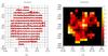 |
Fig. A.9 Illustration of the spatial distribution of the observed CO J = 13 − 12 line. Left panel: continuum-removed coadded spectrum on every pixel within a range of 1487 <ν< 1502 GHz. The vertical axis in each pixel ranges between −9.7 × 10⁻¹⁹ and 5.4 × 10⁻¹⁸ W m-2 sr-1 Hz-1. The color map on the right is in the units of W m-2 sr-1. |
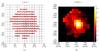 |
Fig. A.10 Illustration of the spatial distribution of the observed [CI] 609 μm line. Left panel: continuum-removed coadded spectrum on every pixel within a range of 484 <ν< 499 GHz. The vertical axis in each pixel ranges between −3.9 × 10⁻¹⁹ and 2.2 × 10⁻¹⁸ W m-2 sr-1 Hz-1. The color map on the right is in the units of W m-2 sr-1. |
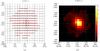 |
Fig. A.11 Illustration of the spatial distribution of the observed [CI] 370 μm line. Left panel: continuum-removed coadded spectrum on every pixel within a range of 801 <ν< 815 GHz. The vertical axis in each pixel ranges between −8.8 × 10⁻¹⁹ and 4.9 × 10⁻¹⁸ W m-2 sr-1 Hz-1. The color map on the right is in the units of W m-2 sr-1. |
12 + log (O/H)⊙ = 8.69 (Asplund et al. 2009).
[He/H] ~ 10%.
Acknowledgments
We would like to thank the anonymous referee for the constructive comments. R.W. would like to thank Dr. Estelle Bayet, Dr. Kelly Foyle, Dr. Andreas A. Lundgren, Dr. Kazuyuki Muraoka and Dr. Glenn R. Petitpas for generously sharing their data, and Dr. George Bendo, Dr. Horácio Dottori, and Dr. Eric Pellegrini for fruitful discussions. Special thanks go to the members of the Herschel SPIRE Instrument Control Centre (ICC) for their continuous support throughout the project. This research was supported in part by the Grant-in-Aid for Scientific Research for the Japan Society of Promotion of Science (140500000638). This research was also supported by grants from the Canadian Space Agency and the Natural Sciences and Engineering Research Council of Canada (PI: C. D. Wilson). The FUV data presented in this paper were obtained from the Mikulski Archive for Space Telescopes (MAST). STScI is operated by the Association of Universities for Research in Astronomy, Inc., under NASA contract NAS5-26555. Support for MAST for non-HST data is provided by the NASA Office of Space Science via grant NNX13AC07G and by other grants and contracts. This research has made use of data from HerMES project (http://hermes.sussex.ac.uk/). HerMES is a Herschel Key Programme utilising Guaranteed Time from the SPIRE instrument team, ESAC scientists and a mission scientist. The HerMES data was accessed through the Herschel Database in Marseille (HeDaM: http://hedam.lam.fr) operated by CeSAM and hosted by the Laboratoire d’Astrophysique de Marseille. This research made use of Astropy, a community-developed core Python package for Astronomy (Robitaille et al. 2013). SPIRE has been developed by a consortium of institutes led by Cardiff University (UK) and including Univ. Lethbridge (Canada); NAOC (China); CEA, LAM (France); IFSI, Univ. Padua (Italy); IAC (Spain); Stockholm Observatory (Sweden); Imperial College London, RAL, UCL-MSSL, UKATC, Univ. Sussex (UK); and Caltech, JPL, NHSC, Univ. Colorado (USA). This development has been supported by national funding agencies: CSA (Canada); NAOC (China); CEA, CNES, CNRS (France); ASI (Italy); MCINN (Spain); SNSB (Sweden); STFC, UKSA (UK); and NASA (USA). The Herschel spacecraft was designed, built, tested, and launched under a contract to ESA managed by the Herschel/Planck Project team by an industrial consortium under the overall responsibility of the prime contractor Thales Alenia Space (Cannes), and including Astrium (Friedrichshafen) responsible for the payload module and for system testing at spacecraft level, Thales Alenia Space (Turin) responsible for the service module, and Astrium (Toulouse) responsible for the telescope, with in excess of a hundred subcontractors.
References
- Abdo, A. A., Ackermann, M., Ajello, M., et al. 2010, ApJ, 710, 133 [NASA ADS] [CrossRef] [Google Scholar]
- Aniano, G., Draine, B. T., Gordon, K. D., & Sandstrom, K. 2011, PASP, 123, 1218 [NASA ADS] [CrossRef] [Google Scholar]
- Asplund, M., Grevesse, N., Sauval, A. J., & Scott, P. 2009, ARA&A, 47, 481 [NASA ADS] [CrossRef] [Google Scholar]
- Bayet, E., Gerin, M., Phillips, T. G., & Contursi, A. 2006, A&A, 460, 467 [NASA ADS] [CrossRef] [EDP Sciences] [Google Scholar]
- Bendo, G. J., Galliano, F., & Madden, S. C. 2012, MNRAS, 423, 197 [NASA ADS] [CrossRef] [Google Scholar]
- Bennett, C. L., Fixsen, D. J., Hinshaw, G., et al. 1994, ApJ, 434, 587 [CrossRef] [Google Scholar]
- Bevington, P. R., & Robinson, D. K. 2003, Data reduction and error analysis for the physical sciences (McGraw-Hill) [Google Scholar]
- Bigiel, F., Leroy, A., Walter, F., et al. 2008, ApJ, 136, 2846 [Google Scholar]
- Bigiel, F., Leroy, a. K., Walter, F., et al. 2011, ApJ, 730, L13 [NASA ADS] [CrossRef] [Google Scholar]
- Blitz, L., Fich, M., & Stark, A. A. 1982, ApJS, 49, 183 [NASA ADS] [CrossRef] [Google Scholar]
- Boissier, S., de Paz, A. G., Madore, B. F., et al. 2005, ApJ, 619, L83 [NASA ADS] [CrossRef] [Google Scholar]
- Bolatto, A. D., Wolfire, M., & Leroy, A. K. 2013, ARA&A, 51, 207 [Google Scholar]
- Boselli, A., Lequeux, J., & Gavazzi, G. 2002, A&A, 384, 33 [NASA ADS] [CrossRef] [EDP Sciences] [Google Scholar]
- Boulanger, F., Abergel, A., Bernard, J.-P., et al. 1996, A&A, 312, 256 [NASA ADS] [Google Scholar]
- Brauher, J. R., Dale, D. A., & Helou, G. 2008, ApJS, 178, 280 [NASA ADS] [CrossRef] [Google Scholar]
- Bresolin, F., Kennicutt, R. C. J., & Kennicutt, Jr., R. C. 2002, ApJ, 572, 838 [NASA ADS] [CrossRef] [Google Scholar]
- Calzetti, D., Harris, J., Gallagher III, J. S., et al. 2004, AJ, 127, 1405 [NASA ADS] [CrossRef] [Google Scholar]
- Comte, G. 1981, A&AS, 44, 441 [NASA ADS] [Google Scholar]
- Crosthwaite, L. P., Turner, J. L., Buchholz, L., Ho, P. T. P., & Martin, R. N. 2002, AJ, 123, 1892 [NASA ADS] [CrossRef] [Google Scholar]
- Dale, D. A., Helou, G., Neugebauer, G., et al. 2001, AJ, 122, 1736 [NASA ADS] [CrossRef] [Google Scholar]
- Dong, H., Calzetti, D., Regan, M., et al. 2008, ApJ, 136, 479 [Google Scholar]
- Dopita, M. A., & Sutherland, R. S. 1996, ApJS, 102, 161 [NASA ADS] [CrossRef] [Google Scholar]
- Dopita, M. A., Blair, W. P., Long, K. S., et al. 2010, ApJ, 710, 964 [NASA ADS] [CrossRef] [Google Scholar]
- Dottori, H., Díaz, R. J., Facundo Albacete-Colombo, J., & Mast, D. 2010, ApJ, 717, L42 [NASA ADS] [CrossRef] [Google Scholar]
- Dufour, R. J., Talbort, R. J. J., Jensen, E. B., & Shields, G. A. 1980, ApJ, 236, 119 [NASA ADS] [CrossRef] [Google Scholar]
- Elmegreen, B. G. 2007, ApJ, 668, 1064 [NASA ADS] [CrossRef] [Google Scholar]
- Elmegreen, D. M., Chromey, F. R., & Warren, A. R. 1998, AJ, 116, 2834 [NASA ADS] [CrossRef] [Google Scholar]
- Foyle, K., Wilson, C. D., Mentuch, E., et al. 2012, MNRAS, 421, 2917 [NASA ADS] [CrossRef] [Google Scholar]
- Gallais, P., Rouan, D., Lacombe, F., Tiphene, D., & Vauglin, I. 1991, A&A, 243, 309 [NASA ADS] [Google Scholar]
- Galliano, F., Madden, S. C., Jones, A. P., et al. 2003, A&A, 407, 159 [NASA ADS] [CrossRef] [EDP Sciences] [Google Scholar]
- Galliano, F., Madden, S. C., Jones, A. P., Wilson, C. D., & Bernard, J.-P. P. 2005, A&A, 434, 19 [Google Scholar]
- Galliano, F., Hony, S., Bernard, J., et al. 2011, A&A, 536, A88 [NASA ADS] [CrossRef] [EDP Sciences] [Google Scholar]
- Gerin, M., & Phillips, T. G. 2000, ApJ, 537, 644 [NASA ADS] [CrossRef] [Google Scholar]
- Glover, S. C. O., & Clark, P. C. 2012, MNRAS, 421, 9 [NASA ADS] [Google Scholar]
- Gordon, K. D., Engelbracht, C. W., Rieke, G. H., et al. 2008, ApJ, 682, 336 [NASA ADS] [CrossRef] [Google Scholar]
- Grenier, I. A., Casandjian, J.-M., & Terrier, R. 2005, Science, 307, 1292 [NASA ADS] [CrossRef] [PubMed] [Google Scholar]
- Griffin, M. J., Abergel, A., Abreu, A., et al. 2010, A&A, 518, L3 [Google Scholar]
- Hao, C.-N., Kennicutt, Jr., R. C., Johnson, B. D., et al. 2011, ApJ, 741, 124 [NASA ADS] [CrossRef] [Google Scholar]
- Harris, J., Calzetti, D., Gallagher III, J. S., et al. 2001, AJ, 122, 3046 [NASA ADS] [CrossRef] [Google Scholar]
- Hong, S., Calzetti, D., Dopita, M. A., et al. 2011, ApJ, 731, 21 [NASA ADS] [CrossRef] [Google Scholar]
- Israel, F. P., & Baas, F. 2001, A&A, 371, 433 [NASA ADS] [CrossRef] [EDP Sciences] [Google Scholar]
- Israel, F. P., & Baas, F. 2002, A&A, 383, 82 [NASA ADS] [CrossRef] [EDP Sciences] [Google Scholar]
- Jankowski, P., & Szalewicz, K. 2005, J. Chem. Phys., 123, 104301 [NASA ADS] [CrossRef] [Google Scholar]
- Jarrett, T. H., Masci, F., Tsai, C. W., et al. 2013, AJ, 145, 6 [NASA ADS] [CrossRef] [EDP Sciences] [Google Scholar]
- Kamenetzky, J. R., Glenn, J., Rangwala, N., et al. 2012, ApJ, 753, 70 [NASA ADS] [CrossRef] [Google Scholar]
- Kaufman, M. J., Wolfire, M. G., Hollenbach, D. J., & Luhman, M. L. 1999, ApJ, 527, 795 [NASA ADS] [CrossRef] [Google Scholar]
- Kennicutt, R. C., & Evans, N. J. 2012, ARA&A, 50, 531 [NASA ADS] [CrossRef] [Google Scholar]
- Kennicutt, R. C., Calzetti, D., Walter, F., et al. 2007, ApJ, 671, 333 [NASA ADS] [CrossRef] [Google Scholar]
- Koyama, H., & Inutsuka, S. 1999, ApJ, 532, 21 [CrossRef] [Google Scholar]
- Kramer, C., Mookerjea, B., Bayet, E., et al. 2005, A&A, 441, 961 [NASA ADS] [CrossRef] [EDP Sciences] [Google Scholar]
- Lacy, J. H., Knacke, R., Geballe, T. R., & Tokunaga, A. T. 1994, ApJ, 428, L69 [NASA ADS] [CrossRef] [Google Scholar]
- Le Petit, F., Nehmé, C., Le Bourlot, J., Roueff, E., & Nehme, C. 2006, ApJS, 164, 506 [NASA ADS] [CrossRef] [EDP Sciences] [Google Scholar]
- Leitherer, C., Schaerer, D., Goldader, J. D., et al. 1999, ApJS, 123, 3 [NASA ADS] [CrossRef] [Google Scholar]
- Lequeux, J., Le Bourlot, J., des Forets, G., et al. 1994, A&A, 292, 371 [NASA ADS] [Google Scholar]
- Leroy, A. K., Walter, F., Brinks, E., et al. 2008, AJ, 136, 2782 [NASA ADS] [CrossRef] [Google Scholar]
- Leroy, A. K., Bolatto, A., Gordon, K., et al. 2011, ApJ, 737, 12 [NASA ADS] [CrossRef] [Google Scholar]
- Leroy, A. K., Walter, F., Sandstrom, K., et al. 2013, AJ, 146, 19 [NASA ADS] [CrossRef] [Google Scholar]
- Levrier, F., Le Petit, F., Hennebelle, P., et al. 2012, A&A, 544, A22 [NASA ADS] [CrossRef] [EDP Sciences] [Google Scholar]
- Liszt, H. S., & Lucas, R. 1998, 339, 561 [Google Scholar]
- Loren, R. B., & Wootten, H. A. 1978, ApJ, 225, L81 [NASA ADS] [CrossRef] [Google Scholar]
- Lu, N., Zhao, Y., Xu, C. K., et al. 2014, ApJ, 787, L23 [NASA ADS] [CrossRef] [Google Scholar]
- Lundgren, A. A., Wiklind, T., Olofsson, H., & Rydbeck, G. 2004, A&A, 413, 505 [NASA ADS] [CrossRef] [EDP Sciences] [Google Scholar]
- Mac Low, M.-M., & Klessen, R. 2004, Rev. Mod. Phys., 76, 125 [NASA ADS] [CrossRef] [Google Scholar]
- Madden, S. C., Galliano, F., Jones, A. P., & Sauvage, M. 2006, A&A, 446, 877 [NASA ADS] [CrossRef] [EDP Sciences] [Google Scholar]
- Maddox, L. A., Cowan, J. J., Kilgard, R. E., et al. 2006, AJ, 132, 32 [NASA ADS] [CrossRef] [Google Scholar]
- Makiwa, G., Naylor, D. A., Ferlet, M., et al. 2013, Appl. Opt., 52, 3864 [NASA ADS] [CrossRef] [Google Scholar]
- Maloney, P. R. 1999, Astrophys. Space Sci., 266, 207 [Google Scholar]
- Markwardt, C. B. 2009, Astronomical Data Analysis Software and Systems XVIII, ASP Conf. Ser., 411, 251 [NASA ADS] [Google Scholar]
- Martin, C. L., Walsh, W. M., Xiao, K., et al. 2004, ApJS, 150, 239 [NASA ADS] [CrossRef] [Google Scholar]
- Martin, D. C., Fanson, J., Schiminovich, D., et al. 2005, ApJ, 619, L1 [Google Scholar]
- Morrissey, P., Conrow, T., Barlow, T. A., et al. 2007, ApJS, 173, 682 [NASA ADS] [CrossRef] [Google Scholar]
- Muraoka, K., Kohno, K., Tosaki, T., et al. 2009, ApJ, 706, 1213 [NASA ADS] [CrossRef] [Google Scholar]
- Narayanan, D., Krumholz, M., Ostriker, E. C., & Hernquist, L. 2011, MNRAS, 418, 664 [NASA ADS] [CrossRef] [Google Scholar]
- Oliver, S. J., Bock, J., Altieri, B., et al. 2012, MNRAS, 424, 1614 [NASA ADS] [CrossRef] [EDP Sciences] [Google Scholar]
- Panuzzo, P., Rangwala, N., Rykala, A., et al. 2010, A&A, 518, L37 [NASA ADS] [CrossRef] [EDP Sciences] [Google Scholar]
- Papadopoulos, P. P., van der Werf, P., Xilouris, E., Isaak, K. G., & Gao, Y. 2012, ApJ, 751, 10 [NASA ADS] [CrossRef] [Google Scholar]
- Pellegrini, E. W., Smith (PI), J. D., Wolfire, M. G., et al. 2013, ApJ, 779, L19 [NASA ADS] [CrossRef] [Google Scholar]
- Pereira-Santaella, M., Spinoglio, L., Busquet, G., et al. 2013, ApJ, 768, 55 [NASA ADS] [CrossRef] [Google Scholar]
- Petitpas, G. R., & Wilson, C. D. 1998, ApJ, 503, 219 [NASA ADS] [CrossRef] [Google Scholar]
- Pety, J., Schinnerer, E., Leroy, A. K., et al. 2013, ApJ, 779, 43 [NASA ADS] [CrossRef] [Google Scholar]
- Pilbratt, G. L., Riedinger, J. R., Passvogel, T., et al. 2010, A&A, 518, L1 [CrossRef] [EDP Sciences] [Google Scholar]
- Pineda, J. L., Mizuno, N., Röllig, M., et al. 2012, A&A, 544, A84 [NASA ADS] [CrossRef] [EDP Sciences] [Google Scholar]
- Rangwala, N., Maloney, P. R., Glenn, J., et al. 2011, ApJ, 743, 94 [NASA ADS] [CrossRef] [Google Scholar]
- Rieke, G. H., Young, E. T., Engelbracht, C. W., et al. 2004, ApJS, 154, 25 [NASA ADS] [CrossRef] [Google Scholar]
- Rigopoulou, D., Hurley, P. D., Swinyard, B. M., et al. 2013, MNRAS, 9 [Google Scholar]
- Robitaille, T. P., Tollerud, E. J., Greenfield, P., et al. 2013, A&A, 558, A33 [NASA ADS] [CrossRef] [EDP Sciences] [Google Scholar]
- Rubin, R. H., Simpson, J. P., Colgan, S. W. J., et al. 2007, MNRAS, 377, 1407 [NASA ADS] [CrossRef] [Google Scholar]
- Sakamoto, K., Matsushita, S., Peck, A. B., Wiedner, M. C., & Iono, D. 2004, ApJ, 616, L59 [NASA ADS] [CrossRef] [Google Scholar]
- Sandstrom, K. M., Leroy, A. K., Walter, F., et al. 2013, ApJ, 777, 5 [NASA ADS] [CrossRef] [Google Scholar]
- Schirm, M. R. P., Wilson, C. D., Parkin, T. J., et al. 2013, ApJ, 50 [Google Scholar]
- Schruba, A., Leroy, A. K., Walter, F., et al. 2011, AJ, 142, 37 [NASA ADS] [CrossRef] [Google Scholar]
- Solomon, P., & Rivolo, A. 1987, ApJ, 319, 730 [NASA ADS] [CrossRef] [Google Scholar]
- Soria, R., & Wu, K. 2002, A&A, 384, 15 [Google Scholar]
- Soria, R., & Wu, K. 2003, A&A, 410, 53 [NASA ADS] [CrossRef] [EDP Sciences] [Google Scholar]
- Spinoglio, L., Pereira-Santaella, M., Busquet, G., et al. 2012, ApJ, 758, 108 [NASA ADS] [CrossRef] [Google Scholar]
- SPIRE Instrument Control Center (ICC). 2014, The Spectral and Photometric Imaging Receiver (SPIRE) Handbook, HERSCHEL-HSC-DOC-0798 version 2.5, accessed from http://herschel.esac.esa.int/Documentation.shtml [Google Scholar]
- Strong, A., & Mattox, J. 1996, A&A, 308, L21 [NASA ADS] [Google Scholar]
- Swinyard, B. M., Polehampton, E. T., Hopwood, R., et al. 2014, MNRAS, 18, 20 [Google Scholar]
- Thatte, N., Tecza, M., & Genzel, R. 2000, A&A, 364, 8 [Google Scholar]
- Thim, F., Tammann, G. A., Saha, A., et al. 2003, ApJ, 590, 256 [NASA ADS] [CrossRef] [Google Scholar]
- van der Tak, F. F. S., Black, J. H., Schöier, F. L., Jansen, D. J., & van Dishoeck, E. F. 2007, A&A, 468, 627 [NASA ADS] [CrossRef] [EDP Sciences] [Google Scholar]
- van Dishoeck, E. F., & Black, J. H. 1988, ApJ, 334, 771 [NASA ADS] [CrossRef] [Google Scholar]
- Vogler, a., Madden, S. C., Beck, R., et al. 2005, A&A, 441, 491 [NASA ADS] [CrossRef] [EDP Sciences] [Google Scholar]
- Walter, F., Brinks, E., de Blok, W. J. G., et al. 2008, AJ, 136, 2563 [NASA ADS] [CrossRef] [Google Scholar]
- Wolfire, M. G., Hollenbach, D., & McKee, C. F. 2010, ApJ, 716, 1191 [NASA ADS] [CrossRef] [Google Scholar]
- Wright, E. L., Mather, J. C., Bennett, C. L., et al. 1991, ApJ, 381, 200 [NASA ADS] [CrossRef] [Google Scholar]
- Wu, R., Hogg, D. W., & Moustakas, J. 2011, ApJ, 730, 111 [NASA ADS] [CrossRef] [EDP Sciences] [Google Scholar]
- Wu, R., Polehampton, E. T., Etxaluze, M., et al. 2013, A&A, 556, A116 [NASA ADS] [CrossRef] [EDP Sciences] [Google Scholar]
- Yang, B., Stancil, P. C., Balakrishnan, N., & Forrey, R. C. 2010, ApJ, 718, 1062 [NASA ADS] [CrossRef] [Google Scholar]
- Young, J. S., & Scoville, N. Z. 1991, ARA&A, 29, 581 [NASA ADS] [CrossRef] [Google Scholar]
- Zhao, Y., Lu, N., Xu, C. K., et al. 2013, ApJ, 765, L13 [NASA ADS] [CrossRef] [Google Scholar]
- Zubko, V., Dwek, E., & Arendt, R. G. 2004, ApJS, 152, 211 [NASA ADS] [CrossRef] [Google Scholar]
All Tables
Emission lines observed by the Herschel SPIRE FTS and the ground–based telescopes used in this work.
All Figures
|
Fig. 1 Common grid (indicated by the black lines) generated for the SPIRE FTS observation overlaid on the star formation rate (SFR) map of M 83. The displayed SFR map has an equivalent spatial resolution (FWHM = 6.43′′), the same as the MIPS 24 μm broad-band image. Each pixel (black box) has a size of 15′′ × 15′′, which is equivalent to 330 pc × 330 pc at the distance to M 83. The SFR map is constructed from the far-ultraviolet (FUV) and 24 μm photometry maps following the calibration given in Hao et al. (2011; see Sects. 2.2 and 4.1 for more description). The magenta and cyan crosses indicate the pointings of the SLW and SSW detectors from all jiggle positions. The pixels masked by semi-transparent cyan color are outside the coverage of the SPIRE FTS maps presented in this work. The pixels masked by the semi-transparent gray color are truncated after the maps for observed lines are convolved to 42′′. The spectral energy distributions (SEDs) of three colored pixels, in blue, green, and red, indicating the nuclear, arm, and inter-arm regions, are displayed in Fig. 6 (see Sect. 3.2). The thick black lines are present as a guide to the labeled coordinates in the J2000 epoch. |
| In the text | |
|
Fig. 2 Spectrum taken with the two central bolometers, SLWC3 (red) and SSWD4 (blue), from the center (blue pixel in Fig. 1) of the SPIRE FTS map of M 83. This spectrum has been corrected for the source-beam coupling effect with the method introduced in Wu et al. (2013). The source distribution is assumed to be a Gaussian profile with FWHM = 18′′, estimated from the overlap bandwidth of the two bolometers. The expected locations of the CO, [CI], and [NII] transitions listed in Table 1 are noted with the black dashed lines. |
| In the text | |
|
Fig. 3 Spatial distribution of the observed CO J = 4 − 3 line. a) continuum-removed coadded spectrum on every pixel within a range of 454 <ν< 468 GHz. The vertical axis in each pixel ranges between −9.8 × 10⁻¹⁹ and 5.4 × 10⁻¹⁹ W m-2 sr-1 Hz-1. b) measured CO J = 4 − 3 intensity distribution, in the unit of W m-2 sr-1, within the mapped region of M 83. Each pixel has size 15′′ × 15′′ or 330 pc × 330 pc. The spatial resolution of the map is 42′′. |
| In the text | |
|
Fig. 4 Spatial distribution of the observed [NII] 205 μm line. a) continuum-removed coadded spectrum on every pixel within a range of 1452 <ν< 1467 GHz. The vertical axis in each pixel ranges between −1.7 × 10⁻¹⁷ and 9.3 × 10⁻¹⁷ W m-2 sr-1 Hz-1. b) measured [NII] 205 μm intensity distribution, in the unit of W m-2 sr-1, within the mapped region of M 83. Each pixel has size 15′′ × 15′′ or 330 pc × 330 pc. The spatial resolution of the map is 17′′. |
| In the text | |
|
Fig. 5 Map of the CO SLEDs used in this study. Each pixel in this map is equal in its physical size to one pixel in Fig. 1. The CO transitions (in W m-2 sr-1) observed by the SPIRE FTS from unmasked pixels in Fig. 1 are shown here in blue (detected, S/N> 1) or red (upper limits). The dynamical range for each plotted SLED is the same as in Fig. 9. CO transitions of J = 1 − 0,2 − 1,3 − 2 observed by ground-based telescopes are shown as black triangles. All SLEDs that contain at least 2 detections with the SPIRE FTS are fitted with RADEX to obtain the best-fit parameters. The black solid line shows the SLED that is described by the best-fit parameters in RADEX with its best-fit Tkin and n(H2) labeled in each pixel, in units of K and cm-3 respectively. The data contained in the five color–masked pixels are highlighted in Fig. 9 and discussed in Sect. 4.2. |
| In the text | |
|
Fig. 6 Selected SEDs of M 83. They correspond to three pixels: one in the central region (Nucleus; blue); one on the spiral arm (Arm; green); one in the interarm region (Interarm; red). These three pixels are masked in the same colors in Fig. 1. The open circles with error bars are the observed photometry. The solid lines are the Galliano et al. (2011) model fit to these fluxes. The widths of the line indicate the levels of uncertainty of the model fit. The solid circles are the synthetic photometry computed from the model. The vertical dashed line shows the peak wavelength of the SED, which is an indication of the dust temperature. The horizontal stripes show the difference between the peak fluxes of the 7.7μm PAH feature and the FIR. They demonstrate that the PAH-to-FIR peak ratio, which can be translated to the PAH-to-dust mass ratio (fPAH), is similar in the arm and interarm regions, but is lower in the nucleus. |
| In the text | |
|
Fig. 7 Comparison between the results from this work and those from Foyle et al. (2012) after reprojecting the dust properties in Foyle et al. (2012) to the common grid used in this work. The left panel compares the dust masses from the two studies, pixel by pixel. The right panel compares the average intensity of the interstellar radiation field (⟨ U ⟩) with the dust temperature (Tdust) derived by Foyle et al. (2012). Tdust has been related to ⟨ U ⟩ with the relationship |
| In the text | |
|
Fig. 8 Relationships between ΣSFR and [NII] 205 μm (red dots), between ΣSFR and [CI] 370 μm (green squares), and between ΣSFR and ICO(1−0) (black triangles). The sizes of the red dots and green squares are proportional to the S/N of the measured intensities. For [NII] 205 μm, the S/N ranges between 0.3 and 10.0 with a median value of 2.4. For [CI] 370 μm, the S/N ranges between 0.1 and 10.0 with a median value of 2.3. [NII] 205 μm and ICO(1−0) are compared with ΣSFR at a spatial resolution of 22′′, and [CI] 370 μm is compared with ΣSFR at a spatial resolution of 38′′. The red and black dashed lines indicate the SFR calibration converted from that given by Zhao et al. (2013) for [NII] 205 μm and by Kennicutt et al. (2007) for ICO(1−0), respectively. The box in the bottom right shows the integrated quantities of SFR and L[NII] 205 μm of M 83 from this work, with the dynamical range of both axes set to be the same as that in Zhao et al. (2013, Fig. 2). |
| In the text | |
|
Fig. 9 Comparison of the CO SLEDs from the five color-masked pixels in Fig. 5. The five pixels are chosen to be the nucleus (blue) and four pixels that have equal distance (~1 kpc) from the nucleus at the northeast (green), southeast (magenta), northwest (gray), and southwest (red). The SLEDs and their best-fit from RADEX are shown in the same color. |
| In the text | |
|
Fig. 10 Relationship between the ratio of intensities (in W m-2 sr-1) contributed by CO in the higher excitation states (J = 4−3 to J = 8−7) to that of CO at J = 1−0 versus ⟨ U ⟩. |
| In the text | |
|
Fig. 11 Left: spatial distribution of the intensity ratio plotted in the y-axis of Fig. 10. Right: spatial distribution of ⟨ U ⟩, estimated by fitting the dust model to the SEDs over the FOV. |
| In the text | |
|
Fig. 12 Best-fit physical parameters, Tkin (top left), n(H2) (top right), N(CO) (bottom left), and pressure (bottom right) derived from Fig. 5 by RADEX. Figure 12d is a multiplication of Figs. 12a and b. |
| In the text | |
|
Fig. 13 Relationship between the emissivity of CO J = 1 − 0 and ⟨ U ⟩, derived by fitting the dust model to the SEDs. |
| In the text | |
|
Fig. 14 Spatial distribution of M(H2)J = 1 − 0/M(H2)N(CO) from the area where CO SLEDs are modeled with RADEX. |
| In the text | |
|
Fig. 15 Comparison of the dust molecular gas masses estimated in M 83. Points with error bars are the values derived using the Herschel SPIRE FTS data. Blue points indicate the values estimated with ICO(1 − 0) (XCO = 2 × 1020 cm-2 (K km s-1)-1) when there is no available data from FTS observation. Red crosses indicate the values used in Foyle et al. (2012), in which the G/D is estimated to be 84 ± 4 (dashed line) within M 83. |
| In the text | |
|
Fig. 16 Contours of N(CO), derived in this work, overlaid on the SFR map. The contours are spaced by 1.5 × 1017 cm-2. The red and blue contours correspond to the highest (1.2 × 1018 cm-2) and lowest (3 × 1017 cm-2) values of N(CO) (see also Fig. 12c). |
| In the text | |
|
Fig. 17 Comparison of the molecular gas mass and SFR surface density estimated in M 83. Points with error bars are the values derived using the Herschel SPIRE FTS data. Blue points indicate the values estimated with ICO(1 − 0) (XCO = 2 × 1020 cm-2 (K km s-1)-1) when there is no available data from FTS observation. The 2.35 Gyr, which is the gas depletion time found within 30 nearby spatially resolved spiral galaxies in Bigiel et al. (2011), is shown as the solid line, with its 1σ scatter marked by the red dash-dotted lines. |
| In the text | |
|
Fig. 18 Relationship between Pth, derived from CO SLEDs, and ⟨ U ⟩, derived from the SEDs. The plotted points all have S/N> 1 for the derived Pth. A linear relationship is found between Pth and radiation pressure (Prad). This relationship is shown in the box on the lower right of the graph. |
| In the text | |
|
Fig. 19 Graph showing the contours of Pth on the SFR map. The gray scale of SFR is recorded in the colorbar to the right. The contours of Pth ranges between 4 × 10⁵ (blue) and 2.4 × 106 cm-3 K (red) and have spacings equal to 4 × 105 cm-3 K. The crosses mark the locations of three pixels chosen from Fig. 5 (see text for more details). The four cyan diamonds mark the locations of four radio sources observed in Maddox et al. (2006). |
| In the text | |
|
Fig. 20 Comparison of derived n(H2) contours with the SFR (left) and fPAH (right) images. In both figures, the contours for n(H2) are spaced by 400 cm-3, with the red and dark blue colors correspond to the highest (2800 cm-3) and lowest (400 cm-3) values. The two crosses in the left figure indicate the locations for the optical nucleus (magenta) and the young (age ≲3 Myr) star clusters (blue). The values of fPAH in the right figure are normalized by the Galactic value, which is 4.6% (see Sect. 3.2). |
| In the text | |
|
Fig. A.1 Illustration of the spatial distribution of the observed CO J = 5 − 4 line. Left panel: continuum-removed coadded spectrum on every pixel within a range of 568 <ν< 582 GHz. The vertical axis in each pixel ranges between −1.5 × 10⁻¹⁸ and 8.2 × 10⁻¹⁸ W m-2 sr-1 Hz-1. The color map on the right is in the units of W m-2 sr-1. |
| In the text | |
|
Fig. A.2 Illustration of the spatial distribution of the observed CO J = 6 − 5 line. Left panel: continuum-removed coadded spectrum on every pixel within a range of 683 <ν< 698 GHz. The vertical axis in each pixel ranges between −1.5 × 10⁻¹⁸ and 8.2 × 10⁻¹⁸ W m-2 sr-1 Hz-1. The color map on the right is in the units of W m-2 sr-1. |
| In the text | |
|
Fig. A.3 Illustration of the spatial distribution of the observed CO J = 7 − 6 line. Left panel: continuum-removed coadded spectrum on every pixel within a range of 798 <ν< 813 GHz. The vertical axis in each pixel ranges between −9.0 × 10⁻¹⁹ and 5.0 × 10⁻¹⁸ W m-2 sr-1 Hz-1. The color map on the right is in the units of W m-2 sr-1. |
| In the text | |
|
Fig. A.4 Illustration of the spatial distribution of the observed CO J = 8 − 7 line. The Left panel: continuum-removed coadded spectrum on every pixel within a range of 913 <ν< 928 GHz. The vertical axis in each pixel ranges between −6.3 × 10⁻¹⁹ and 3.5 × 10⁻¹⁸ W m-2 sr-1 Hz-1. The color map on the right is in the units of W m-2 sr-1. |
| In the text | |
|
Fig. A.5 Illustration of the spatial distribution of the observed CO J = 9 − 8 line. Left panel: continuum-removed coadded spectrum on every pixel within a range of 1028 <ν< 1042 GHz. The vertical axis in each pixel ranges between −1.3 × 10⁻¹⁸ and 7.1 × 10⁻¹⁸ W m-2 sr-1 Hz-1. The color map on the right is in the units of W m-2 sr-1. |
| In the text | |
|
Fig. A.6 Illustration of the spatial distribution of the observed CO J = 10 − 9 line. Left panel: continuum-removed coadded spectrum on every pixel within a range of 1143 <ν< 1157 GHz. The vertical axis in each pixel ranges between −1.1 × 10⁻¹⁸ and 6.1 × 10⁻¹⁸ W m-2 sr-1 Hz-1. The color map on the right is in the units of W m-2 sr-1. |
| In the text | |
|
Fig. A.7 Illustration of the spatial distribution of the observed CO J = 11 − 10 line. Left panel: continuum-removed coadded spectrum on every pixel within a range of 1258 <ν< 1272 GHz. The vertical axis in each pixel ranges between −9.2 × 10⁻¹⁹ and 5.1 × 10⁻¹⁸ W m-2 sr-1 Hz-1. The color map on the right is in the units of W m-2 sr-1. |
| In the text | |
|
Fig. A.8 Illustration of the spatial distribution of the observed CO J = 12 − 11 line. Left panel: continuum-removed coadded spectrum on every pixel within a range of 1372 <ν< 1387 GHz. The vertical axis in each pixel ranges between −8.9 × 10⁻¹⁹ and 4.9 × 10⁻¹⁸ W m-2 sr-1 Hz-1. The color map on the right is in the units of W m-2 sr-1. |
| In the text | |
|
Fig. A.9 Illustration of the spatial distribution of the observed CO J = 13 − 12 line. Left panel: continuum-removed coadded spectrum on every pixel within a range of 1487 <ν< 1502 GHz. The vertical axis in each pixel ranges between −9.7 × 10⁻¹⁹ and 5.4 × 10⁻¹⁸ W m-2 sr-1 Hz-1. The color map on the right is in the units of W m-2 sr-1. |
| In the text | |
|
Fig. A.10 Illustration of the spatial distribution of the observed [CI] 609 μm line. Left panel: continuum-removed coadded spectrum on every pixel within a range of 484 <ν< 499 GHz. The vertical axis in each pixel ranges between −3.9 × 10⁻¹⁹ and 2.2 × 10⁻¹⁸ W m-2 sr-1 Hz-1. The color map on the right is in the units of W m-2 sr-1. |
| In the text | |
|
Fig. A.11 Illustration of the spatial distribution of the observed [CI] 370 μm line. Left panel: continuum-removed coadded spectrum on every pixel within a range of 801 <ν< 815 GHz. The vertical axis in each pixel ranges between −8.8 × 10⁻¹⁹ and 4.9 × 10⁻¹⁸ W m-2 sr-1 Hz-1. The color map on the right is in the units of W m-2 sr-1. |
| In the text | |
Current usage metrics show cumulative count of Article Views (full-text article views including HTML views, PDF and ePub downloads, according to the available data) and Abstracts Views on Vision4Press platform.
Data correspond to usage on the plateform after 2015. The current usage metrics is available 48-96 hours after online publication and is updated daily on week days.
Initial download of the metrics may take a while.