| Issue |
A&A
Volume 575, March 2015
|
|
|---|---|---|
| Article Number | A72 | |
| Number of page(s) | 10 | |
| Section | Extragalactic astronomy | |
| DOI | https://doi.org/10.1051/0004-6361/201423418 | |
| Published online | 26 February 2015 | |
Red giants in the outer halo of the elliptical galaxy NGC 5128/Centaurus A
1
Tuorla ObservatoryDepartment of Physics and Astronomy, University of
Turku,
Väisäläntie 20,
21500
Piikkiö,
Finland
e-mail:
sarah.bird@utu.fi
2
FINCA – Finnish Centre for Astronomy with ESO, University of
Turku, Väisäläntie
20, 21500
Piikkiö,
Finland
3
Centre for Astrophysics and Supercomputing, Swinburne University
of Technology, Hawthorn
VIC, 3122, Australia
4
Department of Physics and Astronomy, McMaster
University, Hamilton
ON, L8S 4M1,
Canada
Received: 14 January 2014
Accepted: 14 October 2014
We used VIMOS on VLT to perform V and I band imaging of the outermost halo of NGC 5128/Centaurus A ((m − M)0 = 27.91±0.08), 65 kpc from the galaxy’s center and along the major axis. The stellar population has been resolved to I0 ≈ 27 with a 50% completeness limit of I0 = 24.7, well below the tip of the red-giant branch (TRGB), which is seen at I0 ≈ 23.9. The surface density of NGC 5128 halo stars in our fields was sufficiently low that dim, unresolved background galaxies were a major contaminant in the source counts. We isolated a clean sample of red-giant-branch (RGB) stars extending to ≈0.8 mag below the TRGB through conservative magnitude and color cuts, to remove the (predominantly blue) unresolved background galaxies. We derived stellar metallicities from colors of the stars via isochrones and measured the density falloff of the halo as a function of metallicity by combining our observations with HST imaging taken of NGC 5128 halo fields closer to the galaxy center. We found both metal-rich and metal-poor stellar populations and found that the falloff of the two follows the same de Vaucouleurs’ law profiles from ≈8 kpc out to ≈70 kpc. The metallicity distribution function (MDF) and the density falloff agree with the results of two recent studies of similar outermost halo fields in NGC 5128. We found no evidence of a “transition” in the radial profile of the halo, in which the metal-rich halo density would drop rapidly, leaving the underlying metal-poor halo to dominate by default out to greater radial extent, as has been seen in the outer halo of two other large galaxies. If NGC 5128 has such a transition, it must lie at larger galactocentric distances.
Key words: galaxies: elliptical and lenticular, cD / galaxies: individual: NGC 5128 / galaxies: stellar content / galaxies: halos
© ESO, 2015
1. Introduction
The spatial distribution of stars of differing metallicities within a galaxy gives clues to the process of its formation and evolution. The very earliest stars in giant galaxies – the most metal-poor halo stars and globular clusters – may have formed before the onset of hierarchical merging, within small pregalactic dwarfs that populated the large-scale dark-matter potential well (Bullock & Johnston 2005; Naab et al. 2009; Oser et al. 2010). Today, these relic stars would be found in giant galaxies in a sparse and extremely extended “outermost halo” component (Harris et al. 2007b).
Few have approached the extraordinarily difficult task of finding clear traces of this component in large galaxies and of deconvolving it from the more obvious and metal-rich spheroid component generated either later by major mergers or earlier through dissipative collapse. An effective way to isolate the halo stellar population in nearby galaxies and derive its metallicity distribution function (MDF) is through direct multicolor photometry of its resolved stars, as opposed to indirect methods from integrated light. For nearby galaxies, to distances ≤20 Mpc, resolved-star photometry is readily tractable either with the Hubble Space Telescope (HST) or with 8 m class ground-based telescopes.
Surprising evidence has begun to be uncovered that the metal-rich stellar density falls off more rapidly in the outermost halo than does the metal-poor distribution, with a “transition radius” around 10−12 Reff (where Reff is the effective radius within which half of the visible light is located). Evidence of such a transition has been found in two very different types of galaxies, the SA(s)b spiral galaxy NGC 224 (M31; absolute visual magnitude MV = −21.78 mag; Kalirai et al. 2006; de Vaucouleurs et al. 1991) and the E1 elliptical NGC 3379 (MV = −20.82 mag; Harris et al. 2007b; de Vaucouleurs et al. 1991). If this transition is a feature of all major galaxies, then the metal-poor stars could be readily probed beyond 10 Reff without the interference of metal-rich stars, which otherwise dominate throughout the central bulge and inner halo. Such a transition feature has not been studied thoroughly, for one reason, because observations are needed at large distances from the galactic center. Harris et al. (2007a) study the halo of NGC 3377 and find no transition, but their field reaches to less than 4 Reff, so the 10−12 Reff region remains entirely unprobed.
In this study we search for a similar transition to a metal-poor halo within another galaxy type, the E/S0 galaxy NGC 5128/Centaurus A (Harris et al. 1999; MV = −21.39 mag, de Vaucouleurs et al. 1991; and Reff = 5.6 kpc or 305′′, Dufour et al. 1979). Previous studies of NGC 5128 have used the HST cameras to resolve individual red-giant-branch (RGB) stars in fields at galactocentric distances from 8 to 40 kpc, equivalent to 2 to 8 Reff (Soria et al. 1996; Harris et al. 1999; Marleau et al. 2000; Harris & Harris 2000, 2002; Rejkuba et al. 2005; Gregg et al. 2004). Isochrones were fit to the color-magnitude diagram (CMD), and the MDF was then derived by interpolation between the RGB isochrones. To date, all these fields – which cover the outer bulge and inner- to mid-halo regions – have revealed a broad spread of metallicity with the majority of stars having [M/H] >−1 and peaking at [M/H] ~−0.5. If a transition to a predominantly metal-poor halo exists and is at a similar distance to what was found in M31 and NGC 3379, then it should occur beyond a projected galactocentric distance Rgc ≃ 60 kpc, assuming Reff = 5.6 kpc (Dufour et al. 1979) for NGC 5128.
NGC 5128 is by far the closest easily observable giant elliptical, at a distance of d = 3.8 Mpc (Harris et al. 2010). It is the centrally dominant galaxy in the Centaurus group, with ≈30 neighboring galaxies at projected radii of 0.05−1.0 Mpc from NGC 5128 (Karachentsev 2005). The galaxy itself extends over 2° on the sky with 1′ corresponding to approximately 1 kpc at the distance of the galaxy. Its 27 neighboring galaxies, in the Centaurus group, extend over 25° on the sky (Karachentsev 2005). Clear signs of a merger or accretion history show up in the faint arcs and shells (Malin et al. 1983; Peng et al. 2002) extending out to r ≈ 20 kpc and are also indicated by the presence of the inner rotating ring of dust and gas with a radius of r ≈ 3 kpc (Graham 1979; Peng et al. 2002). Planetary nebulae and globular clusters have been found as far as 80 kpc and 40 kpc (Peng et al. 2004b,a; Woodley et al. 2010a), respectively, from the galaxy’s center. Recent analysis of the stars in the 40 kpc field (Rejkuba et al. 2005) and the globular clusters (Beasley et al. 2008; Woodley et al. 2010b) show that their mean age is in the range 9−12 Gyr, demonstrating that these fields contain ancient stars. Woodley et al. (2007, 2010a) estimate the dynamical mass as 1.0 × 10¹² M⊙ out to a radius of r = 1.3° (or 90 kpc) from analysis of the kinematics of halo planetary nebulae, globular clusters, and Centaurus-group satellites.
As we were completing this work, two studies of particular interest were published. The first is a similar study to ours by Crnojević et al. (2013) also of fields in the outer halo of NGC 5128 and also taken in the V and I bands with VLT/ VIMOS. They observed two fields each along both the major and minor axes covering 30−85 kpc, corresponding to ≈5–14 Reff. Second, Rejkuba et al. (2014) used HST ACS and WFC3 to image NGC 5128 reaching even more distant fields: 60, 90, and 140 kpc (≈11, 16, and 25 Reff) along the major axis and 40 and 90 kpc (≈7 and 16 Reff) along the minor axis. Our results are in good agreement and are discussed in Sect. 5.
We now summarize the organization of our paper. In Sect. 2 we discuss our outer halo observations of NGC 5128 and in Sect. 3 we describe the data reduction and completeness of our data. Contamination of the RGB by foreground stars and unresolved background galaxies is carefully evaluated in Sect. 4, and a clean sample of RGB stars in NGC 5128’s outer halo is derived. The CMD of our RGB stars is used to derive the MDF of our stars in Sects. 4 and 5, although our sample is restricted to stars with [M/H] >−1 because of the cuts which remove background galaxies. In Sect. 5, we discuss our findings of a dominating metal-rich stellar halo and the underlying metal-poor halo. We measure the density falloff of our metal-rich and metal-poor stars, both of which follow the same de Vaucouleurs’ profile, and we find no evidence of a transition from a metal-rich to a metal-poor halo despite probing to a distance of ≈70 kpc. Any such transition must lie further out still. The summary and our conclusions are found in Sect. 6.
2. Observations
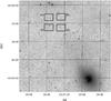 |
Fig. 1 Location and relative size of our VIMOS halo field (seen upper left), shown with respect to the center of NGC 5128/Centaurus A (lower right). The four boxes mark the regions covered by each of the four VIMOS CCDs, and lie along the major axis. The image is 70′ × 70′ and is from the STScI Digital Sky Survey. North is up and east is to the left. |
We have imaged an outer halo field of NGC 5128 in V and I bands, during ESO Periods 83 and 87 (June–July 2009, Run ID 083.B-0036A, and April–July 2011, Run ID 087.B-0135A) using service mode at the VLT. The camera was VIMOS, which has a field of view of 4 × (7′ × 8′) (i.e. 224 square arcminute), at an image scale of 0.205′′/pixel.
Our field is centered at α = 13h27m59s and δ = −42°14′50′′ (J2000.0) and lies at a projected distance of 59.9′ northeast of the galaxy’s center along the isophotal major axis (see Fig. 1). The linear projected distance to the center of our field is ≈66 kpc, or 12 Reff, where we have adopted Reff = 5.6 kpc or 305′′ (Dufour et al. 1979).
Pre-observation simulations indicated that the RGB stars would be resolved to at least a magnitude below the tip of the red-giant branch (TRGB) at ITRGB = 24.1 (Harris et al. 2010) in reasonable exposure times for seeing of 0.6 arcsec or better. In total, we obtained 8 × 705 s in I and 19 × 965 sec in V, plus one additional 88 sec exposure in V; but about half of all the acquired data were classified by ESO as “out of spec” (seeing was worse than 0.6 arcsec or had failed due to technical reasons). The four I band frames taken during Period 87 and all 20 V band frames from both periods were, despite some of which being “out of spec”, of sufficiently high quality for analysis, and were chosen to produce combined images in each band. We did not use the four I band images from Period 83 because of strong fringing. The median seeing was 0.54 arcsec and 0.68 arcsec for the I and V band frames used for analysis, respectively. The total yield in exposure times used was 47 min in I band (4 frames with FWHM = 0.5′′ combined) and 5.1 h in V (20 frames with FWHM = 0.7″ combined).
3. Data reduction and completeness
3.1. Image alignment
Pointing differences on the sky resulted in shifts between our images of up to 15 pixels. As the image plane in this wide field of view camera has significant non-linear distortions on these scales, we required 15−20 bright, isolated, unsaturated stars in each of the four quadrants of the preprocessed images supplied by ESO for image alignment. Once the 15−20 reference stars were found and matched in all exposures, the IRAF programs GEOMAP, GEOTRAN, and IMCOMBINE were used to align and combine the images. IMCOMBINE images of each quadrant were made for the two bands I and V, making a total of 8 images. The combined image was cleaned of cosmic rays, bad pixels, and other artifacts. Bad edges were present along the CCDs, and these were trimmed from the final combined frames so that all have the same size, leaving ≈70% of the field of view, or 4 ×6.9′×5.5′ (corresponding to 185 kpc2 at the source). A small segment of Quadrant 4 in the I band is shown in Fig. 2: we have marked the metal-rich and metal-poor point sources (see Sect. 5) in the field by red circles and blue squares. These point sources have magnitudes of 23.9 <I0 < 24.7 and are at least 50% complete (see Sect. 3.4).
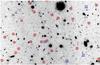 |
Fig. 2 Small ( |

3.2. Photometric calibration
Exposures of 2 s duration of Landolt standard star fields (Landolt 1992; Stetson 2000) were provided by ESO for most nights our data were taken. Typically many dozens of Landolt standards could be found in these frames, and we used these to set the photometric zeropoints of the camera in each band. The individual frames of the combined NGC 5128 image were observed at airmasses z which range from z = 1.05 to 1.19 in I and z = 1.05 to 1.42 in V and we selected standard frames taken at similar mean airmass as the NGC 5128 fields, so that uncertainties due to the airmass corrections in I and V are much less than 0.01 mag and ≈0.02 mag respectively. This is negligible compared to the dominant source of error, which is Poisson noise.
The average scatter of the standard star magnitudes, after fitting for a small color term in the zeropoint relations, was ±0.03 for I band and ±0.02 for V band, for standards with V0 > 21 (stars brighter than I0 = 21 are saturated), and we are thus confident of our zeropoints to < 0.01 mag. We calculated the average aperture correction to large radius for V and I as 0.34 and 0.19 mag, respectively, and, for the Cardelli et al. (1989) reddening law of AV/E(V − I) = 2.571 (AV/E(B − V) = 3.1), we used E(V − I) = 0.14 for the reddening and AI = 0.22 for the extinction corrections (Schlegel et al. 1998). We use the Schlegel et al. (1998) dust maps through the Galactic Dust Reddening and Extinction Service provided by NASA/IPAC Infrared Science Archive1 to estimate the variation of extinction over our field as less than 0.02 mag, negligible compared to other sources of error.
3.3. Source classification
Point sources in the field were found using two passes through the DAOPHOT II (Stetson 1992) sequence FIND/PHOT/ ALLSTAR (Stetson 1987, 1994). On average, 9 bright, isolated stars for I and 34 stars for V band were used by DAOPHOT in each quadrant with which to measure the point spread function (PSF). We used a detection threshold of 1.5 standard deviations above sky noise to produce source catalogs. After DAOPHOT located objects in both I and V bands, the two lists of objects were matched, via our own software, which pairs stars together of different bands using an initial estimate of the pixel shift between the two frames, and iterating to get the final alignment. The images reach to I0 ≈ 27.0 and V0 ≈ 28.4, or roughly three magnitudes deeper than the TRGB at I0 = 23.9 (Harris et al. 2010, we have corrected this value for extinction).
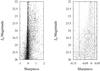 |
Fig. 3 I-band-derived sharpness parameter versus I0 band magnitudes of objects found in both I and V band combined images of VIMOS Quadrant 2 (objects detected in only one filter have been excluded). In the left panel, stars lie along the ridge of objects at the sharpness value of zero, while non-stellar or double stars lie mainly in the spread of points to the right of the ridge. Right panel: zoomed in version of the left panel. The dashed lines mark the sharpness values of −0.10 < sharpness < 0.03, in which range we have defined objects as point sources. |
We used a similar “sharpness” parameter to the one in DAOPHOT’s routine ALLSTAR to measure how point-like the sources are. Specifically, we measured the ratio of the flux in the profile of objects between 2.5 to 3.5 pixels from the center, compared to the flux in the central pixel (note well that the data are modestly oversampled, as the pixel size is 0.2 arcsec, compared to the seeing disk of 0.6 arcsec). Our sharpness parameter for an object is the difference between this ratio and the same ratio for the PSF. Sharpness values were measured for the I band images only, as they are much sharper than our V band images (the seeing was better in I, and far fewer images have been combined, to make the final I image).
In Fig. 3 (left panel) we show the distribution of the I-band-derived sharpness parameter for objects found in both the combined VIMOS (Quadrant 2) I and V band images (objects found through only one filter have been excluded). In the magnitude range 23 < I0 < 25, careful inspection by eye showed that objects with sharpness >0.05 were clearly extended (see Fig. 3), while objects <−1.0 were predominantly artifacts, such as seen around overexposed stars. We conservatively defined point sources as having −0.10 < sharpness < +0.03 in our I band image (i.e. between the dashed lines shown on the right panel of Fig. 3), after doing tests with mock stars inserted into the frames, as described in the next section. We found a total of 12 237 point sources covering a range of magnitude 21 <I0 < 27 and color −1 < (V − I)0 < 5 (see the CMDs in Figs. 7, 8).
3.4. Mock stars and sample completeness limits
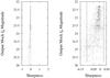 |
Fig. 4 I-band-derived sharpness versus I0 magnitudes of the mock stars recovered in both I and V filters (see also Fig. 5) as described in Sect. 3.4. Left panel: mock star sharpnesses against I0 band magnitude, and Right panel: zoomed version of the same plane. The great majority of the mock stars in the magnitude range 24 <I0 < 25 lie in the region −0.10 < sharpness < 0.03, which we use to select our point sources. |
We have estimated completeness limits for our source lists and verified our selection criteria for point sources by placing mock stars into the final aligned images in each band and re-running DAOPHOT (FIND/PHOT/ALLSTAR), to measure the recovery rate for the new sources and estimate any offset between their input and output magnitudes. We inserted 4000 mock stars into the I and V band VIMOS Quadrant 1 field, using the PSF measured for this quadrant from bright sources. The stars were assigned magnitudes randomly in the range 22 <I0 < 28 and a color of (V − I)0 = 1.2, similar to the color of the RGB stars in our field. We recovered 1571 of these mock stars, which both are matched in V and I as well as fall within our defined sharpness range for point sources of −0.10 < sharpness < 0.03. Figure 4 shows our measured sharpness parameter versus I0 band magnitude. Figure 5 shows the histograms of the injected and recovered stars as a function of apparent magnitude in 0.25 mag bins. Our recovery rate falls to 50% completeness at I0 ≈ 24.7 and V0 ≈ 25.7 (Fig. 5) and the scatter in the difference between the input and the recovered magnitudes is a satisfactory σ = ±0.1 mag in the range 24.0 <I0 < 24.7, with an offset of 0.03 mag (Fig. 6). We made a further set of three tests within Quadrant 1 using 5000 stars within a smaller range of RGB magnitudes: 24 <I0 < 25. Colors for the stars of (V − I)0 = 1.2, 1.4 and 1.7 were tested, with negligible effect on the 50% completeness limit at I0 = 24.7. We used the same 4000 artificial stars mentioned above and performed the incompleteness test with Source Extractor version 2.5 (Bertin & Arnouts 1996). The recovery rate fell to 50% completeness at I0 ≈ 24.7, in agreement with the test performed with DAOPHOT. Spatial incompleteness was not a major issue. We did tests of spatial incompleteness with mock stars added to the images with various density law falloff profiles over the CCD – and were able to recover the density profiles entirely satisfactorily. The slight photometric offsets between the four chips were small enough that experiments on one quadrant only were deemed sufficient.
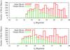 |
Fig. 5 Histograms of the number of mock stars in 0.25 mag wide bins of I0 and V0. In top panel, the solid red lined histogram includes all 4000 mock I0 band stars randomly placed in VIMOS Quadrant 1 (see lower panel for the corresponding V band histogram). The mock stars are given random I0 magnitudes in the range 22 <I0 < 28. In the top panel, the green dot dashed histogram displays the 1571 mock stars found and measured by DAOPHOT, matched with those found in the V band image, and having −0.1 < sharpness < 0.03 as measured from the I band image (see lower panel for the corresponding histogram of the 1571 objects measured in the V band image). (See the electronic edition of the journal for a color version of this figure.) |
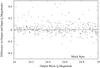 |
Fig. 6 I0 magnitudes for mock stars recovered and matched from the 4000 mock stars randomly placed within I and V band images of VIMOS Quadrant 1 (see Fig. 5 and Sect. 3.4). |
4. Foreground and background contamination and the CMD
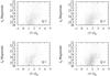 |
Fig. 7 NGC 5128 CMDs for each of the four VLT/VIMOS CCD quadrants. We count 2365, 2816, 3100, and 3956 point sources in Quadrants 1, 2, 3, and 4, respectively, within the range of magnitude 21 <I0 < 27 and color −1 < (V − I)0 < 5. Corrections have been made for the aperture size, the zeropoint dependencies on color, and the extinction. The TRGB is seen at I0 ≈ 23.9. Stars above this magnitude are predominantly from the Milky Way. Note that Quadrant 4 is the closest of the 4 quadrants to the center of NGC 5128, and has the highest source density. |
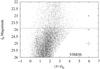 |
Fig. 8 NGC 5128 CMD for all four CCD quadrants combined. Three rectangular sections are shown, two of which are dominated by contaminants to the RGB CMD. The cleanest sample of RGB stars in the halo of NGC 5128 are found in the lower right section drawn on the CMD. Sources brighter than the TRGB at I0 = 23.9 (Harris et al. 2010, we have corrected for extinction) are field stars (upper section) – we justify this cut in Fig. 9. The lower left section (with (V − I)0 < 1.5) is dominated by unresolved background galaxies which thus appear as point sources. Justification of the choice of (V − I)0 = 1.5 for the break between background galaxy dominance and RGB dominance of the source counts can be seen in Fig. 11. Error bars for magnitude and color are indicated on the righthand side. |
CMDs of the four quadrants for the final sample of point sources found in our VIMOS field are shown in Fig. 7. We find 2365, 2816, 3100 and 3956 point sources in quadrants 1, 2, 3 and 4, respectively, for a total of 12 237 point sources covering a range of magnitude 21 <I0 < 27 and color −1 < (V − I)0 < 5. The TRGB emerges from the field stars at I0 ≈ 23.9, as observed by Harris & Harris (2000) and Harris et al. (2010), and the I band 50% completeness limit lies at I0 ≈ 24.7. Figure 8 shows all four quadrants combined into a single CMD.
Our field is located in the distant halo of NGC 5128, and in the next two subsections contamination of our source counts by foreground stars and background galaxies is carefully quantified before we isolate a clean sample of RGB stars from the halo of NGC 5128.
4.1. Foreground star contamination
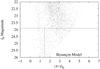 |
Fig. 9 Predictions of the Besançon model for field stars (Robin et al. 2003) in our VIMOS field. Compared to Fig. 8, the RGB window (23.9 <I0 < 24.7 and 1.5 < (V − I)0 < 3.5, as described in Sect. 4.2), is mostly uncontaminated by the Milky Way’s stars as the majority are brighter than NGC 5128’s TRGB at I0 = 23.9. Our chosen magnitude limits of I0 = 27.0 and V0 = 28.2, based on the depth of our VIMOS data, yield the diagonal cut on the righthand side of the field star predictions. |
We estimate the foreground contamination in our fields due to Milky Way stars via the Besançon field star model (Robin et al. 2003)2 using the Galactic coordinates, field of view, and depth of our VIMOS data. Figure 9 shows a CMD from the model, where we use magnitude limits of I0 = 27 and V0 = 28.2. Most (80%) of the modeled field stars lie in the magnitude range 21 <I0 < 23.9 and are brighter than the TRGB in NGC 5128 (horizontal line in the figure). Fainter than I0 = 23.9, the number of foreground stars drops rapidly, as these stars are intrinsically dim, late-type dwarfs seen at distances of the order of tens of kpc, and the number of such sources drops rapidly with apparent magnitude.
Figue 10 shows the number of foreground stars from the Besançon model (green crosses) as a function of I0 band magnitude, and is seen to be a good match to the number of point sources in our VIMOS image to I0 ≈ 23.5 (red asterisks). In this apparent magnitude range, our completeness is high. Dimmer than this, the number of foreground stars decreases to a small fraction of the total number of point sources (red asterisks).
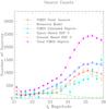 |
Fig. 10 Source counts as a function of apparent I magnitude in our VIMOS data compared to counts in the Besançon model of the Milky Way (Robin et al. 2003), space-based Hubble Deep Field South (HDF-S; Williams et al. 2000; Casertano et al. 2000), and ground-based HDF-S (da Costa et al. 1998). Both HDF-S source counts have been normalized to the field of view of VIMOS. Sources in VIMOS have been additionally subdivided into an upper limit of extended objects (blue open triangles) and point sources (red asterisks), clearly showing that an excess number of sources in our VIMOS field are detected as compared to the sources of both HDF-S fields. The predictions of the Besançon model (green crosses) are in good agreement with the number of point sources in our VIMOS field down to I0 ≈ 23.5, dimmer than which the point sources in the VIMOS field rises rapidly due to a combination of RGB stars in NGC 5128 and rising numbers of unresolved, mainly blue, background galaxies. Ground-based HDF-S (orange open squares) is a comparative example of faint background galaxy observations with similar 50% completeness at I0 = 24.6 as to our VIMOS study of I0 = 24.7. The similarity between VIMOS point source counts (red asterisks), ground-based extended source counts in the field of NGC 5128 (open blue triangles), and ground-based background galaxy counts in the field of HDS-S (open orange squares) shows that further work is needed to discriminate the two populations (cf. Sect. 4.2). Poisson error bars are added for VIMOS total sources and extended objects and for space-based and ground-based HDF-S. Incompleteness has not been corrected. Error bars for VIMOS point sources and the Besançon model are of the same scale as the plotting symbols and are not included. (See the electronic edition of the journal for a color version of this figure.) |
4.2. Background Galaxy contamination and the RGB selection window
For magnitudes dimmer than I0 ≈ 24, faint, blue galaxies become an important contributor to the source counts in our ground-based imaging, as they will be unresolved. To estimate the contamination rate of such sources in the CMD in the region of NGC 5128’s RGB, we have examined source counts in the space-based Hubble Deep Field South (HDF-S; Williams et al. 2000; Casertano et al. 2000), as these dim galaxies are well resolved from space.
We used Version 2 of the final space-based HDF-S catalog3. The catalog magnitudes were given in the AB system, the field is located high above the Galactic plane, and the detected sources go as deep as I0 = 27.4. In order to compare with our VIMOS data, we used the offsets in Table 2 of Frei & Gunn (1994) to convert the I and V band magnitudes from the AB system to the I and V used by VIMOS, namely I = I(AB) − 0.309 and V = V(AB) + 0.044. In Fig. 10, we compare the number of sources in our VIMOS image with the numbers seen in space-based HDF-S as a function of I0 band magnitude, where the space-based HDF-S counts have been scaled by a factor of 28 to match the VIMOS field of view. Dimmer than I0 = 23.5, the total number of VIMOS sources (lilac filled triangles) rises rapidly compared to space-based HDF-S (cyan filled squares), due to RGB stars in NGC 5128’s halo. These can be clearly seen down to our 50% completeness limit at I0 = 24.7 (the counts have not been corrected for completeness in this figure). Using the defined sharpness parameter of Sect. 3.3, sources in VIMOS have also been divided into extended objects (blue open triangles, 0.05 < sharpness < 1.0) and point sources (red asterisks). (Note that dimmer than I0 ≈ 25, incompleteness reduces our counts rapidly.) HDF-S gives us a means of estimating an upper limit on the number of point sources in VIMOS which are due to unresolved galaxies rather than to RGB stars in NGC 5128, and thus contaminating our counts. The comparison between our VIMOS field and HDF-S is a preliminary, quantitative comparison that will need more careful analysis in the future. As we show next, these unresolved galaxies are predominantly bluer than (V − I)0 = 1.5, and hence mainly blueward of the NGC 5128 RGB stars, such that a color cut can be used to cleanly remove them.
We show this by comparing our VIMOS data with a second field, the ground-based observations by da Costa et al. (1998) of HDF-S (Williams et al. 2000), which are represented in Fig. 10 by the open orange squares (scaled to match the total four VIMOS quadrants’ field of view, although not corrected for incompleteness). The camera used was SuSI2 (D’Odorico et al. 1998), mounted on the f/11 Nasmyth focus A of the ESO 3.58 m New Technology Telescope. The field covered 24.8 square arcminute and integrated magnitudes (corrected for reddening using Schlegel et al. 1998; E(B − V) = 0.027, yielding the extinction correction AI = 0.04 mag) were obtained using Source Extractor version 2.5 (Bertin & Arnouts 1996). da Costa et al. (1998) determined the data were 50% complete to I0 = 24.6 by comparing the region of overlap between the ground-based and space-based HDF-S catalogs, and had a stellar classification limit of I0 ≲ 22.0 (based on comparing counts from the stellar classification of Source Extractor and Milky Way model predictions). We did not make corrections for incompleteness since both VIMOS and ground-based HDF-S data share similar 50% completeness limits at I0 = 24.7 and 24.6, respectively. In the following we used the same software on our VIMOS data to facilitate as direct a comparison as possible with HDF-S, in particular to be able to compare the integrated magnitudes of the extended objects. In Fig. 11, we plot histograms by (V − I)0 color of sources in HDF-S and VIMOS Quadrant 4, in the magnitude range 23.9 <I0 < 24.7 in bins of width Δ((V − I)0) = 0.25. Note that we normalize HDF-S counts to the area of VIMOS Quadrant 4 (i.e. 36.6 square arcmin).
The first panel from the top of Fig. 11 shows the histograms by (V − I)0 color of the extended and point source objects found in VIMOS Quadrant 4 (red histogram), compared to the numbers found in ground-based HDF-S (dashed green histogram). The background galaxies in HDF-S have a color distribution which peaks at (V − I)0 ≈ 1.0, whereas the peak of the VIMOS data lies at (V − I)0 ≈ 1.8 due to the RGB stars in the field. The red histogram shows a clear excess of red sources ((V − I)0 > 1.5) due to RGB stars in NGC 5128 in the VIMOS data compared to HDF-S. In the second panel from the top, we show sources classified as resolved galaxies (extended sources) in VIMOS Quadrant 4 (red histogram), compared to the galaxies found in HDF-S (dashed green histogram). The two histograms are a fair match which indicates we are seeing the same (resolved) galaxy population in both fields. The red histogram in the third panel from the top shows all point sources from our VIMOS data. These sources consist of NGC 5128 RGB stars, unresolved background galaxies, and foreground stars. The dashed green histogram in the third panel contains the sources which remain after subtracting the two histograms from the second panel, namely the red VIMOS histogram and the dashed green HDF-S histogram of the second panel. This dashed green subtracted histogram of the third panel serves as an indicator of the color distribution of galaxies in HDF-S, which we interpret as the residual, unresolved galaxies in our VIMOS data. The two histograms of the third panel show how many of our VIMOS point sources could possibly be contaminants due to unresolved background galaxies. VIMOS point sources with V − I< 1.5 are dominated by unresolved background galaxies. In the last panel, we show two difference histograms. The red histogram gives an indication of the color distribution of sources in VIMOS Quadrant 4 interpreted as RGB stars in NGC 5128 (plus a minor contaminant of Milky Way foreground stars) and is the difference histogram produced by subtracting the red and the dashed green histograms of the first panel. The dashed green difference histogram in the last panel is the same as in the third panel. The last panel shows that redder than (V − I)0 = 1.5, contamination by unresolved galaxies in the RGB is very small (of order a few percent).
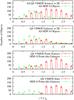 |
Fig. 11 Estimation of the unresolved galaxy contamination rate in the VIMOS data with 23.9 <I0 < 24.7 as a function of (V − I)0 color. Poisson distribution errors in number counts are shown. Incompleteness has not been corrected for either VIMOS or ground-based HDF-S. The histograms are of objects in color bins of width Δ((V − I)0 = 0.25) and are scaled to the field of view for one 36.6 square arcminute quadrant of our VIMOS data. First panel from the top: all sources from VIMOS Quadrant 4 as found by Source Extractor version 2.5 (Bertin & Arnouts 1996; red histogram) and the objects from the ground-based observations by da Costa et al. (1998) of the HST Hubble Deep Field South (HDF-S; Williams et al. 2000; dashed green histogram). Second panel from the top: extended sources in VIMOS Quadrant 4 found using Source Extractor (red histogram) and again the objects from the ground-based observations of HDF-S (dashed green histogram). Third panel from the top: the point sources from our VIMOS data as the red histogram. The dashed green histogram shows the difference between the histograms in the second panel. Last panel: two difference histograms. The red histogram shows the difference between the two histograms in the first panel. The dashed green histogram is the same as that in the third panel. See Sect. 4.2 for a full discussion of this figure. (See the electronic edition of the journal for a color version of this figure.) |
We conclude from this comparison with source counts in HDF-S, that we can reliably separate out RGB stars in NGC 5128’s halo redward of (V − I)0 = 1.5: but that blueward of this limit the counts become quickly swamped by unresolved galaxies. Hence, our final window for RGB selection is 23.9 <I0 < 24.7 and 1.5 < (V − I)0 < 3.5. We should point out that we have not made corrections for the incompleteness levels in either catalog since VIMOS and ground-based HDF-S share similar 50% completeness levels at I0 = 24.7 and 24.6, respectively. Completeness affects both the faint and the red end of the considered magnitude range (overestimating faint blue point sources due to contamination by blue, background galaxies and underestimating red sources due to the V band limit), and a more quantitative investigation of this issue will be presented in a future contribution. This is a conservative approach, as VIMOS is likely to be more affected by incompleteness than HDF-S, boosting the number of sources in the VIMOS field relative to HDF-S, and making the color cut at (V − I)0 = 1.5 more effective still in reducing the contamination of the RGB by unresolved background galaxies. The possible relaxation of such a color cut will be part of our future study.
In summary, to isolate RGB stars in NGC 5128’s outer halo, we choose the window 23.9 <I0 < 24.7 and 1.5 < (V − I)0 < 3.5 in the CMD. These selection limits are driven by the apparent magnitude of the TRGB at I0 = 23.9, the completeness limit of 50% recovered sources in both bands, at I0 = 24.7, and avoidance of predominantly blue, unresolved background galaxies (V − I)0 > 1.5. These criteria yield our final sample of 1581 point sources in our VIMOS data which we interpret as RGB stars in NGC 5128’s outer halo.
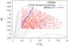 |
Fig. 12 Stellar evolutionary isochrones superimposed over the CMD for our 65 kpc field against absolute magnitude MI and (V − I)0 color. The models assume RGB stars of age 12 Gyr. Solid black lines are the α-enhanced isochrones from Pietrinferni et al. (2004, 2006); from left to right, the metallicities are [M/H] = −2.27, −1.79, −1.49, −1.27, −0.96, −0.66, −0.35, −0.25, 0.06. The dashed blue line marks [M/H]=−0.7, the cut at which we divide between metal-poor and metal-rich objects. The TRGB begins at MI = −4.05 (Rizzi et al. 2007). |
5. The metallicity and density-falloff of NGC 5128’s stellar halo
5.1. MDFs
Metallicities for our sample of RGB stars were estimated using the procedure described in Harris & Harris (2000) with the additional improvements described in Harris & Harris (2002), by interpolation of (V − I)0 colors in the BaSTI (also referred to as Teramo) 12 Gyr isochrones4 (Pietrinferni et al. 2004, 2006). We chose the α-enhanced BaSTI isochrones because the enhancement fits the old stellar halo population better than scaled-solar element ratios, as shown by Rejkuba et al. (2011) for their 40 kpc NGC 5128 field. The average α-enhancement was [ α/ Fe ] ~ 0.4, although for more details, see Pietrinferni et al. (2006) and references within. Figure 12 shows the 12 Gyr isochrones overplotted on our NGC 5128 CMD in (V − I)0 versus absolute magnitude MI, where we adopted the distance modulus of (m − M)0(TRGB) = 27.91 ± 0.08, calculated by averaging together the distance to NGC 5128 by several TRGB studies (Harris et al. 2010). Bolometric magnitudes Mbol, were estimated for the stars following Harris & Harris (2000),  where BC is the bolometric correction estimated as function of color through a rough linear two-segment curve,
  An internal uncertainty of ±0.2 in the deduced [M/H] was estimated from the combined V0 and I0 band photometric errors. For a direct comparison with the previously studied NGC 3379 halo field in which a transition in metallicity was found (Harris et al. 2007b), we adopted their metallicity cut at [M/H] = −0.7 as the division between metal-poor and metal-rich sources (dotted blue curve in Fig. 12).
We have also computed metallicities and bolometric magnitudes for stars in halo fields of NGC 5128 imaged with HST closer to the galaxy center than VIMOS, at distances of 8 kpc (Harris & Harris 2002), 21 kpc (Harris et al. 1999), 31 kpc (Harris & Harris 2000), and 40 kpc (Rejkuba et al. 2005). As these are observations from space, the background galaxies can easily be found and removed, but these galaxies are a minor component in the source counts in any case, because the surface density of RGB stars is so high compared to background galaxies, quite unlike our VIMOS field.
Raw numbers of point sources observed with HST and VLT/VIMOS, at the given projected distance (in kpc) from the center of NGC 5128, within the defined CMD overlap region 1.5 < (V − I)0 < 2.3 and −3.0 > Mbol > −3.22.
We have carefully determined over what range of color and bolometric magnitude our VIMOS study and the HST studies completely overlap in sampling of the RGB region. This turns out to be in the color range 1.5 < (V − I)0 < 2.3 and bolometric magnitude range −3.0 > Mbol > −3.22. Metallicities of the RGB stars meeting these criteria in the HST fields have been computed using the same method as we used for our 65 kpc field (namely the Teramo isochrones and the cut between metal-rich and metal-poor stars at [M/H] = −0.7). Metal-rich stars are preferentially missed because of increasing incompleteness as a function of color, although we do not correct for incompleteness in this comparison as we are especially interested in the metal-poor region. We compare the raw number counts of the metal-rich and metal-poor data within the overlap region in Table 1. While this procedure reduced our basic sample considerably, it has allowed us to examine the density falloff of both metal-rich and metal-poor stars over almost an order of magnitude in distance range, from ≈8 to ≈65 kpc.
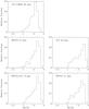 |
Fig. 13 Normalized MDFs in [M/H] for five stellar halo fields in NGC 5128, our 65 kpc VLT/VIMOS field and four HST fields: 31 kpc (Harris & Harris 2000), 40 kpc (Rejkuba et al. 2005), 8 kpc (Harris & Harris 2002), and 21 kpc (Harris et al. 1999). The data included are in the overlapping region of 1.5 < (V − I)0 < 2.3 and −3.0 > Mbol > −3.22. Neither VIMOS nor HST data has been corrected for incompleteness. |
The normalized MDF of our 65 kpc field (VIMOS) is compared with the deep HST fields of Harris & Harris (2002), Harris et al. (1999), Harris & Harris (2000), and Rejkuba et al. (2005) (8, 21, 31, and 40 kpc, respectively) in Fig. 13 over the common region of 1.5 < (V − I)0 < 2.3 and −3.0 > Mbol > −3.22. The MDFs of HST and our 65 kpc field are quite similar, indicating that our outer halo field is not obviously more metal-poor than the halo fields closer towards the center of NGC 5128. To large measure, the absence of RGB stars more metal-poor than [M/H] ≃ −1 is due to our color selection criteria (see Fig. 12), which artificially cut off almost all stars to the blue side of the [M/H] = −0.96 isochrone line. In short, we find that the predominantly metal-rich nature of the NGC 5128 halo continues on outward to at least 65 kpc or ~12 Reff.
Using data of similar quality to ours, with seeing of 0.57″−0.76″, and reaching to similar depth, Crnojević et al. (2013) found clear metal-rich and metal-poor components to the outer halo of NGC 5128. They determined metallicities for their RGB stars, finding median abundances in the range [Fe/H]med = −0.9 to −1.0, which vary little over the fields observed, despite the large range of radii covered. Taking [M/H] = [Fe/H]+[α/H] into account, their MDFs are in reasonable agreement with ours around the median abundance, given the uncertainties and different methods, but they found long tails in the MDF to low metallicity. Our color cut of (V − I)0 > 1.5 means that low metallicity stars ([M/H] ≲−1) have been explicitly removed from our sample (as they overlap in the CMD with blue, unresolved galaxies, see Fig. 12). We did not investigate the metallicity of sources in this region because we consider it to be dominated by contaminating galaxies, bluer than (V − I)0 = 1.5. Comparison with the MDFs of this paper and those of Crnojević et al. (2013) is complicated by this color cut: nevertheless, within the overlap between our RGB selection criteria (i.e. redward of (V − I)0 = 1.5), we find a fairly similar peak metallicity and negligible gradient across the field, in good agreement with the main findings of Crnojević et al. (2013).
Space-based data of these outer regions confirmed with Crnojević et al. (2013) that the MDF does reach bluer than (V − I)0 = 1.5, with blue tails more metal-poor than [M/H] = −2.0 (Rejkuba et al. 2014). The distant NGC 5128 halo regions studied by (Rejkuba et al. 2014) revealed that a gradient exists in the MDF past our 65 kpc field, although variations in metallicity exist among their fields. The average metallicity out to 140 kpc remained above [M/H] = −1.
Archival HST data for fields closer in to the center of the galaxy are available, and we intend to follow up the background contamination rates by estimating the source density of galaxies directly behind the galaxy itself, as an alternative to our comparison with the ground-based HDF-S study, as used in Sect. 4. We intend also to look at the distribution of the substantial number of stars with V − I< 1.5 found by Crnojević et al. (2013) within this future project.
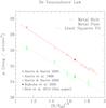 |
Fig. 14 De Vaucouleurs’ law fits (red and dashed green lines) to the surface brightness μ profile of metal-rich (red symbols with red fit line) and metal-poor (green symbols with dashed green fit line) stars in the halo of NGC 5128. We show μ in magnitudes per square arcsecond of the NGC 5128 RGB stars as a function of (R/Reff)1/4, where R is the ellipticity corrected distance from the center of the galaxy and Reff = 5.6 kpc (Dufour et al. 1979). Within this plane, μ versus (R/Reff)1/4, we use the least squares method to fit the data and solve for the slope a and y-intercept μ0 of de Vaucouleurs’ profile (de Vaucouleurs 1948) μ = a (R/Reff)1/4 + μ0, where Reff is fixed at 5.6 kpc. We correct for incompleteness by doubling the number of sources in our VIMOS field. Note that we have had to use only one distance bin for the metal-poor stars in VIMOS (due to small number statistics) whereas the metal-rich are numerous enough to be placed into 5 distance bins across the VIMOS field. Poisson distribution errors are included, although none appear for the red metal-rich symbols (fit by the red line) because the errors are of order of the same size as the symbol size. See Sect. 5.2 for a full discussion of this figure. (See the electronic edition of the journal for a color version of this figure.) |
5.2. Surface brightness profiles
In Fig. 14, we show the density falloff of metal-rich ([M/H] >−0.7) and metal-poor stars ([M/H] <−0.7) in the halo of NGC 5128, using the same overlap sample as plotted in Fig. 13, for which raw numbers are given in Table 1. To calculate the effective sampling area of our VIMOS images, we evenly spread mock sources over each quadrant and used the same DAOPHOT procedure as described in Sect. 3.3 to detect the sources. We used these detections to compute the effective sampling area on the quadrants of five radially concentric bins centered on NGC 5128. In Fig. 14, we have multiplied the VIMOS counts by a factor of two in order to account for 50% incompleteness. We also show least squares de Vaucouleurs’ law fits to the falloff luminosity μ ∝ (R/Reff)1/4 (de Vaucouleurs 1948), where μ is the surface luminosity, R is the ellipticity corrected distance from the center of the galaxy (with an ellipticity correction of b/a = 0.77, this gives corrected radii for the HST fields of 9, 24, 35, and 43 kpc), and Reff = 5.6 kpc (Dufour et al. 1979). We have converted star counts in the fields into surface brightnesses by assuming a typical apparent magnitude of I0 = 24.5 for the RGB sample since they lie in the overlap range of 24.6 > I0 > 24.35 (−3.0 > Mbol > −3.22). We fix the value of Reff to 5.6 kpc and perform a least squares fit to the data in the μ versus (R/Reff)1/4 plane. We find that the same de Vaucouleurs’ law, μ = a (R/Reff)1/4 + μ0, where a is the slope and μ0 is the y-intercept, is a good fit to both the metal-rich and metal-poor stars, with slopes of a = 7.3 ± 0.2 and 6.7 ± 0.4, respectively.
We find definite metal-rich and metal-poor halo populations, although we see no evidence of a transition from the dominating metal-rich halo to metal-poor halo in the radial falloff in density of the RGB stars in our VIMOS field and the HST fields. If the transition exists in NGC 5128, we expected the slope of the metal-rich stellar falloff to become much steeper than R1/4 near 10 Reff ≈ 60 kpc or (R/Reff)1/4 = 1.8 in Fig. 14, revealing an underlying metal-poor component, as seen in the galaxies M31 (Kalirai et al. 2006) and NGC 3379 (Harris et al. 2007b). On the contrary, the populations of both metal-rich and metal-poor stars are found out to (R/Reff)1/4 = 1.9 or 13 Reff ≈ 70 kpc and exhibit constant falling μ profiles. Any such transition must lie still further out. However, the absence of such a transition (so far) might go along with the history of NGC 5128 as a merger remnant. Age dating of the outer-halo stars in the 40 kpc field (Rejkuba et al. 2011) and of the globular clusters (Woodley et al. 2010b) consistently indicates that perhaps 1/4 of the stars were formed in some kind of merger event 3−4 Gyr ago, with the rest of the halo being classically “old” ( > 10 Gyr). A merger on this scale could dynamically shuffle the orbits well out into the halo, so even if it originally had a transition region at ~ 10 Reff as in M31 and NGC 3379, it may have been diluted or moved further outward.
Despite a significant difference between the current study and that of Crnojević et al. (2013) in the selection criteria for RGB stars, our density falloffs for halo stars are in agreement. Our selection criteria are 23.9 <I0 < 24.7 and 1.5 < (V − I)0 < 3.5, set by the magnitude of the TRGB (I0 = 23.9), our 50% completeness limit (I0 = 24.7), and the color regime in which we consider RGB stars to dominate unresolved galaxies in the source counts. Crnojević et al. (2013) used a 7-sided polygon in the CMD to select RGB stars (their Fig. 4), a procedure which differs substantially from our RGB selection in going deeper to (extinction corrected) I0 = 25.0, and extending to the blue as far as (dereddened) (V − I)0 = 1.0 (at the faint limit) and to (V − I)0 = 1.4 at the TRGB magnitude.
Crnojević et al. (2013) are well aware of potential contamination in their RGB sample, and show two profiles for the density falloff of the stellar halo in NGC 5128, based on two methods to correct for background galaxy contamination. The most conservative option is to make use of source counts in their outermost field, assuming that these are all background galaxies (at most), and subtracting these counts from fields further in. Doing this, Crnojević et al. (2013) find that the density falloff of the NGC 5128 halo can be quite well fit along the major axis by a de Vaucouleurs’ profile to 75 kpc (see their Fig. 10). We have explicitly fit a de Vaucouleurs’ profile to the Crnojević et al. (2013) stellar density falloff along the major axis (solid symbols in their Fig. 10), finding a slope of 7.1 ± 1.5, consistent with our own measure of 7.3 ± 0.2 from our combined metal-rich VIMOS and HST data and covering a much wider range of galactocentric radii. We conclude that our conservative option of cutting away sources with (V − I)0 < 1.5 to avoid background galaxy contamination, and the conservative option of Crnojević et al. (2013) of estimating background contamination from their outermost field, give a consistent picture for the density falloff of NGC 5128’s outer halo. Taking into consideration their more distant fields, Rejkuba et al. (2014) confirm that a de Vaucouleurs’ profile fits the density falloff best out to ≈56 kpc, although their more distant fields along the major axis are best fit by a power law out to 140 kpc.
6. Summary and conclusions
We have used VIMOS on VLT to image for almost 6 h in a 185 kpc2 halo field located 65 kpc (≈12 Reff) from the center of NGC 5128/Centaurus A. We obtained photometry in I and V of NGC 5128 RGB stars reliably to 0.8 mag below the TRGB at I0 = 23.9 (Harris et al. 2010).
We found that the density of RGB stars 60−70 kpc from the center of NGC 5128 is sufficiently low that contamination by unresolved background galaxies is a serious issue. By comparing with the source density of galaxies in the da Costa et al. (1998) ground-based study of Hubble Deep Field South (Williams et al. 2000), we showed that in the magnitude and color window 23.9 <I0 < 24.7 and 1.5 < (V − I)0 < 3.5, a clean sample (>99% pure) of RGB stars can be isolated. We used stellar isochrones to measure the metallicity of the stars and found a broad spread of metallicity including both a metal-rich ([M/H] >−0.7) and a metal-poor ([M/H] <−0.7) halo component, similar to what has been seen in other NGC 5128 halo fields (Harris & Harris 2002, 2000; Harris et al. 1999; Rejkuba et al. 2005), which have been observed with HST closer to the galaxy center.
We have searched for a “transition” in the metallicity distribution around 10−12 Reff from the center, in which the metal-rich component of the halo would drop away rapidly in number density relative to the metal-poor halo. This transition has been found in two morphologically different galaxies, the spiral galaxy M31 (Kalirai et al. 2006) and giant elliptical NGC 3379 (Harris et al. 2007b). We found no such transition in NGC 5128 in agreement with previous literature results based on a similar dataset, but rather see that both metal-rich and metal-poor halo stars follow the same de Vaucouleurs’ profile over radii from 8 kpc to 70 kpc. Our derived MDF and stellar density falloff are in agreement with the similar outermost halo fields of NGC 5128 studied by Crnojević et al. (2013) and Rejkuba et al. (2014).
If such a transition takes place in the halo of NGC 5128, beyond ≈75 kpc, the contamination issues of background galaxies will continue and will make it difficult to find metal-poor stars using ground-based observations of NGC 5128’s outer halo – space-based data will likely be required to work yet further out for the background galaxy separation and to probe the low metallicity tail of the MDF. NGC 5128 presents a unique field to investigate the limits of ground-based faint star detections and background galaxy contamination. We plan to exploit the extensive space- and ground-based observations of NGC 5128 to fully investigate the effects of background galaxy contamination on deep field studies of stellar populations. Such a study is especially relevant for further deep ground-based studies with the 8.2 m VLT, 10 m-class telescopes, and future telescopes such as the Thirty Meter Telescope and the 40 m European Extremely Large Telescope.
Extinction Service available at http://irsa.ipac.caltech.edu/applications/DUST/
Models available at http://model.obs-besancon.fr/
Space-based HDF-S data products available at http://www.stsci.edu/ftp/science/hdfsouth
See http://albione.oa-teramo.inaf.it/ to retrieve the evolutionary track isochrones.
Acknowledgments
S.B. thanks the Wihuri Foundation for continued funding throughout the project, the Finnish Cultural Foundation for funding the last part of the research, and the University of Turku Foundation and the StarryStory Foundation for funding travel related to the project. We are grateful for the help provided by Marina Rejkuba during the telescope application period and analysis of the 40 kpc NGC 5128 halo field, to Glen Mackie for very useful discussions, and for the care and interest taken by the referee during the reviewal process. This work has made use of BaSTI web tools.
References
- Beasley, M. A., Bridges, T., Peng, E., et al. 2008, MNRAS, 386, 1443 [NASA ADS] [CrossRef] [Google Scholar]
- Bertin, E., & Arnouts, S. 1996, A&AS, 117, 393 [NASA ADS] [CrossRef] [EDP Sciences] [Google Scholar]
- Bullock, J. S., & Johnston, K. V. 2005, ApJ, 635, 931 [NASA ADS] [CrossRef] [Google Scholar]
- Cardelli, J. A., Clayton, G. C., & Mathis, J. S. 1989, in Interstellar Dust, eds. L. J. Allamandola, & A. G. G. M. Tielens, IAU Symp., 135, 5 [Google Scholar]
- Casertano, S., de Mello, D., Dickinson, M., et al. 2000, AJ, 120, 2747 [NASA ADS] [CrossRef] [Google Scholar]
- Crnojević, D., Ferguson, A. M. N., Irwin, M. J., et al. 2013, MNRAS, 432, 832 [NASA ADS] [CrossRef] [Google Scholar]
- da Costa, L., Nonino, M., Rengelink, R., et al. 1998 [arXiv:astro-ph/9812105] [Google Scholar]
- de Vaucouleurs, G. 1948, Annales d’Astrophysique, 11, 247 [NASA ADS] [Google Scholar]
- de Vaucouleurs, G., de Vaucouleurs, A., Corwin, Jr., H. G., et al. 1991, Third Reference Catalogue of Bright Galaxies, Volume I: Explanations and references. Volume II: Data for galaxies between 0h and 12h. Volume III: Data for galaxies between 12h and 24h (Springer) [Google Scholar]
- D’Odorico, S., Beletic, J. W., Amico, P., et al. 1998, in Optical Astronomical Instrumentation, ed. S. D’Odorico, SPIE Conf. Ser., 3355, 507 [Google Scholar]
- Dufour, R. J., Harvel, C. A., Martins, D. M., et al. 1979, AJ, 84, 284 [NASA ADS] [CrossRef] [Google Scholar]
- Frei, Z., & Gunn, J. E. 1994, AJ, 108, 1476 [NASA ADS] [CrossRef] [Google Scholar]
- Graham, J. A. 1979, ApJ, 232, 60 [NASA ADS] [CrossRef] [Google Scholar]
- Gregg, M. D., Ferguson, H. C., Minniti, D., Tanvir, N., & Catchpole, R. 2004, AJ, 127, 1441 [NASA ADS] [CrossRef] [Google Scholar]
- Harris, G. L. H., & Harris, W. E. 2000, AJ, 120, 2423 [NASA ADS] [CrossRef] [Google Scholar]
- Harris, W. E., & Harris, G. L. H. 2002, AJ, 123, 3108 [NASA ADS] [CrossRef] [Google Scholar]
- Harris, G. L. H., Harris, W. E., & Poole, G. B. 1999, AJ, 117, 855 [NASA ADS] [CrossRef] [Google Scholar]
- Harris, W. E., Harris, G. L. H., Layden, A. C., & Stetson, P. B. 2007a, AJ, 134, 43 [NASA ADS] [CrossRef] [Google Scholar]
- Harris, W. E., Harris, G. L. H., Layden, A. C., & Wehner, E. M. H. 2007b, ApJ, 666, 903 [NASA ADS] [CrossRef] [Google Scholar]
- Harris, G. L. H., Rejkuba, M., & Harris, W. E. 2010, PASA, 27, 457 [NASA ADS] [CrossRef] [Google Scholar]
- Kalirai, J. S., Gilbert, K. M., Guhathakurta, P., et al. 2006, ApJ, 648, 389 [NASA ADS] [CrossRef] [Google Scholar]
- Karachentsev, I. D. 2005, AJ, 129, 178 [NASA ADS] [CrossRef] [Google Scholar]
- Landolt, A. U. 1992, AJ, 104, 340 [NASA ADS] [CrossRef] [Google Scholar]
- Malin, D. F., Quinn, P. J., & Graham, J. A. 1983, ApJ, 272, L5 [NASA ADS] [CrossRef] [Google Scholar]
- Marleau, F. R., Graham, J. R., Liu, M. C., & Charlot, S. 2000, AJ, 120, 1779 [NASA ADS] [CrossRef] [Google Scholar]
- Naab, T., Johansson, P. H., & Ostriker, J. P. 2009, ApJ, 699, L178 [NASA ADS] [CrossRef] [Google Scholar]
- Oser, L., Ostriker, J. P., Naab, T., Johansson, P. H., & Burkert, A. 2010, ApJ, 725, 2312 [NASA ADS] [CrossRef] [Google Scholar]
- Peng, E. W., Ford, H. C., Freeman, K. C., & White, R. L. 2002, AJ, 124, 3144 [NASA ADS] [CrossRef] [Google Scholar]
- Peng, E. W., Ford, H. C., & Freeman, K. C. 2004a, ApJS, 150, 367 [NASA ADS] [CrossRef] [Google Scholar]
- Peng, E. W., Ford, H. C., & Freeman, K. C. 2004b, ApJ, 602, 685 [NASA ADS] [CrossRef] [Google Scholar]
- Pietrinferni, A., Cassisi, S., Salaris, M., & Castelli, F. 2004, ApJ, 612, 168 [NASA ADS] [CrossRef] [Google Scholar]
- Pietrinferni, A., Cassisi, S., Salaris, M., & Castelli, F. 2006, ApJ, 642, 797 [NASA ADS] [CrossRef] [Google Scholar]
- Rejkuba, M., Greggio, L., Harris, W. E., Harris, G. L. H., & Peng, E. W. 2005, ApJ, 631, 262 [NASA ADS] [CrossRef] [Google Scholar]
- Rejkuba, M., Harris, W. E., Greggio, L., & Harris, G. L. H. 2011, A&A, 526, A123 [NASA ADS] [CrossRef] [EDP Sciences] [Google Scholar]
- Rejkuba, M., Harris, W. E., Greggio, L., et al. 2014, ApJ, 791, L2 [NASA ADS] [CrossRef] [Google Scholar]
- Rizzi, L., Tully, R. B., Makarov, D., et al. 2007, ApJ, 661, 815 [NASA ADS] [CrossRef] [MathSciNet] [Google Scholar]
- Robin, A. C., Reylé, C., Derriére, S., & Picaud, S. 2003, A&A, 409, 523 [NASA ADS] [CrossRef] [EDP Sciences] [Google Scholar]
- Schlegel, D. J., Finkbeiner, D. P., & Davis, M. 1998, ApJ, 500, 525 [NASA ADS] [CrossRef] [Google Scholar]
- Soria, R., Mould, J. R., Watson, A. M., et al. 1996, ApJ, 465, 79 [NASA ADS] [CrossRef] [Google Scholar]
- Stetson, P. B. 1987, PASP, 99, 191 [NASA ADS] [CrossRef] [Google Scholar]
- Stetson, P. B. 1992, in Astronomical Data Analysis Software and Systems I, eds. D. M. Worrall, C. Biemesderfer, & J. Barnes, ASP Conf. Ser., 25, 297 [Google Scholar]
- Stetson, P. B. 1994, PASP, 106, 250 [NASA ADS] [CrossRef] [Google Scholar]
- Stetson, P. B. 2000, PASP, 112, 925 [NASA ADS] [CrossRef] [Google Scholar]
- Williams, R. E., Baum, S., Bergeron, L. E., et al. 2000, AJ, 120, 2735 [NASA ADS] [CrossRef] [Google Scholar]
- Woodley, K. A., Harris, W. E., Beasley, M. A., et al. 2007, AJ, 134, 494 [NASA ADS] [CrossRef] [Google Scholar]
- Woodley, K. A., Gómez, M., Harris, W. E., Geisler, D., & Harris, G. L. H. 2010a, AJ, 139, 1871 [NASA ADS] [CrossRef] [Google Scholar]
- Woodley, K. A., Harris, W. E., Puzia, T. H., et al. 2010b, ApJ, 708, 1335 [NASA ADS] [CrossRef] [Google Scholar]
All Tables
Raw numbers of point sources observed with HST and VLT/VIMOS, at the given projected distance (in kpc) from the center of NGC 5128, within the defined CMD overlap region 1.5 < (V − I)0 < 2.3 and −3.0 > Mbol > −3.22.
All Figures
|
Fig. 1 Location and relative size of our VIMOS halo field (seen upper left), shown with respect to the center of NGC 5128/Centaurus A (lower right). The four boxes mark the regions covered by each of the four VIMOS CCDs, and lie along the major axis. The image is 70′ × 70′ and is from the STScI Digital Sky Survey. North is up and east is to the left. |
| In the text | |
|
Fig. 2 Small ( |
| In the text | |
|
Fig. 3 I-band-derived sharpness parameter versus I0 band magnitudes of objects found in both I and V band combined images of VIMOS Quadrant 2 (objects detected in only one filter have been excluded). In the left panel, stars lie along the ridge of objects at the sharpness value of zero, while non-stellar or double stars lie mainly in the spread of points to the right of the ridge. Right panel: zoomed in version of the left panel. The dashed lines mark the sharpness values of −0.10 < sharpness < 0.03, in which range we have defined objects as point sources. |
| In the text | |
|
Fig. 4 I-band-derived sharpness versus I0 magnitudes of the mock stars recovered in both I and V filters (see also Fig. 5) as described in Sect. 3.4. Left panel: mock star sharpnesses against I0 band magnitude, and Right panel: zoomed version of the same plane. The great majority of the mock stars in the magnitude range 24 <I0 < 25 lie in the region −0.10 < sharpness < 0.03, which we use to select our point sources. |
| In the text | |
|
Fig. 5 Histograms of the number of mock stars in 0.25 mag wide bins of I0 and V0. In top panel, the solid red lined histogram includes all 4000 mock I0 band stars randomly placed in VIMOS Quadrant 1 (see lower panel for the corresponding V band histogram). The mock stars are given random I0 magnitudes in the range 22 <I0 < 28. In the top panel, the green dot dashed histogram displays the 1571 mock stars found and measured by DAOPHOT, matched with those found in the V band image, and having −0.1 < sharpness < 0.03 as measured from the I band image (see lower panel for the corresponding histogram of the 1571 objects measured in the V band image). (See the electronic edition of the journal for a color version of this figure.) |
| In the text | |
|
Fig. 6 I0 magnitudes for mock stars recovered and matched from the 4000 mock stars randomly placed within I and V band images of VIMOS Quadrant 1 (see Fig. 5 and Sect. 3.4). |
| In the text | |
|
Fig. 7 NGC 5128 CMDs for each of the four VLT/VIMOS CCD quadrants. We count 2365, 2816, 3100, and 3956 point sources in Quadrants 1, 2, 3, and 4, respectively, within the range of magnitude 21 <I0 < 27 and color −1 < (V − I)0 < 5. Corrections have been made for the aperture size, the zeropoint dependencies on color, and the extinction. The TRGB is seen at I0 ≈ 23.9. Stars above this magnitude are predominantly from the Milky Way. Note that Quadrant 4 is the closest of the 4 quadrants to the center of NGC 5128, and has the highest source density. |
| In the text | |
|
Fig. 8 NGC 5128 CMD for all four CCD quadrants combined. Three rectangular sections are shown, two of which are dominated by contaminants to the RGB CMD. The cleanest sample of RGB stars in the halo of NGC 5128 are found in the lower right section drawn on the CMD. Sources brighter than the TRGB at I0 = 23.9 (Harris et al. 2010, we have corrected for extinction) are field stars (upper section) – we justify this cut in Fig. 9. The lower left section (with (V − I)0 < 1.5) is dominated by unresolved background galaxies which thus appear as point sources. Justification of the choice of (V − I)0 = 1.5 for the break between background galaxy dominance and RGB dominance of the source counts can be seen in Fig. 11. Error bars for magnitude and color are indicated on the righthand side. |
| In the text | |
|
Fig. 9 Predictions of the Besançon model for field stars (Robin et al. 2003) in our VIMOS field. Compared to Fig. 8, the RGB window (23.9 <I0 < 24.7 and 1.5 < (V − I)0 < 3.5, as described in Sect. 4.2), is mostly uncontaminated by the Milky Way’s stars as the majority are brighter than NGC 5128’s TRGB at I0 = 23.9. Our chosen magnitude limits of I0 = 27.0 and V0 = 28.2, based on the depth of our VIMOS data, yield the diagonal cut on the righthand side of the field star predictions. |
| In the text | |
|
Fig. 10 Source counts as a function of apparent I magnitude in our VIMOS data compared to counts in the Besançon model of the Milky Way (Robin et al. 2003), space-based Hubble Deep Field South (HDF-S; Williams et al. 2000; Casertano et al. 2000), and ground-based HDF-S (da Costa et al. 1998). Both HDF-S source counts have been normalized to the field of view of VIMOS. Sources in VIMOS have been additionally subdivided into an upper limit of extended objects (blue open triangles) and point sources (red asterisks), clearly showing that an excess number of sources in our VIMOS field are detected as compared to the sources of both HDF-S fields. The predictions of the Besançon model (green crosses) are in good agreement with the number of point sources in our VIMOS field down to I0 ≈ 23.5, dimmer than which the point sources in the VIMOS field rises rapidly due to a combination of RGB stars in NGC 5128 and rising numbers of unresolved, mainly blue, background galaxies. Ground-based HDF-S (orange open squares) is a comparative example of faint background galaxy observations with similar 50% completeness at I0 = 24.6 as to our VIMOS study of I0 = 24.7. The similarity between VIMOS point source counts (red asterisks), ground-based extended source counts in the field of NGC 5128 (open blue triangles), and ground-based background galaxy counts in the field of HDS-S (open orange squares) shows that further work is needed to discriminate the two populations (cf. Sect. 4.2). Poisson error bars are added for VIMOS total sources and extended objects and for space-based and ground-based HDF-S. Incompleteness has not been corrected. Error bars for VIMOS point sources and the Besançon model are of the same scale as the plotting symbols and are not included. (See the electronic edition of the journal for a color version of this figure.) |
| In the text | |
|
Fig. 11 Estimation of the unresolved galaxy contamination rate in the VIMOS data with 23.9 <I0 < 24.7 as a function of (V − I)0 color. Poisson distribution errors in number counts are shown. Incompleteness has not been corrected for either VIMOS or ground-based HDF-S. The histograms are of objects in color bins of width Δ((V − I)0 = 0.25) and are scaled to the field of view for one 36.6 square arcminute quadrant of our VIMOS data. First panel from the top: all sources from VIMOS Quadrant 4 as found by Source Extractor version 2.5 (Bertin & Arnouts 1996; red histogram) and the objects from the ground-based observations by da Costa et al. (1998) of the HST Hubble Deep Field South (HDF-S; Williams et al. 2000; dashed green histogram). Second panel from the top: extended sources in VIMOS Quadrant 4 found using Source Extractor (red histogram) and again the objects from the ground-based observations of HDF-S (dashed green histogram). Third panel from the top: the point sources from our VIMOS data as the red histogram. The dashed green histogram shows the difference between the histograms in the second panel. Last panel: two difference histograms. The red histogram shows the difference between the two histograms in the first panel. The dashed green histogram is the same as that in the third panel. See Sect. 4.2 for a full discussion of this figure. (See the electronic edition of the journal for a color version of this figure.) |
| In the text | |
|
Fig. 12 Stellar evolutionary isochrones superimposed over the CMD for our 65 kpc field against absolute magnitude MI and (V − I)0 color. The models assume RGB stars of age 12 Gyr. Solid black lines are the α-enhanced isochrones from Pietrinferni et al. (2004, 2006); from left to right, the metallicities are [M/H] = −2.27, −1.79, −1.49, −1.27, −0.96, −0.66, −0.35, −0.25, 0.06. The dashed blue line marks [M/H]=−0.7, the cut at which we divide between metal-poor and metal-rich objects. The TRGB begins at MI = −4.05 (Rizzi et al. 2007). |
| In the text | |
|
Fig. 13 Normalized MDFs in [M/H] for five stellar halo fields in NGC 5128, our 65 kpc VLT/VIMOS field and four HST fields: 31 kpc (Harris & Harris 2000), 40 kpc (Rejkuba et al. 2005), 8 kpc (Harris & Harris 2002), and 21 kpc (Harris et al. 1999). The data included are in the overlapping region of 1.5 < (V − I)0 < 2.3 and −3.0 > Mbol > −3.22. Neither VIMOS nor HST data has been corrected for incompleteness. |
| In the text | |
|
Fig. 14 De Vaucouleurs’ law fits (red and dashed green lines) to the surface brightness μ profile of metal-rich (red symbols with red fit line) and metal-poor (green symbols with dashed green fit line) stars in the halo of NGC 5128. We show μ in magnitudes per square arcsecond of the NGC 5128 RGB stars as a function of (R/Reff)1/4, where R is the ellipticity corrected distance from the center of the galaxy and Reff = 5.6 kpc (Dufour et al. 1979). Within this plane, μ versus (R/Reff)1/4, we use the least squares method to fit the data and solve for the slope a and y-intercept μ0 of de Vaucouleurs’ profile (de Vaucouleurs 1948) μ = a (R/Reff)1/4 + μ0, where Reff is fixed at 5.6 kpc. We correct for incompleteness by doubling the number of sources in our VIMOS field. Note that we have had to use only one distance bin for the metal-poor stars in VIMOS (due to small number statistics) whereas the metal-rich are numerous enough to be placed into 5 distance bins across the VIMOS field. Poisson distribution errors are included, although none appear for the red metal-rich symbols (fit by the red line) because the errors are of order of the same size as the symbol size. See Sect. 5.2 for a full discussion of this figure. (See the electronic edition of the journal for a color version of this figure.) |
| In the text | |
Current usage metrics show cumulative count of Article Views (full-text article views including HTML views, PDF and ePub downloads, according to the available data) and Abstracts Views on Vision4Press platform.
Data correspond to usage on the plateform after 2015. The current usage metrics is available 48-96 hours after online publication and is updated daily on week days.
Initial download of the metrics may take a while.