| Issue |
A&A
Volume 574, February 2015
|
|
|---|---|---|
| Article Number | A33 | |
| Number of page(s) | 14 | |
| Section | Stellar structure and evolution | |
| DOI | https://doi.org/10.1051/0004-6361/201425008 | |
| Published online | 20 January 2015 | |
Long-term variability of high-mass X-ray binaries⋆
I. Photometry
1
IESL, Foundation for Research and Technology-Hellas,
71110
Heraklion,
Greece
2
Physics Department, University of Crete,
71003
Heraklion,
Greece
e-mail:
This email address is being protected from spambots. You need JavaScript enabled to view it.
3
Observatorio Astronómico, Universidad de Valencia,
46100
Burjassot,
Spain
Received: 17 September 2014
Accepted: 7 November 2014
Abstract
We present photometric observations of the field around the optical counterparts of high-mass X-ray binaries. Our aim is to study the long-term photometric variability in correlation with their X-ray activity and derive a set of secondary standard stars that can be used for time series analysis. We find that the donors in Be/X-ray binaries exhibit larger amplitude changes in the magnitudes and colours than those hosting a supergiant companion. The amplitude of variability increases with wavelength in Be/X-ray binaries and remains fairly constant in supergiant systems. When time scales of years are considered, a good correlation between the X-ray and optical variability is observed. The X-rays cease when optical brightness decreases. These results reflect the fact that the circumstellar disk in Be/X-ray binaries is the main source of both optical and X-ray variability. We also derive the colour excess, E(B − V), selecting data at times when the contribution of the circumstellar disk was supposed to be at minimum, and we revisit the distance estimates.
Key words: techniques: photometric / stars: emission-line, Be / stars: neutron / X-rays: binaries
Finding charts with the identification of the secondary standard stars are only available at the CDS via anonymous ftp to cdsarc.u-strasbg.fr (130.79.128.5) or via http://cdsarc.u-strasbg.fr/viz-bin/qcat?J/A+A/574/A33
© ESO, 2015
1. Introduction
Neutron star high-mass X-ray binaries (HMXB) are accretion-powered binary systems where the neutron star orbits an early-type (O or B) companion. The luminosity class of the optical companion subdivides HMXBs into Be/X-ray binaries (BeXB), when the optical star is a dwarf, subgiant, or giant OBe star (luminosity class III, IV, or V), and supergiant X-ray binaries (SXRBs), if they contain an evolved star with luminosity class I–II star. In SXRBs, the optical star emits a substantial stellar wind, removing between 10-6−10-8 M⊙ yr-1 with a terminal velocity up to 2000 km s-1. A neutron star in a relatively close orbit will capture a significant fraction of this wind, sufficient to power a bright X-ray source. In BeXB, the donor is a Be star, i.e. a rapidly rotating star of spectral type early B or late O with a gaseous circumstellar envelope. In classical Be stars, the circumstellar matter is distributed in a dust-free, ionized Keplerian disk around the star’s equator (Rivinius et al. 2013). In BeXB, the main source of matter available for accretion is this circumstellar disk.
HMXBs represent important laboratories to probe physical processes in extreme conditions of gravity and magnetic fields and to study a large number of fundamental astrophysical questions, such as star formation (Grimm et al. 2003; Mineo et al. 2012), masses of neutron stars and their equation of state (van der Meer et al. 2007; Tomsick & Muterspaugh 2010; Manousakis et al. 2012), wind physics (Negueruela 2010) and particle acceleration, including supersonic and relativistic fluid dynamics, emission mechanisms, and radiation reprocessing (Hadrava & Čechura 2012; Bosch-Ramon 2013).
We have been monitoring the HMXBs visible from the northern hemisphere in the optical band since 1998. The monitoring consists of BVRI photometry and medium resolution spectra around the Hα line. Since 2013, we also obtain polarimetry in the Rc band. Here we focus on the photometry and present the results of more than ten years worth of observations. In addition to the targets, we obtained standard BVRI photometry of a large sample of stars in the HMXBs fields, from which we defined a list of secondary standard stars in the Johnson-Cousins system in each field. Secondary standards will help the monitoring of these objects in the future, as they will allow the obtention of standard photometry without the need of setting up all-sky photometric observing campaigns.
List of targets.
2. Observations
The data presented in this work were obtained from the Skinakas Observatory, located in the island of Crete (Greece). Therefore, the list of targets given in Table 1 includes HMXBs that are visible from the northern hemisphere (source declination ≳−20°). The observations cover the period 2001−2013. We analysed a total of 45 nights. The instrumental set-up consisted of the 1.3 m telescope, the Johnson-Cousins-Bessel (B, V, R, and I filters) photometric system (Bessell 1990) and a CCD camera. We employed two different CCD chips. Before 2007 June, a 1024 × 1024 SITe chip with a 24 μm pixel size (corresponding to 0.5 arcsec on the sky) was used. From 2007 July, the telescope was equipped with a 2048 × 2048 ANDOR CCD with a 13.5 μm pixel size (corresponding to 0.28 arcsec on the sky), and thus providing a field of view of ~9.5 arcmin squared.
We carried out a reduction of the data in the standard way, using the IRAF tools for aperture photometry. First, all images were bias-frame subtracted and flat-field corrected using twilight sky flats to correct for pixel-to-pixel variations on the chip. The resulting images are therefore free from the instrumental effects. We took the absorption caused by the Earth’s atmosphere into account with nightly extinction corrections determined from measurements of selected stars that also served as standards. Finally, the photometry was accurately corrected for colour equations and transformed to the standard system using nightly observations of standard stars from Landolt’s catalogue (Landolt 1992, 2009). The linear transformation equations for each filter are of the form  (1)where
  is the atmospheric-extinction-corrected instrumental magnitudes, Mj the standard value, κj is the atmospheric absorption coefficient, Xj is the airmass, tj a colour coefficient accounting for the differences in spectral response, SC is a standard star colour, and Zj is the zero point of the telescope. The subindex j runs over different filters. We used SC = (B − V) as the colour term for the B and V filters and SC = (V − R) and SC = (V − I) for the R and I filters, respectively.
We calculated the error of the photometry in the individual nights as the standard deviation of the difference between the derived final calibrated magnitudes of the standard stars and the magnitudes of the catalogue. Typically errors are of the order of 0.01–0.03 mag.
In general, all the light inside an aperture with radius equal to 16 pixels was summed up to produce the instrumental magnitudes. Because of the presence of near-by objects and larger pixel size of the older CCD, the aperture radius was reduced for XTE J1946+27 and 4U 1907+09. In the case of XTE J1946+27, the aperture radius was taken to be 10 pixels when the ANDOR CCD was used and 8 pixels in observations before 2007. For 4U 1907+09, we used 10 pixels in the observations obtained with the older CCD. We determined the sky background as the statistical mode of the counts inside an annulus 5 pixels wide and 20 pixels from the center of the object.
3. Data analysis and selection criteria for secondary standards
Although differential photometry using nearby stars has been performed on some of the targets before (Mendelson & Mazeh 1991; Bell et al. 1993; Finley et al. 1994; Goranskii 2001; Larionov et al. 2001; Baykal et al. 2005; Kızıloǧlu et al. 2007, 2009; Sarty et al. 2009), this is the first systematic attempt to define secondary standard stars within a few arcminutes of the targets that are suitable for variability studies in a large sample of sources.
The use of comparison stars, i.e. constant stars in the vicinity of the targets, permits differential photometry to be performed. Differential photometry is most suitable to investigate optical photometric variability on short (seconds to minutes) time scales. In addition, if these constant stars have well-determined magnitudes and colours in the standard system, they can be used as local standards to obtain standard photometry of the targets. This approach has a number of advantages with respect to the classical all-sky absolute photometry: it allows us to reach a higher precision; it removes the need to observe standard fields all around the sky, thus saving valuable observing time; it can be performed under less stringent weather conditions; and it eliminates the influence of instrumental drifts, since they affect every star equally.
To find constant stars in the field of view of HMXB, we first extracted the coordinates of a large number of stars using the IRAF task DAOFIND. This task searches for local density maxima, which have a given full-width half-maximum (FWHM) and a peak amplitude greater than a given threshold above the local background. Once the FWHM was fixed, we adjusted the threshold parameter to achieve at least ~40 detections in low-populated fields and ~100 in high-populated fields. Because we obtained the data using different instrumental set-up, the resulting frames differed in orientation and size, making the identification of the same star a time-consuming task. To solve this issue, we calculated the relative position of each star with respect to the target. We converted these relative positions into absolute positions in each frame by adding the coordinates of the target in that frame. Likewise, the image coordinates were scaled down in the smaller size frames (i.e. observations before 2007) by multiplying by appropriate correction factors.
Instrumental magnitudes were obtained for the target and each of the detections and then transform to the standard system. The final product was the calibrated BVRI magnitudes as a function of time. Then we derived the average and standard deviation of the data ![Mathematical equation: \begin{eqnarray} \label{mean} &&\overline{m}_{j}=\frac{\sum\limits_{i=1}^{N_j}{m_{i,j}}}{N_j} \\[1mm] \label{stdev} &&\sigma{_j}=\sqrt{\frac{\sum_{i=1}^{N_j}{(m_{i,j}-\overline{m}_j)^2}}{N_j-1}}\cdot \end{eqnarray}](/articles/aa/full_html/2015/02/aa25008-14/aa25008-14-eq66.png) The index j represents one of the four filters (BVRI) and i runs over the number of photometric measurements.The quantities Nj are the total number of good measurements in each filter. In addition, we also calculated the standard deviation of the mean as
The index j represents one of the four filters (BVRI) and i runs over the number of photometric measurements.The quantities Nj are the total number of good measurements in each filter. In addition, we also calculated the standard deviation of the mean as  (4)Secondary standard stars were selected using the following criteria:
-
Variability. Variable stars can be identified as those forwhich the standard deviation of the measured standardmagnitudes is significantly larger than the precision ofthe standard photometry on individual nights. The stan-dard deviation of the standard photometry is between 0.01and 0.03 mag for most of the ob-serving nights, as stated above. In addition, measurements ofindividual stars are also affected by instrumental photometryerrors, and by higher photon noise if the star is fainter than thestandard stars used to calculate the transformation coefficients.Taking this into account, we consider as non-variable stars thosefor which the standard deviation (Eq. (3)) of themeasurements in BVR is less or equal than 0.05 mag. Because the sky is significantly brighter in the I band, the final magnitudes resulted in slightly larger errors. Thus for the I band we allowed a larger value of 0.08 mag.
-
Number of observations. We rejected stars with fewer than six measurements.
-
Colour. The (B − V) colour index of the comparison stars brackets that of the target object. In most cases, the maximum allowed difference in (B − V) between the target and the comparison star is 0.5 mag. The only exceptions are 4U 1909+07 and EXO 2030+375, which because of the very high extinction, the comparison stars are all bluer than the target.
We imposed no limit on the magnitude of the star. Ideally, the comparison stars should be brighter than the target so that the photon noise of the target dominates that of the standards. This condition is difficult to meet if the target is bright and the field is not very populated. However, for bright objects it does not represent a problem because the secondary standards, although fainter than the target, are bright enough and are photon-noise dominated. For relatively faint targets (Vsrc≳14 mag), the selection criteria generally pick up stars that do not generally differ by more than 1 mag from the target value.
Average magnitudes and amplitude of variability of the targets.
The results of our analysis of the field stars are presented in the Appendix. We list a number of stars in the vicinity of the targets that have remained constant over year’s time scales. Thus these stars represent good secondary standard stars suitable for calibration purposes and variability studies.
4. Results on high-mass X-ray binaries
In this section we present the results of our photometric analysis of the targets. Table 2 lists the results of the observations. In this table, Col. 1 is the name of the X-ray source. Columns 2–5 contain the mean magnitudes obtained from Eq. (2). Columns 6–9 give the difference in magnitude between the maximum and minimum values. Finally, Cols. 10–13 indicate the number of observations used to derive the mean and the dispersion.
4.1. Photometric variability
Be stars are known to display photometric variability on all time scales. While rapid variability is associated with the star’s rotation and non-radial pulsations (Balona et al. 2011; Kızıloǧlu et al. 2007; Sarty et al. 2009; Gutiérrez-Soto et al. 2011), long-term variability is attributed to structural changes in the circumstellar disk. In BeXBs, the largest amplitude variations are observed on time scales of years (Lyuty & Zaĭtseva 2000; Reig et al. 2007), which represent the typical time scale for formation and dissipation of the disk (Jones et al. 2008).
Column 8 in Table 1 indicates whether the systems lost the disk during the interval covered by our observations1. By disk-loss episode, we mean that the equivalent width of the Hα line was measured positive, indicating an absorption dominated line. It is possible that a weak and small disk may be present even when emission is not detected (see e.g. Reig & Zezas 2014), but it definitively implies a low optical state.
In general, systems containing Be stars display much larger amplitude of variability in the photometric magnitudes and colours than those harbouring a supergiant companion. In the blue part of the spectrum, where ΔB ≲ 0.2 mag, SGXRBs tend to be more variable compared to ΔI< 0.1 mag. In contrast, BeXBs, especially those systems that have gone through episodes of disk dissipation and reformation, such as 4U 0115+63, 1A 0535+262, RX J0440.9+4431, and SAX J2103.5+4545 show the largest magnitude difference in the redder bands with ΔI ≫ 0.1 mag. Note however, that there are BeXBs with stable disks. These systems may show moderate changes in the individual photometric bands, but the colours hardly change on long time scales. These results are illustrated in Figs. 1 and 2. Figure 1 displays the amplitude of variability as a function of the effective wavelength for the four bandpasses considered for four BeXBs that have gone through disk-loss episodes (upper panel), four BeXB with stable disks (middle panel), four wind-fed systems, three SGXBs, and 4U 2206+54 (lower panel). These three groups of systems exhibit different behaviour. The amplitude of variability in BeXB that have gone through disk-loss episodes increases with wavelength, whereas that in wind-fed systems it decreases. The BeXB with long-lived disks show no obvious trend with wavelength. Figure 2 displays the evolution of the (B − V) colour index for three BeXB with stable disks. A linear fit to the data shows that the slope is consistent with zero. It is interesting to compare this figure with Fig. 4, where the colour index of two optically variable BeXB is shown and where large amplitude changes are apparent.
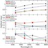 |
Fig. 1 Amplitude of magnitude change as a function of wavelength for BeXB that have gone through disk-loss episodes (upper panel), BeXB with stable disks (middle panel), and SGXB and other wind-fed systems (lower panel). |
The reason for this different behaviour is that while in BeXBs the variability comes from the disk, in supergiant stars it simply reflects the varying but relatively constant (on long time scales) mass-loss rate from the massive companion. The contribution of the disk to the overall continuum emission increases with wavelength because the slope of the thermal emission from the photosphere falls much faster than the spectral energy distribution of the free-free radiation (electron bremsstrahlung) from the disk at increasing wavelengths (Gehrz et al. 1974).
Two types of long-term correlated optical photometric and spectroscopic variations have been observed in classical Be stars (Harmanec 2000, 1983). A positive correlation is characterised by an increase in the brightness of the star as the strength of the H I lines increases. In addition, the initial brightening in the optical (e.g. V band) is accompanied by an increase in the (B − V) colour. In other words, as the disk reforms after a disk-loss phase, the systems becomes brighter and redder. On the other hand, fewer stars show a negative correlation, that is, the stronger the Hα emission, the fainter the star. In this case, the initial fading in the V band is also accompanied by a reddening of (B − V). These correlations are attributed to a geometrical effect (Harmanec 1983). Stars viewed at very high inclination angles show the inverse correlation, whereas stars seen at certain inclination angles i<icrit, exhibit the positive correlation. At very high inclination angles (equator-on stars), the inner parts of the Be envelope partly block the stellar photosphere, while the small projected area of the disk on the sky keeps the disk emission to a minimum. In stars not seen equator-on, the effect of the disk is to increase the effective radius of the star: as the disk grows an overall (star plus disk) increase in brightness is expected. The value of the critical inclination angle is not known, but a rough estimate based on available data suggest icrit ~ 75° (Sigut & Patel 2013).
Figure 3 shows four BeXB that have gone through a disk-loss phase. The Be companion in IGR J21343+4738 is the only shell star of the four (Reig & Zezas 2014). The presence of shell absorption lines indicate that the line of sight to the star lies nearly perpendicular to its rotation axis. While most of the BeXB show the positive correlation between V and (B − V), IGR J21343+4738 shows the negative correlation, hence confirming Harmanec (1983) explanation. The inverse correlation has been questioned by Haubois et al. (2012) who argued that the changes of (B − V) in shell stars should be of rather small amplitude. Large change of the (B − V) colour in this case might be due to other causes, such as V/R variations, rather than to mass injection. The current data on IGR J21343+4738 show indeed a much smaller change in (B − V) with respect to the other three sources. However, this may simply because of the fact that the disk growth is still in the initial phase in this system as indicated by the weak Hα emission (Reig & Zezas 2014).
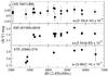 |
Fig. 2 Evolution of the (B − V) colour index in three BeXB with stable and lasting disks. s is the slope to a linear fit. |
4.2. Colour excess and distance
In Be stars, the total measured reddening is made up of two components: one produced mainly by dust in the interstellar space through the line of sight and another produced by the circumstellar gas around the Be star (Dachs et al. 1988; Fabregat & Reglero 1990). Although the physical origin and wavelength dependence of these two reddenings is completely different, their final effect upon the colours is very difficult to disentangle (Torrejón et al. 2007). Indeed, interstellar reddening is caused by “absorption” and “scattering” processes, while circumstellar reddening is due to extra “emission” at longer wavelengths. In this respect, disk-loss episodes are extremely important because they allow us to derive the true magnitudes and colours of the underlying Be star, without the contribution of the disk.
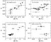 |
Fig. 3 (B − V) − V colour magnitude diagram for four BeXB that have gone through disk-loss. Note the different behaviour of IGR J21343+4738, the only BeXB with a Be shell companion. |
The colour excess is simply E(B − V) = (B − V)obs − (B − V)0, where (B − V)obs is the observed colour and (B − V)0 the intrinsic colour. To minimise the contribution of the disk, we used the data with the bluest colour index of each target. The colour excess of the sources considered in this work is listed in Table 1.
The uncertainty in estimating the distance stems from the uncertainty of the spectral classification and of the intrinsic colour and absolute magnitude calibrations. In particular, the error associated with the absolute magnitude calibration can be large (Jaschek & Gómez 1998; Wegner 2006). We estimate the intrinsic colour and absolute magnitude from the spectral type given in Table 1. The adopted (B − V)0 colour is the average of the values from Johnson (1966), Fitzgerald (1970), Gutierrez-Moreno (1979), and Wegner (1994) and the associated error, the standard deviation. The absolute magnitude was taken from Wegner (2006), who gives different calibrations for emitting and non-emitting B stars. For the error in MV, we assumed 0.5 mag. Only for the systems where the spectral type is not well constrained we took 0.6 mag. The error in the distance was then obtained by propagating the errors in V, E(B − V), (B − V)0, and MV. Typically, the error in the distance given in Table 1 is ~25%.
4.3. Correlated X-ray/optical variability
Because the disk constitutes the main reservoir of matter available for accretion, a correlation between X-rays and optical emission should be expected. Although on short time scales (days-weeks, sometimes even months) the relationship between optical emission and X-rays is complex and not always seen, when one considers time scales of years, the correlation is generally observed. The correlation identifies the circumstellar disk as the main source of optical and X-ray variability.
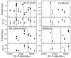 |
Fig. 4 R-band and (B − V) light curves of four BeXB displaying large amplitude X-ray activity. The dashed and dotted vertical lines indicate the epochs when type II and type I X-ray outbursts occurred, respectively. A decrease in the optical brightness following the outburst is seen in all systems. |
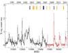 |
Fig. 5 Long-term X-ray variability of SAX J2103.5+4545 as seen by the all-sky monitors RXTE/ASM (black) and SWIFT/BAT light curves (red). The original one-day resolution light curves were rebinned to a bin size equal to the orbital period (Porb = 12.67 d). The blue and orange vertical lines indicate the epochs when the BVRI magnitudes were below (brighter) and above (fainter) the average, respectively. |
The material in the disk is the fuel that powers the X-rays through accretion. The system shines bright in X-rays while there is enough fuel. When this is exhausted the X-rays switch off. This is illustrated in Fig. 4, where a significant decline in the optical brightness is observed after the occurrence of X-ray outbursts. Figure 5 shows the long-term X-ray light curve of SAX J2103.5+4545 using the all-sky monitors on board RXTE and Swift2. The vertical blue and orange lines correspond to observations in which the photometric magnitudes were below (brighter) and above (fainter) the average, respectively (see Table 2). Clearly, low-intensity optical states are seen during faint X-ray states, whereas during bright X-ray states the source displays brighter optical magnitudes.
Sometimes the source may be active in X-rays for a very long time even after a major X-ray outburst, however, the X-rays cease once the matter supply ends. An example of this behaviour can be seen in Fig. 6, where the optical (R-band) and X-ray light curves of KS 1947+300 are shown. The X-ray data come from the all-sky monitors RXTE/ASM (2–10 keV) for observation before MJD 55 000 and from Swift/BAT (15–50 keV) after that date. During the ~five years that KS 1947+300 was active in X-rays (~MJD 51 900–53 500), the optical brightness remained fairly constant at R ~ 13.5 mag. After MJD 53 500, R decreased and the X-ray activity ceased. For the next ~eight years the optical brightness did not vary significantly (R = 13.56 ± 0.01) and the system remained in an off X-ray state. Surprisingly, the source went into another outburst without a substantial rebrightening in the optical magnitudes.
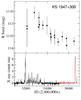 |
Fig. 6 R-band and X-ray light curves of KS 1947+300 from the RXTE/ASM (black) and Swift/BAT (red) all-sky monitors. Note the longer disk variability time-scales (changes in the optical brightness) with respect to systems shown in Fig. 4. |
Historically, the long-term X-ray variability of BeXB has been characterised by two type of outbursts.
-
Type I outbursts are regular and (quasi-)periodic outbursts, normally peaking at or close to periastron passage of the neutron star. They are short-lived, i.e. tend to cover a relatively small fraction of the orbital period (typically 0.2–0.3 Porb). The X-ray flux increases by up to two orders of magnitude with respect to the pre-outburst state, reaching peak luminosities LX ≲ 1037 erg s-1. The number of detected type I outbursts varies from source to source, but typically the source remains active for 3–8 periastron passages. A remarkable case is EXO 2030+375, which shows type I outbursts almost permanently.
-
Type II outbursts represent major increases of the X-ray flux, 103 − 104 times that at quiescence. They may reach the Eddington luminosity for a neutron star (LX ~ 1038 erg s-1) and become the brightest objects of the X-ray sky. They do not show any preferred orbital phase and last for a large fraction of an orbital period or even for several orbital periods.
Column 9 in Table 1 indicates the type of outburst detected during the course of our observation in the interval 2001–2013. It should be emphasized that as X-ray missions generate more data, it has become apparent that classification based solely on the X-ray luminosity is too simplistic. Outbursts in BeXB show a large variety of properties and many outbursts do not always follow this simple scheme (Kretschmar et al. 2012).
In principle, a type II outbursts appears as a dramatic event that may lead to the dissipation of the disk. In practice, the loss of the disk after a major outburst is the exception rather than the rule. Of the systems that exhibited type II outbursts, only 4U 0115+63 loses the disk after major outbursts (Reig et al. 2007). Nevertheless, type II outbursts do affect the structure of the disk (Fig. 4) and fainter optical emission is generally detected after such events.
Although estimating the total mass contained in a disk is rather uncertain because of the uncertainty in its size and density, an order of magnitude calculation of the amount of material that is accreted in the two cases would be illustrative. To generate an average LX ~ 1 × 1037 erg s-1 over 100 days, a mass accretion rate of Ṁ ~ 2.7 × 10¹⁷ g s-1 is needed. Assuming that all the potential energy loss in the accretion process is converted in radiation, Ṁ = LX(R/GM), then the total amount of matter accreted into the neutron star is 4.7 × 10²³ g. In the case of a type I outburst with average luminosity, LX ~ 3 × 1035 erg s-1, and a duration of 20 days, the total accreted mass would be 2.8 × 10²¹ g.
The total mass of the disk can be computed as M = ∫ρ dV, with ρ = ρ0(R∗/r)n and dV = 2πrHdr. Here ρ0 is the density and the inner radius of the disk (at r ~ R∗), R∗ the star radius, H the disk height, and n an exponent defining the density law. The parameter n varies in the range 3–3.5 in most BeX (Waters et al. 1988). The typical radius of a B0V star, is R∗ = 8 R⊙ and assuming typical values for the disk radius Rd = 5R∗, and inner density ρ0 = 10-10 g cm-3 (Telting et al. 1998) and H = 0.03R∗ (Negueruela & Okazaki 2001) the mass is estimated to be 2 × 1024 g.
Therefore, while in a type II outburst the total accreted mass may represent an important part of the disk, only an insignificant 0.1% of the total mass is accreted onto the neutron star during the course of a type I outburst. Even if the outbursts are repeated several times, the disk may not be substantially affected.
5. Summary and conclusion
We have studied the long-term optical photometric variability of the counterparts to high-mass X-ray binaries visible from the northern hemisphere. Our results can be summarised as follows:
-
1.
There is a complex connection between the optical and X-ray variability in BeXB. However, when time-scales of years are considered, there is a correlation between the long-term evolution of the system optical brightness and the X-ray activity. After a major X-ray outburst the optical magnitudes are always fainter than before the outburst.
-
2.
The disk is the main source of optical variability because the disk itself emits at these wavelength, but it is also responsible for the X-ray variability because it constitutes the source of matter available for accretion. As long as the disk is stable, no changes are seen in the colour indices. In BeXB with stable disks, the amplitude change in magnitudes shows almost no variation with wavelength.
-
3.
The more variable the BeXB in the optical band, the more variable in the X-ray band. Systems with the larger amplitude of variability in the optical magnitudes and colours are those with also the larger amplitude changes in the X-ray band.
-
4.
The HMXB with Be companions display larger amplitude of optical variability (ΔV ≫ 0.1 mag) than SGXBs (ΔV ≲ 0.1 mag).
-
5.
The amplitude of variability increases with wavelength in BeXB with fast-changing disks and decreases in SGXBs.
-
6.
The positive and negative (or inverse) correlations between luminosity and colour during disk growth observed in classical Be stars are also present in BeXBs.
-
7.
Contrary to general belief, type II outbursts do not generally lead to the total destruction of the disk, although in some cases, such as in 4U 0115+63, it does lead to the total destruction of the disk. In this system, the optical variability can be explained by a build up and disruption of the circumstellar disk on times scales of three-five years.
-
8.
We have also set up a list of secondary standard stars in the field of view of high-mass X-ray binaries. This work can benefit observers who seek to perform differential photometry for frequency analysis. It also allows us to perform standard photometry without the framework of a full all-sky absolute photometry observing campaign.
1A 0535+262 wend through a disk-loss episode in 1998 (Haigh et al. 1999).
To bring the BAT data points to the same scale as the ASM data points, we multiply the BAT data by 129.3. This constant was derived by taking into account the correspondence between intensity (mCrab) and count rate of the two instruments (1 mCrab corresponds to 0.075 ASM count s-1 and to 0.00022 BAT count cm-2 s-1) and the fact that the Crab emits about 38% more in the 2–10 keV than in the 15–50 keV band.
Acknowledgments
The work of J.F. is supported by the Spanish Ministerio de Economía y Competitividad, and FEDER, under contract AYA2010-18352. P.R. and J.F. are partially supported by the Generalitat Valenciana project of excellence PROMETEOII/2014/060. Skinakas Observatory is a collaborative project of the University of Crete and the Foundation for Research and Technology-Hellas. This work made use of NASA’s Astrophysics Data System Bibliographic Services and of the SIMBAD database, operated at the CDS, Strasbourg, France. P.R. acknowledges partial help from the COST action MP1304 “Exploring fundamental physics with compact stars”.
References
- Balona, L. A., Pigulski, A., Cat, P. D., et al. 2011, MNRAS, 413, 2403 [NASA ADS] [CrossRef] [Google Scholar]
- Baykal, A., Kızıloǧlu, Ü., Kızıloǧlu, N., Balman, Ş., & Inam, S. Ç. 2005, A&A, 439, 1131 [NASA ADS] [CrossRef] [EDP Sciences] [Google Scholar]
- Bell, S. A., Hilditch, R. W., & Pollacco, D. L. 1993, MNRAS, 265, 1042 [NASA ADS] [CrossRef] [Google Scholar]
- Bessell, M. S. 1990, PASP, 102, 1181 [NASA ADS] [CrossRef] [Google Scholar]
- Bonnarel, F., Fernique, P., Bienaymé, O., et al. 2000, A&AS, 143, 33 [NASA ADS] [CrossRef] [EDP Sciences] [Google Scholar]
- Bosch-Ramon, V. 2013, A&A, 560, A32 [NASA ADS] [CrossRef] [EDP Sciences] [Google Scholar]
- Dachs, J., Kiehling, R., & Engels, D. 1988, A&A, 194, 167 [NASA ADS] [Google Scholar]
- Fabregat, J., & Reglero, V. 1990, MNRAS, 247, 407 [NASA ADS] [Google Scholar]
- Finley, J. P., Taylor, M., & Belloni, T. 1994, ApJ, 429, 356 [NASA ADS] [CrossRef] [Google Scholar]
- Fitzgerald, M. P. 1970, A&A, 4, 234 [NASA ADS] [Google Scholar]
- Gehrz, R. D., Hackwell, J. A., & Jones, T. W. 1974, ApJ, 191, 675 [NASA ADS] [CrossRef] [Google Scholar]
- Goranskii, V. P. 2001, Astron. Lett., 27, 516 [Google Scholar]
- Grimm, H.-J., Gilfanov, M., & Sunyaev, R. 2003, MNRAS, 339, 793 [NASA ADS] [CrossRef] [Google Scholar]
- Gutierrez-Moreno, A. 1979, PASP, 91, 299 [NASA ADS] [CrossRef] [Google Scholar]
- Gutiérrez-Soto, J., Reig, P., Fabregat, J., & Fox-Machado, L. 2011, in IAU Symp., eds. C. Neiner, G. Wade, G. Meynet, & G. Peters, 272, 505 [Google Scholar]
- Hadrava, P., & Čechura, J. 2012, A&A, 542, A42 [NASA ADS] [CrossRef] [EDP Sciences] [Google Scholar]
- Haigh, N. J., Coe, M. J., Steele, I. A., & Fabregat, J. 1999, MNRAS, 310, L21 [NASA ADS] [CrossRef] [Google Scholar]
- Harmanec, P. 1983, Hvar Observatory Bulletin, 7, 55 [Google Scholar]
- Harmanec, P. 2000, in IAU Colloq. 175: The Be Phenomenon in Early-Type Stars, eds. M. A. Smith, H. F. Henrichs, & J. Fabregat, ASP Conf. Ser., 214, 13 [Google Scholar]
- Haubois, X., Carciofi, A. C., Rivinius, T., Okazaki, A. T., & Bjorkman, J. E. 2012, ApJ, 756, 156 [NASA ADS] [CrossRef] [Google Scholar]
- Jaschek, C., & Gómez, A. E. 1998, Highlights of Astronomy, 11, 566 [NASA ADS] [Google Scholar]
- Johnson, H. L. 1966, ARA&A, 4, 193 [NASA ADS] [CrossRef] [Google Scholar]
- Jones, C. E., Sigut, T. A. A., & Porter, J. M. 2008, MNRAS, 386, 1922 [NASA ADS] [CrossRef] [Google Scholar]
- Kızıloǧlu, U., Kızıloǧlu, N., Baykal, A., Yerli, S. K., & Özbey, M. 2007, A&A, 470, 1023 [NASA ADS] [CrossRef] [EDP Sciences] [Google Scholar]
- Kızıloǧlu, Ü., Özbilgen, S., Kızıloǧlu, N., & Baykal, A. 2009, A&A, 508, 895 [NASA ADS] [CrossRef] [EDP Sciences] [Google Scholar]
- Kretschmar, P., Nespoli, E., Reig, P., & Anders, F. 2012, in Proc. An INTEGRAL view of the high-energy sky (the first 10 years) 9th INTEGRAL Workshop and celebration of the 10th anniversary of the launch (INTEGRAL 2012). 15–19 October. Paris, France. Bibliotheque Nationale de France, Published online at http://pos.sissa.it/cgi-bin/reader/conf.cgi?confid=176.16 [Google Scholar]
- Landolt, A. U. 1992, AJ, 104, 340 [NASA ADS] [CrossRef] [Google Scholar]
- Landolt, A. U. 2009, AJ, 137, 4186 [NASA ADS] [CrossRef] [Google Scholar]
- Larionov, V., Lyuty, V. M., & Zaitseva, G. V. 2001, A&A, 378, 837 [NASA ADS] [CrossRef] [EDP Sciences] [Google Scholar]
- Lyuty, V. M., & Zaĭtseva, G. V. 2000, Astron. Lett., 26, 9 [Google Scholar]
- Manousakis, A., Walter, R., & Blondin, J. M. 2012, A&A, 547, A20 [NASA ADS] [CrossRef] [EDP Sciences] [Google Scholar]
- Mendelson, H., & Mazeh, T. 1991, MNRAS, 250, 373 [NASA ADS] [CrossRef] [Google Scholar]
- Mineo, S., Gilfanov, M., & Sunyaev, R. 2012, MNRAS, 419, 2095 [NASA ADS] [CrossRef] [Google Scholar]
- Negueruela, I. 2010, in High Energy Phenomena in Massive Stars, eds. J. Martí, P. L. Luque-Escamilla, & J. A. Combi, ASP. Conf. Ser., 422, 57 [Google Scholar]
- Negueruela, I., & Okazaki, A. T. 2001, A&A, 369, 108 [NASA ADS] [CrossRef] [EDP Sciences] [Google Scholar]
- Reig, P., & Zezas, A. 2014, A&A, 561, A137 [NASA ADS] [CrossRef] [EDP Sciences] [Google Scholar]
- Reig, P., Larionov, V., Negueruela, I., Arkharov, A. A., & Kudryavtseva, N. A. 2007, A&A, 462, 1081 [NASA ADS] [CrossRef] [EDP Sciences] [Google Scholar]
- Rivinius, T., Carciofi, A. C., & Martayan, C. 2013, A&ARev, 21, 69 [Google Scholar]
- Sarty, G. E., Kiss, L. L., Huziak, R., et al. 2009, MNRAS, 392, 1242 [NASA ADS] [CrossRef] [Google Scholar]
- Sigut, T. A. A., & Patel, P. 2013, ApJ, 765, 41 [NASA ADS] [CrossRef] [Google Scholar]
- Telting, J. H., Waters, L. B. F. M., Roche, P., et al. 1998, MNRAS, 296, 785 [NASA ADS] [CrossRef] [Google Scholar]
- Tomsick, J. A., & Muterspaugh, M. W. 2010, ApJ, 719, 958 [NASA ADS] [CrossRef] [Google Scholar]
- Torrejón, J. M., Negueruela, I., & Riquelme, M. S. 2007, in Active OB-Stars: Laboratories for Stellare and Circumstellar Physics, eds. A. T. Okazaki, S. P. Owocki, & S. Stefl, ASP. Conf. Ser., 361, 503 [Google Scholar]
- van der Meer, A., Kaper, L., van Kerkwijk, M. H., Heemskerk, M. H. M., & van den Heuvel, E. P. J. 2007, A&A, 473, 523 [NASA ADS] [CrossRef] [EDP Sciences] [Google Scholar]
- Waters, L. B. F. M., van den Heuvel, E. P. J., Taylor, A. R., Habets, G. M. H. J., & Persi, P. 1988, A&A, 198, 200 [NASA ADS] [Google Scholar]
- Wegner, W. 1994, MNRAS, 270, 229 [NASA ADS] [CrossRef] [Google Scholar]
- Wegner, W. 2006, MNRAS, 371, 185 [NASA ADS] [CrossRef] [Google Scholar]
Appendix A: Secondary standard stars
Table A.1 lists the final set of secondary standard stars for each target. In these tables, Col. 5 gives the angular distance between the star and the target. Columns 6–9 are the mean magnitudes, Cols. 10–13 show the standard deviation of the mean calculated from Eq. (4) and Cols. 14–17 show the number of measurements considered. The RA and Dec and the angular distance from the target to the secondary standards were derived using the ALADIN Sky Atlas (Bonnarel et al. 2000).
Finding charts with the identification of the secondary standard stars are available in electronic form at the CDS.
Secondary standards in the field of view of high-mass X-ray binaries.
All Tables
All Figures
|
Fig. 1 Amplitude of magnitude change as a function of wavelength for BeXB that have gone through disk-loss episodes (upper panel), BeXB with stable disks (middle panel), and SGXB and other wind-fed systems (lower panel). |
| In the text | |
|
Fig. 2 Evolution of the (B − V) colour index in three BeXB with stable and lasting disks. s is the slope to a linear fit. |
| In the text | |
|
Fig. 3 (B − V) − V colour magnitude diagram for four BeXB that have gone through disk-loss. Note the different behaviour of IGR J21343+4738, the only BeXB with a Be shell companion. |
| In the text | |
|
Fig. 4 R-band and (B − V) light curves of four BeXB displaying large amplitude X-ray activity. The dashed and dotted vertical lines indicate the epochs when type II and type I X-ray outbursts occurred, respectively. A decrease in the optical brightness following the outburst is seen in all systems. |
| In the text | |
|
Fig. 5 Long-term X-ray variability of SAX J2103.5+4545 as seen by the all-sky monitors RXTE/ASM (black) and SWIFT/BAT light curves (red). The original one-day resolution light curves were rebinned to a bin size equal to the orbital period (Porb = 12.67 d). The blue and orange vertical lines indicate the epochs when the BVRI magnitudes were below (brighter) and above (fainter) the average, respectively. |
| In the text | |
|
Fig. 6 R-band and X-ray light curves of KS 1947+300 from the RXTE/ASM (black) and Swift/BAT (red) all-sky monitors. Note the longer disk variability time-scales (changes in the optical brightness) with respect to systems shown in Fig. 4. |
| In the text | |
Current usage metrics show cumulative count of Article Views (full-text article views including HTML views, PDF and ePub downloads, according to the available data) and Abstracts Views on Vision4Press platform.
Data correspond to usage on the plateform after 2015. The current usage metrics is available 48-96 hours after online publication and is updated daily on week days.
Initial download of the metrics may take a while.