| Issue |
A&A
Volume 671, March 2023
|
|
|---|---|---|
| Article Number | A48 | |
| Number of page(s) | 13 | |
| Section | Stellar structure and evolution | |
| DOI | https://doi.org/10.1051/0004-6361/202245598 | |
| Published online | 03 March 2023 | |
Long-term optical variability of the Be/X-ray binary GRO J2058+42
1
Foundation for Research and Technology - Hellas, 100 Nikolaou Plastira str., Vassilika Vouton, P.O. Box 1385 70013 Heraklion, Crete, Greece
2
University of Crete, Department of Physics, Voutes University Campus, 70013 Heraklion, Greece
e-mail: This email address is being protected from spambots. You need JavaScript enabled to view it.
Received:
1
December
2022
Accepted:
17
January
2023
Abstract
Context. GRO J2058+42 is a transient hard X-ray pulsar that occasionally goes into outburst. The optical counterpart is a poorly studied OB-type companion.
Aims. We investigate the long-term optical variability of the Be/X-ray binary GRO J2058+42 and the possible connection with periods of enhanced X-ray activity.
Methods. We performed an optical spectroscopic and photometric analysis on data collected during about 18 yr. We also present the first optical polarimetric observations of this source.
Results. The long-term optical light curves in the BVRI bands and the evolution of the Hα equivalent width display a sinusoidal pattern with maxima and minima that repeat every ∼9.5 yr. The amplitude of this variability increases as the wavelength increases from 0.3 mag in the B band to 0.7 in the I band. The Hα equivalent width varied from about −0.3 to −15 Å. We found a significant decrease in the polarization degree during the low optical state. The intrinsic polarization degree changed by ∼1% from maximum to minimum. The optical maxima occur near periods of enhanced X-ray activity and are followed by a drop in the optical emission. Unlike many other Be/X-ray binaries, GRO J2058+42 does not display V/R variability.
Conclusions. The long-term optical variability agrees with the standard model of a Be/X-ray binary, where the circumstellar disk of the Be star grows and dissipates on timescales of 9−10 yr. We find that the dissipation of the disk started after a major X-ray outburst. However, the stability of the Hα line shape as a double-peak profile and the lack of asymmetries suggest the absence of a warped disk and argue against the presence of a highly distorted disk during major X-ray outbursts.
Key words: stars: neutron / stars: emission-line, Be / X-rays: binaries
© The Authors 2023
 Open Access article, published by EDP Sciences, under the terms of the Creative Commons Attribution License (https://creativecommons.org/licenses/by/4.0), which permits unrestricted use, distribution, and reproduction in any medium, provided the original work is properly cited.
This article is published in open access under the Subscribe to Open model. This email address is being protected from spambots. You need JavaScript enabled to view it. to support open access publication.
1. Introduction
GRO J2058+40 was discovered as a 198 s X-ray pulsar by BATSE on board the Compton Gamma-Ray Observatory (CGRO) during a giant outburst in 1995 September–October (Wilson et al. 1998). This giant (type II) outburst was followed by a series of weaker (type I) outbursts, whose intensity peaked at intervals of about 55 days (Wilson et al. 1998, 2005). Because BATSE detected the odd outbursts, counting from the giant outburst, to be brighter than even outbursts, it was proposed that GRO J2058+42 was undergoing periastron and apastron outburst in a 110 day orbit (Wilson et al. 1998). However, the all-sky monitor (ASM) on board the Rossi X-Ray Timing Explorer (RXTE) did not see such a pattern. Consequently, the orbital period was established to be 55 days (Wilson et al. 2005).
GRO J2058+42 was X-ray active from 1996 to 2002, but only detected at periastron passages. Pulsations were not detected during the epoch 2003−2004 (Wilson et al. 2005). GRO J2058+42 entered a new period of enhanced X-ray activity in May 2008 (Krimm et al. 2008). Although the X-ray flux doubled in less than a week, the luminosity was relatively low, LX = 1.5 × 1036 erg s−1 assuming a distance of 9 kpc (Wilson et al. 2005; Reig & Fabregat 2015). This is more consistent with the lower-luminosity type I outbursts. However, because the 2008 X-ray data were limited to just one Swift/XRT pointed observation, it is likely that the peak of the outburst was missed.
Another giant X-ray outburst occurred in March 2019 with a peak luminosity in the energy range 3−78 keV of LX = 5.6 × 1037 erg s−1 (Kabiraj & Paul 2020), similar to the discovery luminosity back in 1995. NuSTAR and AstroSat observations performed during this outburst revealed the possible presence of a cyclotron line at 10 keV together with some harmonics (Molkov et al. 2019; Mukerjee et al. 2020). During AstroSat observations, a quasi-periodic oscillation at 0.090 Hz was detected during the decay of the outburst (Mukerjee et al. 2020). The NuSTAR observations only detected the cyclotron line in a very narrow range of the spin phases of GRO J2058+42 and covering only ∼10% of the entire spin period (Molkov et al. 2019), but it did not seem to be present in the pulse-average spectrum (Kabiraj & Paul 2020).
The optical counterpart to GRO J2058+40 is an O9.5–B0e IV–V star (Reig et al. 2005; Wilson et al. 2005). The massive companion is a long-term variable system with photometric and spectroscopic changes on timescales of years (Kızıloǧlu et al. 2007; Reig & Fabregat 2015; Reig et al. 2016). The underlying B star also displays fast optical multiperiodic variability that is attributed to nonradial pulsations (Kızıloǧlu et al. 2007; Reig & Fabregat 2022). We present the most complete and detailed study of the optical variability of the BeXB GRO J2058+42 performed so far.
2. Observations and data analysis
We obtained optical photometry, spectroscopy, and polarimetry of the optical counterpart to GRO J2058+42. The observations were made from the 1.3 m telescope at the Skinakas observatory1 (SKO) in Crete (Greece). Additional spectra were retrieved from the data archive of the 2.0 m Liverpool Telescope2 (LT).
2.1. Photometry
Photometric observations with the Johnson−Cousins B, V, R, and I filters were made with the 1.3 m telescope of the Skinakas Observatory. The telescope was equipped with a 2048 × 2048 ANDOR CCD with a 13.5 μm pixel size. In this configuration, the plate scale is 0.28″/pixel, hence providing a field of view of 9.5 × 9.5 arcmin2. Standard stars from the Landolt list (Landolt 2009) were used for the transformation equations. The data were reduced in the standard way using the IRAF tools for aperture photometry3 (Tody 1986). After the standardization process, we finally assigned an error to the calibrated magnitudes of the target given by the rms of the residuals between the cataloged and calculated magnitudes of the standard stars. The photometric magnitudes are given in Table A.1.
2.2. Polarimetry
Polarimetric observations were made with the RoboPol photopolarimeter attached to the focus of the 1.3 m telescope of the Skinakas Observatory. In the polarimetry configuration a plate scale of 0.43″/pixel is achieved with a 2048 × 2048 ANDOR CCD with a 13.5 μm pixel size. RoboPol is an imaging photopolarimeter that simultaneously measures the Stokes parameters of linear polarization of all sources in the field of view (King et al. 2014; Ramaprakash et al. 2019). RoboPol splits the incident light in two beams, each half incident on a half-wave retarder followed by a Wollaston prism. The fast axis of the half-wave retarder in front of the first prism is rotated by 67.5° with respect to the other retarder. Every point in the sky is thereby projected to four points on the CCD with different polarization state. The photon counts in each spot, measured using aperture photometry, were used to calculate the U and Q parameters of linear polarization. To optimize the instrument sensitivity, a mask was placed in the telescope focal plane. The absence of moving parts allows RoboPol to compute all the Stokes parameters of linear polarization in one shot. The intrumental polarization and polarization angle zeropoint were controlled with regular measurements of polarimetric standards as described in Blinov et al. (2021). All observations were corrected for the instrumental polarization, and uncertainties were propagated accordingly. The results of the polarimetric observations are given in Table A.2.
2.3. Spectroscopy
The 1.3 m telescope at SKO was equipped with a 2048 × 2048 (13.5 micron) pixel ANDOR IKON CCD and a 1302 l mm−1 grating, giving a nominal dispersion of ∼0.9 Å/pixel. Spectra of comparison lamps were taken before and after each exposure in order to perform the wavelength calibration and account for small variations produced by the tension and flexture of the telescope at different zenith angles during the night that could affect the wavelength calibration The 2.0 m LT is a fully robotic telescope at the Roque de Los Muchachos on the Canary Island of La Palma (Spain). We downloaded and analyzed all the spectra available at the LT data archive for this source. These spectra were obtained with the Fibre-fed RObotic Dual-beam Optical Spectrograph (FRODOSpec), which is a dual-beam design multipurpose integral-field input spectrograph that splits the beam before the entrance to the individually optimized collimators. We used the spectra taken with the red arm, which cover the wavelength range 5900−8000 Å with a dispersion of 0.6 Å/pixel. A Xenon arc exposure was obtained after the science exposure. The log of the spectroscopic observations is given in Table A.4.
The Hα line is the prime indicator of the state of the disk. The structure and size of the disk affect not only the strength of the Hα line, but also its shape. We investigated the evolution of the strength and line profile over about an 18 yr period. We took the equivalent width of the Hα line (EW(Hα)) as a proxy of the strength of the line. To study the changes experienced by the shape of the line, we fit the line profile with one or two Lorentzian functions, depending on whether the line displayed a single-peak or a double-peak profile. In the case of a split profile, the peak at shorter wavelength is called the blue or violet peak, and it is denoted by V, and the peak at the longer wavelength is called the red peak and is represented by R.
The three fitting parameters are the central wavelength (λi), the full width at half maximum (FWHMi), and the relative intensity of the peak (Ii). Here the subindex i refers to either the blue (V) or red peak (R). When the line showed a double-peak profile, we obtained the following quantities: ΔV = λR − λV and V/R = log(IV/IR), where IV and IR are the intensity of the blue and red peaks relative to the continuum. For single-peak profiles, ΔV = 0 and log(V/R) was not defined.
The EW(Hα) was computed by means of a numerical integration method, the trapezoidal rule, as implemented in the scipy python package. To ensure an homogeneous processing, all the spectra were normalized with respect to the local continuum, which was rectified to unity by employing a polynomial fit. Because the definition of the continuum is the main source of uncertainty in the computation of the equivalent width, we averaged over different selections of the continuum and different polynomial fits (different grade). A total of 24 measurements were obtained for each spectrum. The error in EW(Hα) is the standard deviation of these measurements.
For the line fits, we used the deblend task of the SPLAT package (Škoda et al. 2014) of the Starklink project (Currie et al. 2014). The fits require the continuum to be at zero level. Therefore, the best polynomial fit of the continuum was subtracted from the spectra prior to the Lorentzian fits.
3. Results
3.1. Brightness variability
Figure 1 shows the long-term optical variability of GRO J2058+42. In general, the correlation among all optical observables is good. As the strength of the line emission increases, the continuum emission and the polarization increase. GRO J2058+42 went through two high and three low optical states during the course of our observations.
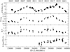 |
Fig. 1. Evolution of the optical observables. From top to bottom, we show the Hα equivalent width, continuum emission in the R band, B − V color index, and polarization degree in the R band (not corrected for ISM polarization). |
A closer look at Fig. 1 reveals some interesting results. First, the duration of the line emission in the low-optical states is significantly shorter than the continuum emission, that is, the changes in Hα occur on faster timescales than in the continuum. While the continuum emission may remain stable for years during the optical minimum, the Hα line emission reaches a minimum and begins to increase after just a few weeks. Second, the continuum emission reaches its peak by about ∼400 days before the EW(Hα) does. Third, the source exhibited stronger line and continuum emission during the 2019 high state than during the 2009 high state: EW(Hα) = −13.6 Å and R = 13.74 mag compared to EW(Hα) = −10 Å and R = 13.92 mag.
The transition from low to high states and then back to low states occurred smoothly over a period of several years. Overall, the rate of change in the EW(Hα) is roughly similar during the two transitions from the low to the high states as it is for the two declining phases. However, the changes in the optical observables during the declining phases are in general more abrupt that during the rising phases. To quantify this result, we performed a linear fit to the EW(Hα) for the four different phases, as shown in Fig. 2. The results are summarized in Table 1. The slopes of the fits are 1.5–2 times larger during the decay phase.
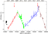 |
Fig. 2. Evolution of the Hα equivalent width. The circles represent the data, and the solid lines are the best linear fit to the data points of the corresponding interval. The red arrows mark the occurrence of an X-ray outburst. The dash style simply denotes a weaker outburst. |
Results of the linear fits to the different parts of the long-term evolution of the EW(Hα).
3.2. Hα line profile variability
In contrast to what it is typically seen in other BeXBs, the shape of the Hα line is rather symmetric. While the strength of the line changes substantially over time, as described in the previous section, the Be star in GRO J2058+42 always displays a quite symmetric double-peak profile (Fig. 3). The ratio of the peak intensities of the blue and red peaks is almost always V/R ∼ 1 (Fig. 4, bottom panel), which it is rather unusual as most BeXBs exhibit V/R variability (Reig et al. 2000, 2010; Yan et al. 2016; Alfonso-Garzón et al. 2017; Zamanov et al. 2020).
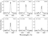 |
Fig. 3. Representative profiles of the Hα line. |
The separation between the blue and red peaks ΔV also evolves with time and is anticorrelated with EW(Hα) (Fig. 4, top panel). At the optical high states, the peak separation approaches the spectral resolution of our data (∼200 km s−1), and the two peaks merge into a single-peak profile in some spectra.
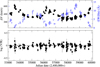 |
Fig. 4. Evolution of the Hα line parameters. Top: separation between the blue and red peaks (left axis) and the Hα EW (right axis). Bottom: evolution of the V/R ratio. |
3.3. Optical polarimetry
The continuum polarization in Be stars is attributed to Thomson scattering of unpolarized starlight in the disk (Poeckert et al. 1979; Waters & Marlborough 1992; Wood et al. 1996; Yudin 2001; Halonen et al. 2013). In general, it is difficult to compute the actual intrinsic polarization because most of the observed polarization is expected to have an interstellar origin. For example, using the relation between polarization and extinction Pmax, ISM (%) = 3.5 × E(B − V)0.8 (Fosalba et al. 2002), we estimate that the maximum contribution of the interstellar medium (ISM) to the measured optical polarization toward GRO J2058+42 is PISM = 4.6%, which is the observed polarization, on average. However, the fact that the polarization degree varies by more than 1% (from ∼4% to ∼5.2%) and that this variation correlates with EW(Hα) (it increased as the EW(Hα) increased) supports the idea that part of the observed polarization is intrinsic to the source and originates in the disk. To estimate the contribution of the ISM, we observed three nearby stars in the field of view of GRO J2058+42. Table 2 lists the field stars that we used, while Table A.3 gives the polarimetric data for these stars.
Selected field stars in the field of view of GRO J2058+42 used to derived the ISM polarization.
Figure 5 shows the change in extinction with distance and the location of the field stars and the source. The data were taken from the dust maps by Green et al. (2019). The figure indicates that at least three different molecular clouds are in between the observer and the BeXB along the line of sight. Clearly, as the distance increases, so does the polarization. The field star fs2 is too close to Earth to represent a reliable measurement of the ISM polarization at the source distance. On the other hand, gfs2 displays stronger polarization than the source, which might indicate that the star is intrinsically polarized and hence again only a poor representation of the ISM polarization. We note that at very short and long distances, the computation of the extinction is very uncertain due to the lack of sufficient number of stars. If we use fs1 to estimate the polarization from the ISM (by vector subtraction, the Q and U Stokes parameters of the source and the field star), then we obtain that the intrinsic polarization varied from 0.3% to 1.3%. The lowest value of the polarization degree corresponds to the 2013 and 2022 observations, when the EW(Hα) displayed minimum values. The level of intrinsic polarization that we measure agrees with the expected polarization in an axisymmetric circumstellar disk predicted by single-scattering plus attenuation models, which is typically ≲2% (Waters & Marlborough 1992). It also agrees with the measured polarization in a sample of classical Be stars (Yudin 2001).
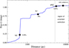 |
Fig. 5. Extinction as a function of distance (data from Green et al. 2019). The dots mark the assumed location of the stars on the extinction curve, according to their distance. Distances are from Bailer-Jones et al. (2021). We also indicate the polarization degree of each star (see Table A.3). |
3.4. Reddening and distance
Owing to the presence of the circumstellar disk, the photometric magnitudes and colors are affected by disk emission. The overall effect is to make the star appear redder, that is, to be seen under higher extinction than in the absence of the disk. As a result, the estimate of the distance obtained from photometric magnitudes that are thought to be contaminated by disk emission represents a lower limit. Some attempts have been made to quantify the contribution of the disk to the photometric indices (Dachs et al. 1988; Fabregat & Reglero 1990; Riquelme et al. 2012). Here we take advantage of the low optical states in GRO J2058+42 (Fig. 1). Because the source of long-term optical variability is the disk, low optical states correspond to instances in which the disk is almost absent. Therefore, the low optical states give us the opportunity to observe the underlying B star without a major contribution from the disk.
To estimate the distance through the distance-modulus relation, V − MV − AV = 5log(d)−5, the amount of interstellar extinction AV = R × E(B − V) to the source has to be determined. The most direct method for estimating E(B − V) is to use the calibrated color of the star according to the spectral type. The color excess is defined as E(B − V) = (B − V)obs − (B − V)0, where (B − V)obs is the observed color and (B − V)0 is the intrinsic color of the star. The expected color for an O9.5–B0V star is (B − V)0 = −0.29 ± 0.02. This value is the average of the calibrations from Johnson (1966), Fitzgerald (1970), Gutierrez-Moreno (1979), Wegner (1994), and Pecaut & Mamajek (2013). The error is the standard deviation of the five values. We applied this method to the three low optical states independently and obtained 8.6 ± 0.9 kpc, 7.8 ± 0.8 kpc, and 8.0 ± 0.9 kpc for the 2005–2006, 2012–2013, and 2022–2023 low states. We note, however, that the average Hα EW was lowest during the 2005–2006 period at EW(Hα) = −0.9 Å, compared to EW(Hα) = −3.3 Å and EW(Hα) = −1.3 Å in the other two low states, respectively. Hence we take 8.5 ± 0.8 kpc as the final value for the distance. This value compares to  kpc from Gaia (Bailer-Jones et al. 2021). The average color excess is estimated to be E(B − V) = 1.42 ± 0.02.
4. Discussion
BeXBs display variability on all timescales and at all wavelengths. The fastest variability is detected in the X-rays (on the order of seconds) and corresponds to the rotation of the neutron star, which manifests as pulsations. In the optical band, the fastest timescales (on the order of hours or days) are attributed to changes in the stellar photosphere (pulsation and rotation). Long-term variations (on the order of months to years) are related to structural changes in the disk. These long-term variations are the subject of the present work.
4.1. Disk formation and dissipation
Be star disks are known to form and dissipate on timescales of years. The disk emission increases with wavelength and becomes particularly significant in the infrared band. GRO J2058+42 went through two high (2008–2009 and 2018–2019) and three low optical states (2004–2005, 2012–2013, and 2022–2023) during the course of our observations. The transition from low to high states and then back to low states occurred smoothly over a period of several years. We attribute these long-term changes to the formation and dissipation of the circumstellar disk. As expected in the disks of Be stars, the amplitude of the variability in the continuum increases as the effective wavelength increases: the difference in magnitudes from maximum to minimum is ΔB = 0.32, ΔV = 0.46, ΔR = 0.56, and ΔI = 0.70.
4.1.1. Line and continuum emission
In Sect. 3.1 we pointed out that the line emission variability timescales are faster than the continuum emission. The BVRI magnitudes can remain at a mean value with very small fluctuations during the low optical states. For example, in the period MJD 52800–54000, the mean and standard deviation of 14 measurements of the V magnitude were 14.94 and 0.04 mag, respectively. For MJD 55800–56900 (six measurements), these values were 14.90 and 0.02 mag, respectively. In contrast, EW(Hα) does not show a stable behavior like this and varies more strongly. For the same periods, the average and standard deviation in EW(Hα) was −1.8 and −0.8 Å and −2.7 and −2.1 Å, respectively.
Another interesting result is the fact that the peak in the EW(Hα) occurred about 400 days after the peak in the photometric magnitudes. Although the observational gaps cannot be ignored, the excellent spectral coverage clearly indicates that the delay between the EW(Hα) and R-band maxima is real. These delays imply that the continuum and line emission are anticorrelated for a certain period of time (i.e., the time elapsed between the two peaks). This result has been reported in many other BeXBs: Swift J0243.6+6124 (Liu et al. 2022), RX J0440.9+4431 (Yan et al. 2016), 1A 0535+26 (Clark et al. 1999; Yan et al. 2012), 4U 0115+63 (Reig et al. 2007), and SAX J2103.5+4545 (Camero et al. 2014). Interestingly, the X-ray outbursts occur close to the EW(Hα) maxima.
This delay can be explained as due to the different locations in the disk in which the line and continuum emission in Be stars originate. The outer parts of the disk contribute most to the emission of the Hα line, whereas the origin of the optical continuum resides in the inner parts. According to the viscous decretion disk model (see Rivinius et al. 2013, for a review), about 90−95% of the V-band flux comes from inside 1.8 − 2.5 R* (Haubois et al. 2012), while Hα emission reaches this percentage above ≳6 − 10 R* (Carciofi 2011). Therefore, the fact that the optical brightness has already started to decrease by the time the EW(Hα) reached the maximum indicates that the dissipation of the disk began from the inner parts of the disk. Disk dissipation occurs when the mass ejection mechanism ceases. As the angular momentum supply stops, the inner parts of the disk are reaccreted onto the star. However, viscosity still transports angular momentum outward. Thus the outer parts of the disk continue to expand, while the inner parts move inward (Haubois et al. 2012; Carciofi et al. 2012). Since the flux in the V (or R) band is mainly produced in the inner parts of the disk, we expect the visual flux to start decreasing before the Hα line flux, which mainly originates in the outer parts.
The long-term trend of the polarization degree also supports a disk formation and dissipation cycle. Polarization in Be stars results from the scattering of stellar radiation by electrons in the circumstellar disk. The degree of the polarization provides information about the number of scatterers. Therefore, we should expect a significant decrease in the polarization degree during low optical states, as is indeed observed (Fig. 1). Since these low optical states represent instances when the disk almost vanished, we can assume that the polarization degree roughly corresponds with that of the ISM. With this assumption, we estimate that the ISM polarization from the observer to GRO J2058+42 is ∼4%.
Strictly speaking, none of the low optical states corresponded to the complete loss of the disk because the Hα line did not revert fully into absorption (see Fig. 3). A normal (i.e., non-Hα emitting) B0V star is expected to have EW(Hα) = +3.5 Å (Jaschek & Jaschek 1987), while the lowest values of EW(Hα) during the low optical states were around −[0.3 − 1] Å. Nevertheless, the low optical states do represent highly debilitated disk phases.
4.1.2. Connection with X-rays
As we mentioned above, the EW(Hα) during the 2018–2019 maximum reached higher values than during the 2008–2009 high state. Since EW(Hα) provides a measure of the size of the disk, we conclude that the Be star developed a larger disk during the 2018–2019 event. The accretion of a large amount of matter onto the neutron star led to the type II outburst observed by the NuSTAR and Astrosat space missions. In principle, it might be argued that since the disk was smaller during the 2008–2009 optical peak, the X-ray emission would be lower, as observed. On the other hand, given the similarities and regularity of the low and high optical states (Figs. 1 and 2), the absence of a giant X-ray outburst prior to the 2008–2009 optical maximum is surprising. The Swift/BAT hard X-ray transient monitor detected an increase in 15−50 keV flux by a factor of two in less than a week. A pointed observation with Swift/XRT was made on 9 May 2008. The 0.3−10 keV flux was estimated to be 1.5 × 10⁻¹⁰ erg cm−2 s−1, which at a distance of 9 kpc corresponds to a luminosity of LX = 1.4 × 1036 erg s−1 (Krimm et al. 2008). Although this luminosity is one order of magnitude lower than the 2019 event, we cannot be sure that it corresponded to the peak of the X-ray event. The 2008–2009 is reminiscent of a type I outburst, and the lack of data can be attributed to the weakness of the detection due to the large distance to the source.
One possible explanation for the different luminosity of the two events could be a different geometry in a misaligned and tilted disk. Current models that explain X-ray outbursts in BeXBs invoke warped, tilted, and misaligned disks. Because disks in BeXBs are truncated (Reig et al. 1997, 2016), the only way for large amount of material to be transferred to the neutron star is in highly asymmetric configurations in which a misaligned disk becomes warped and eccentric. Highly distorted disks result in enhanced mass accretion when the neutron star moves across the warped part (Martin et al. 2011, 2014; Okazaki et al. 2013). Evidence of these warped disks has been reported for 1A 0535+262 (Moritani et al. 2013) based on a spectral line analysis and for 4U 0115 (Reig & Blinov 2018) based on variations in the polarization angle. Although we observe a small change in the polarization angle during the 2019 X-ray outburst (Fig. 6), it is not very significant. Likewise, the symmetry of the Hα line profile argues against a highly distorted disk. Therefore, it remains to be seen how a type I outburst can lead to the almost complete destruction of the circumstellar disk.
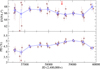 |
Fig. 6. Polarization angle and polarization degree of GRO J2058+42 for the period 2013–2022. The red arrow marks the occurrence of a type II outburst. Filled brown circles denote all the observations, and the open blue circles represent the weighted mean calculated using the observations over one year. |
We also noted in Sect. 3.1 that the dissipation of the disk is faster than its formation. The rate of change of the Hα equivalent width is about 1.8 Å yr−1 during disk formation and about 3.3 Å yr−1 during disk dissipation (see Fig. 2 and Table 1). This result contrasts with what it is observed in classical Be stars, in which the timescales for disk growth are shorter than the timescales for disk dissipation (Haubois et al. 2012). A crucial difference is the presence of the neutron star in BeXBs. As the disk expands and reaches periastron distance, a substantial amount of matter will be accreted onto the neutron star. Therefore, the dissipation of the disk in BeXBs may occur faster owing to the interaction between the neutron star and the disk.
4.2. Inclination angle
We showed in Sect. 3.2 that the source displays a double-peak profile even during the high optical state (see Fig. 3). This result suggests that we see the circumstellar disk at an intermediate inclination angle. Typically, single-peak profiles are associated with high inclination angles (pole-on stars) and shell profiles with high inclination angles (edge-on stars; Slettebak 1979; Hanuschik 1995; Rivinius et al. 2006; Silaj et al. 2014; Sigut & Ghafourian 2022). An example of a low inclination system is V 0332+54, whose inclination angle is estimated to be i < 20° (Negueruela et al. 1999; Zhang et al. 2005), and a BeXB that exhibits shell profiles is IGR J21343+4738 (Reig & Zezas 2014).
The evolution of the photometric magnitudes and colors can also be used to constrain the inclination angle. Figure 7 shows the color-magnitude diagram of GRO J2058+42. Empty symbols correspond to the disk formation phases, and filled symbols correspond to the dissipation phases. The positive correlation between the color index (B − V) and the V magnitude implies that the system is viewed at an intermediate inclination angle, where the disk emission to the optical colors and magnitudes contributes significantly. As the disk grows, the system brightens (V decreases), while the overall (disk plus star) emission becomes redder ((B − V) increases). At very high inclination angles (equator-on stars), the inner parts of the Be envelope partly block the stellar photosphere, while the small projected area of the disk on the sky keeps the disk emission to a minimum. Thus, stars viewed at very high inclination angles (i > icrit) would show an inverse correlation (Harmanec 1983; Harmanec et al. 2000). The value of the critical inclination angle is not known, but a rough estimate based on available data suggests icrit ∼ 60 − 70° (Hanuschik 1996; Sigut & Patel 2013). In summary, the correlation between the photometric colors and magnitudes and the stable double peak profile of the Hα line in GRO J2058+42 suggest an inclination angle in the range 30° −60°.
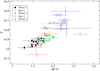 |
Fig. 7. (B − V)−V color magnitude diagram. Empty symbols correspond to the disk formation phases, and filled symbols correspond to the dissipation phases. |
4.3. Disk size and kinematics
It was already proposed by Struve (1931) that disks in Be stars are supported by rotation. The main evidence for this comes from the correlation between the projected rotational velocity and the width and shape of the emission line (Andrillat 1983; Dachs et al. 1986, 1992; Hanuschik et al. 1988; Hanuschik 1989).
In Sect. 3.2 we showed that the peak separation ΔV and EW(Hα) are anticorrelated. This is the expected behavior in rotation-supported disks, in which the rotational velocity of the gas particles in the disk varies as the inverse of the radius, vϕ ∝ r−j (e.g., for Keplerian disks j = 1/2). In these disks, the peak separation roughly corresponds to twice the projected rotational velocity of the particles in the disk ΔV ≈ 2vϕ sin i. As the radius of the disk increases (i.e., as EW(Hα) increases), the rotational velocity decreases, and so does the peak separation. The index j can be estimated from the relation between peak separation and EW (Hanuschik et al. 1988),
 (1)
(1)
where the slope a is related to the j index as a = j/2. Figure 8 shows this relation for GRO J2058+42. When we restrict the fitting range to EWs between 1 and 8 Å, then we find j = 0.58 ± 0.04, which is not far from the expected value of 0.5 for a Keplerian disk. Lower and higher values of the EW(Hα) were removed from the fit because below log(EW(Hα)) ∼ 0 the disk is too small and has probably not reached a stable configuration, while above 8 Å, the ΔV saturates, which might be a spectral resolution effect.
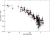 |
Fig. 8. Peak separation as a function of EW(Hα). |
After showing that the particles in the disk of GRO J2058+42 follow a Keplerian law, we can estimate the disk size. The disk velocity adopts the form (see. e.g., Huang 1972)
 (2)
(2)
where R* is the equatorial stellar radius, and v0 is a initial value of the disk velocity close to the stellar surface. In the limiting case, v0 would be the stellar rotational velocity. For simplicity, we assumed v0 = v*. By inverting Eq. (2) and since vϕ ≈ (ΔV/2 sin i),
 (3)
(3)
where r = Rd is the radius of the Hα emission region. Figure 9 shows the size of the circumstellar disk as a function of time and EW(Hα). As mentioned above, the leveling off at ∼50 R⊙ marks the minimum distance between the peaks that our spectrograph is capable of discerning.
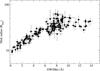 |
Fig. 9. Disk radius as a function of EW(Hα). |
The Be star projected rotational velocity in GRO J2058+42 has been estimated by Kızıloǧlu et al. (2007) to be in the range 240−310 km s−1. Here we assumed v* sin i = 275 km s−1, which corresponds to half the maximum peak separation. We note, however, that Hα double-peak separation exceeding 2v* sin i has been measured in Be stars during phases of very weak Hα emission (Dachs et al. 1992).
The largest disk radius is estimated to be Rdisk, max ∼ 5 − 6 R* or 60 R⊙, assuming a stellar radius of an O9.5–B0e IV–V star of 10 R⊙ (Martins et al. 2005). From Kepler’s third law, we can estimate the orbital separation a ∼ 160 R⊙ for Porb = 55 days and typical values of the mass M* = 18 M⊙. If we now assume that in order to produce an X-ray outburst, the neutron star must interact with the disk, that is, the disk radius must be similar to the periastron distance (a(1 − e)), then the eccentricity of the system should be e ∼ 0.6.
5. Conclusion
We have performed the most detailed study of the long-term optical variability of the BeXB GRO J2058+42. The system displays correlated variability on timescales of years in all the optical observables. The source goes through optical high and low states. The high optical state is characterized by large EW(Hα), bright continuum emission, and significant polarization. We identify this state with a well-developed decretion disk. The smooth increases and decreases of the optical emission are interpreted as phases of formation and dissipation of the circumstellar disk. The optical maxima coincide with the occurrence of X-ray outbursts, after which all optical indicators decreased, leading to the dissipation of the disk. However, a disk-loss episode never occurred. The almost permanent double-peak line profile indicates that the systems is seen at an intermediate inclination angle, whereas the absence of V/R variability is attributed to a relatively small and stable disk. We did not find evidence for a warped disk during the 2019 type II X-ray outburst.
A User’s Guide to CCD Reductions with IRAF, Philip Massey, February 1997. https://iraf.net/irafdocs
Acknowledgments
Skinakas Observatory is run by the University of Crete and the Foundation for Research and Technology-Hellas. The Liverpool Telescope is owned and operated by the Astrophysics Research Institute of Liverpool John Moores University. The Starlink software is currently supported by the East Asian Observatory. IRAF is distributed by the National Optical Astronomy Observatories, which is operated by the Association of Universities for Research in Astronomy, Inc. (AURA) under cooperative agreement with the National Science Foundation. This research has made use of the SIMBAD database, operated at CDS, Strasbourg, France and of NASA’s Astrophysics Data System operated by the Smithsonian Astrophysical Observatory.
References
- Alfonso-Garzón, J., Fabregat, J., Reig, P., et al. 2017, A&A, 607, A52 [NASA ADS] [CrossRef] [EDP Sciences] [Google Scholar]
- Andrillat, Y. 1983, A&AS, 53, 319 [NASA ADS] [Google Scholar]
- Bailer-Jones, C. A. L., Rybizki, J., Fouesneau, M., Demleitner, M., & Andrae, R. 2021, AJ, 161, 147 [Google Scholar]
- Blinov, D., Kiehlmann, S., Pavlidou, V., et al. 2021, MNRAS, 501, 3715 [NASA ADS] [CrossRef] [Google Scholar]
- Camero, A., Zurita, C., Gutiérrez-Soto, J., et al. 2014, A&A, 568, A115 [NASA ADS] [CrossRef] [EDP Sciences] [Google Scholar]
- Carciofi, A. C. 2011, in IAU Symposium, eds. C. Neiner, G. Wade, G. Meynet, & G. Peters, 272, 325 [NASA ADS] [Google Scholar]
- Carciofi, A. C., Bjorkman, J. E., Otero, S. A., et al. 2012, ApJ, 744, L15 [Google Scholar]
- Clark, J. S., Lyuty, V. M., Zaitseva, G. V., et al. 1999, MNRAS, 302, 167 [NASA ADS] [CrossRef] [Google Scholar]
- Currie, M. J., Berry, D. S., Jenness, T., et al. 2014, in Astronomical Data Analysis Software and Systems XXIII, ed. N. Manset, ASP Conf. Ser., 485, 391 [NASA ADS] [Google Scholar]
- Dachs, J., Hanuschik, R., Kaiser, D., & Rohe, D. 1986, A&A, 159, 276 [NASA ADS] [Google Scholar]
- Dachs, J., Kiehling, R., & Engels, D. 1988, A&A, 194, 167 [NASA ADS] [Google Scholar]
- Dachs, J., Hummel, W., & Hanuschik, R. W. 1992, A&AS, 95, 437 [NASA ADS] [Google Scholar]
- Fabregat, J., & Reglero, V. 1990, MNRAS, 247, 407 [NASA ADS] [Google Scholar]
- Fitzgerald, M. P. 1970, A&A, 4, 234 [NASA ADS] [Google Scholar]
- Fosalba, P., Lazarian, A., Prunet, S., & Tauber, J. A. 2002, ApJ, 564, 762 [NASA ADS] [CrossRef] [Google Scholar]
- Green, G. M., Schlafly, E., Zucker, C., Speagle, J. S., & Finkbeiner, D. 2019, ApJ, 887, 93 [NASA ADS] [CrossRef] [Google Scholar]
- Gutierrez-Moreno, A. 1979, PASP, 91, 299 [NASA ADS] [CrossRef] [Google Scholar]
- Halonen, R. J., Mackay, F. E., & Jones, C. E. 2013, ApJS, 204, 11 [NASA ADS] [CrossRef] [Google Scholar]
- Hanuschik, R. W. 1989, Ap&SS, 161, 61 [NASA ADS] [CrossRef] [Google Scholar]
- Hanuschik, R. W. 1995, A&A, 295, 423 [NASA ADS] [Google Scholar]
- Hanuschik, R. W. 1996, A&A, 308, 170 [NASA ADS] [Google Scholar]
- Hanuschik, R. W., Kozok, J. R., & Kaiser, D. 1988, A&A, 189, 147 [NASA ADS] [Google Scholar]
- Harmanec, P. 1983, Hvar Obs. Bull., 7, 55 [NASA ADS] [Google Scholar]
- Harmanec, P. 2000, in IAU Colloq. 175: The Be Phenomenon in Early-Type Stars, eds. M. A. Smith, H. F. Henrichs, & J. Fabregat, ASP Conf. Ser., 214, 13 [NASA ADS] [Google Scholar]
- Haubois, X., Carciofi, A. C., Rivinius, T., Okazaki, A. T., & Bjorkman, J. E. 2012, ApJ, 756, 156 [Google Scholar]
- Huang, S.-S. 1972, ApJ, 171, 549 [NASA ADS] [CrossRef] [Google Scholar]
- Jaschek, C., & Jaschek, M. 1987, The Classification of Stars (Cambridge: Cambridge University Press) [Google Scholar]
- Johnson, H. L. 1966, ARA&A, 4, 193 [NASA ADS] [CrossRef] [Google Scholar]
- Kabiraj, S., & Paul, B. 2020, MNRAS, 497, 1059 [NASA ADS] [CrossRef] [Google Scholar]
- King, O. G., Blinov, D., Ramaprakash, A. N., et al. 2014, MNRAS, 442, 1706 [NASA ADS] [CrossRef] [Google Scholar]
- Kızıloǧlu, U., Kızıloǧlu, N., Baykal, A., Yerli, S. K., & Özbey, M. 2007, A&A, 470, [Google Scholar]
- Krimm, H. A., Barthelmy, S. D., Baumgartner, W., et al. 2008, ATel, 1516, 1 [NASA ADS] [Google Scholar]
- Landolt, A. U. 2009, AJ, 137, 4186 [Google Scholar]
- Liu, W., Yan, J., Reig, P., et al. 2022, A&A, 666, A110 [NASA ADS] [CrossRef] [EDP Sciences] [Google Scholar]
- Martin, R. G., Pringle, J. E., Tout, C. A., & Lubow, S. H. 2011, MNRAS, 416, 2827 [NASA ADS] [CrossRef] [Google Scholar]
- Martin, R. G., Nixon, C., Armitage, P. J., Lubow, S. H., & Price, D. J. 2014, ApJ, 790, L34 [Google Scholar]
- Martins, F., Schaerer, D., & Hillier, D. J. 2005, A&A, 436, 1049 [NASA ADS] [CrossRef] [EDP Sciences] [Google Scholar]
- Molkov, S., Lutovinov, A., Tsygankov, S., Mereminskiy, I., & Mushtukov, A. 2019, ApJ, 883, L11 [NASA ADS] [CrossRef] [Google Scholar]
- Moritani, Y., Nogami, D., Okazaki, A. T., et al. 2013, PASJ, 65, 83 [NASA ADS] [Google Scholar]
- Mukerjee, K., Antia, H. M., & Katoch, T. 2020, ApJ, 897, 73 [NASA ADS] [CrossRef] [Google Scholar]
- Negueruela, I., Roche, P., Fabregat, J., & Coe, M. J. 1999, MNRAS, 307, 695 [NASA ADS] [CrossRef] [Google Scholar]
- Okazaki, A. T., Hayasaki, K., & Moritani, Y. 2013, PASJ, 65, 41 [NASA ADS] [Google Scholar]
- Pecaut, M. J., & Mamajek, E. E. 2013, ApJS, 208, 9 [Google Scholar]
- Poeckert, R., Bastien, P., & Landstreet, J. D. 1979, AJ, 84, 812 [NASA ADS] [CrossRef] [Google Scholar]
- Ramaprakash, A. N., Rajarshi, C. V., Das, H. K., et al. 2019, MNRAS, 485, 2355 [NASA ADS] [CrossRef] [Google Scholar]
- Reig, P., & Blinov, D. 2018, A&A, 619, A19 [NASA ADS] [CrossRef] [EDP Sciences] [Google Scholar]
- Reig, P., & Fabregat, J. 2015, A&A, 574, A33 [NASA ADS] [CrossRef] [EDP Sciences] [Google Scholar]
- Reig, P., & Fabregat, J. 2022, A&A, 667, A18 [NASA ADS] [CrossRef] [EDP Sciences] [Google Scholar]
- Reig, P., & Zezas, A. 2014, A&A, 561, A137 [NASA ADS] [CrossRef] [EDP Sciences] [Google Scholar]
- Reig, P., Fabregat, J., & Coe, M. J. 1997, A&A, 322, 193 [NASA ADS] [Google Scholar]
- Reig, P., Negueruela, I., Coe, M. J., et al. 2000, MNRAS, 317, 205 [NASA ADS] [CrossRef] [Google Scholar]
- Reig, P., Negueruela, I., Papamastorakis, G., Manousakis, A., & Kougentakis, T. 2005, A&A, 440, 637 [NASA ADS] [CrossRef] [EDP Sciences] [Google Scholar]
- Reig, P., Larionov, V., Negueruela, I., Arkharov, A. A., & Kudryavtseva, N. A. 2007, A&A, 462, 1081 [NASA ADS] [CrossRef] [EDP Sciences] [Google Scholar]
- Reig, P., Zezas, A., & Gkouvelis, L. 2010, A&A, 522, A107 [NASA ADS] [CrossRef] [EDP Sciences] [Google Scholar]
- Reig, P., Nersesian, A., Zezas, A., Gkouvelis, L., & Coe, M. J. 2016, A&A, 590, A122 [NASA ADS] [CrossRef] [EDP Sciences] [Google Scholar]
- Riquelme, M. S., Torrejón, J. M., & Negueruela, I. 2012, A&A, 539, A114 [NASA ADS] [CrossRef] [EDP Sciences] [Google Scholar]
- Rivinius, T., Štefl, S., & Baade, D. 2006, A&A, 459, 137 [NASA ADS] [CrossRef] [EDP Sciences] [Google Scholar]
- Rivinius, T., Carciofi, A. C., & Martayan, C. 2013, A&ARv, 21, 69 [Google Scholar]
- Sigut, T. A. A., & Ghafourian, N. R. 2022, arXiv e-prints [arXiv:2209.06885] [Google Scholar]
- Sigut, T. A. A., & Patel, P. 2013, ApJ, 765, 41 [Google Scholar]
- Silaj, J., Jones, C. E., Sigut, T. A. A., & Tycner, C. 2014, ApJ, 795, 82 [Google Scholar]
- Škoda, P., Draper, P. W., Neves, M. C., Andrešič, D., & Jenness, T. 2014, Astron. Comput., 7, 108 [NASA ADS] [Google Scholar]
- Slettebak, A. 1979, Space Sci. Rev., 23, 541 [NASA ADS] [CrossRef] [Google Scholar]
- Struve, O. 1931, ApJ, 73, 94 [Google Scholar]
- Tody, D. 1986, in Instrumentation in Astronomy VI, ed. D. L. Crawford, SPIE Conf. Ser., 627, 733 [NASA ADS] [CrossRef] [Google Scholar]
- Waters, L. B. F. M., & Marlborough, J. M. 1992, A&A, 256, 195 [NASA ADS] [Google Scholar]
- Wegner, W. 1994, MNRAS, 270, 229 [Google Scholar]
- Wilson, C. A., Finger, M. H., Harmon, B. A., Chakrabarty, D., & Strohmayer, T. 1998, ApJ, 499, 820 [NASA ADS] [CrossRef] [Google Scholar]
- Wilson, C. A., Weisskopf, M. C., Finger, M. H., et al. 2005, ApJ, 622, 1024 [NASA ADS] [CrossRef] [Google Scholar]
- Wood, K., Bjorkman, J. E., Whitney, B. A., & Code, A. D. 1996, ApJ, 461, 828 [NASA ADS] [CrossRef] [Google Scholar]
- Yan, J., Li, H., & Liu, Q. 2012, ApJ, 744, 37 [NASA ADS] [CrossRef] [Google Scholar]
- Yan, J., Zhang, P., Liu, W., & Liu, Q. 2016, AJ, 151, 104 [NASA ADS] [CrossRef] [Google Scholar]
- Yudin, R. V. 2001, A&A, 368, 912 [NASA ADS] [CrossRef] [EDP Sciences] [Google Scholar]
- Zamanov, R. K., Stoyanov, K. A., Wolter, U., et al. 2020, MNRAS, 499, 3650 [CrossRef] [Google Scholar]
- Zhang, S., Qu, J.-L., Song, L.-M., & Torres, D. F. 2005, ApJ, 630, L65 [NASA ADS] [CrossRef] [Google Scholar]
Appendix A: Results of the observations
In this section we present the results of our optical data analysis.
Photometric observations of the optical counterpart to GRO J2058+42.
Polarimetric observations of the optical counterpart to GRO J2058+42.
Polarimetric observations of selected field stars in the field of view of GRO J2058+42.
Results of the spectral analysis. Observations marked with a † correspond to single-peak profiles.
All Tables
Results of the linear fits to the different parts of the long-term evolution of the EW(Hα).
Selected field stars in the field of view of GRO J2058+42 used to derived the ISM polarization.
Polarimetric observations of selected field stars in the field of view of GRO J2058+42.
Results of the spectral analysis. Observations marked with a † correspond to single-peak profiles.
All Figures
|
Fig. 1. Evolution of the optical observables. From top to bottom, we show the Hα equivalent width, continuum emission in the R band, B − V color index, and polarization degree in the R band (not corrected for ISM polarization). |
| In the text | |
|
Fig. 2. Evolution of the Hα equivalent width. The circles represent the data, and the solid lines are the best linear fit to the data points of the corresponding interval. The red arrows mark the occurrence of an X-ray outburst. The dash style simply denotes a weaker outburst. |
| In the text | |
|
Fig. 3. Representative profiles of the Hα line. |
| In the text | |
|
Fig. 4. Evolution of the Hα line parameters. Top: separation between the blue and red peaks (left axis) and the Hα EW (right axis). Bottom: evolution of the V/R ratio. |
| In the text | |
|
Fig. 5. Extinction as a function of distance (data from Green et al. 2019). The dots mark the assumed location of the stars on the extinction curve, according to their distance. Distances are from Bailer-Jones et al. (2021). We also indicate the polarization degree of each star (see Table A.3). |
| In the text | |
|
Fig. 6. Polarization angle and polarization degree of GRO J2058+42 for the period 2013–2022. The red arrow marks the occurrence of a type II outburst. Filled brown circles denote all the observations, and the open blue circles represent the weighted mean calculated using the observations over one year. |
| In the text | |
|
Fig. 7. (B − V)−V color magnitude diagram. Empty symbols correspond to the disk formation phases, and filled symbols correspond to the dissipation phases. |
| In the text | |
|
Fig. 8. Peak separation as a function of EW(Hα). |
| In the text | |
|
Fig. 9. Disk radius as a function of EW(Hα). |
| In the text | |
Current usage metrics show cumulative count of Article Views (full-text article views including HTML views, PDF and ePub downloads, according to the available data) and Abstracts Views on Vision4Press platform.
Data correspond to usage on the plateform after 2015. The current usage metrics is available 48-96 hours after online publication and is updated daily on week days.
Initial download of the metrics may take a while.